| Issue |
A&A
Volume 566, June 2014
|
|
|---|---|---|
| Article Number | A87 | |
| Number of page(s) | 11 | |
| Section | Galactic structure, stellar clusters and populations | |
| DOI | https://doi.org/10.1051/0004-6361/201322919 | |
| Published online | 19 June 2014 | |
Online material
Appendix A
A.1. Derivation of Eqs. ( 2 ) and ( 3 )
The kernel function J defined in the introduction is singular at an isolated point (ζ = 0,r = R) and is continuous elsewhere. This singularity is integrable in the principal-value sense in Eqs. (2), and (3). Function J is scale-invariant. In particular, J(r,R,ζ) = J(r/R,1,ζ/R), which means that J is effectively dependent only on two variables: r/R and ζ/R. This property allows us to represent J on a plane as in Fig. A.1.
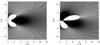 |
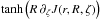
Fig. A.1
Contour plots of tanh(J(r,R,ζ)) and
|
| Open with DEXTER | |
Differentiation and taking limits can be interchanged with the integration only under particular conditions imposed on the function under the integration sign. If not said otherwise, we assume that these conditions are met. For this reason, the case of an infinitesimally thin disk (with f(z) = δ(z)) must be treated separately.
The expression for R∂RΨ(R,Z)
in Sect. 2 involves an integral
 The
integral can be written as a sum
The
integral can be written as a sum 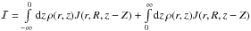 if the two summands exist.
By substituting
if the two summands exist.
By substituting  ,
the first integral can be rewritten as
,
the first integral can be rewritten as 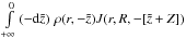 , and next, since
ρ(r, −
ζ) = ρ(r,ζ) and
J(r,R, −
ζ) = J(r,R,ζ),
as
, and next, since
ρ(r, −
ζ) = ρ(r,ζ) and
J(r,R, −
ζ) = J(r,R,ζ),
as 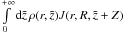 .
Finally, by renaming
.
Finally, by renaming  , we obtain
This proves Eq. (2).
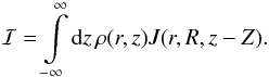
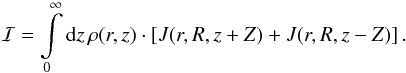
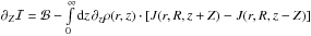
The integral expression for the vertical gradient of rotation in the quasi-circular
orbit approximation can be proved by performing a partial differentiation of
ℐ under the integration
sign: 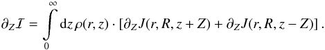 Now,
∂ZJ(r,R,z
± Z) = ±
∂zJ(r,R,z
± Z), which implies that
Now,
∂ZJ(r,R,z
± Z) = ±
∂zJ(r,R,z
± Z), which implies that
 .
Integration by parts under usual conditions gives
.
Integration by parts under usual conditions gives
 ,
where ℬ = (limz → +
∞ρ(r,z)[J(r,R,z
+ Z) − J(r,R,z −
Z)]) −
(ρ(r,0+)[J(r,R,Z)
− J(r,R, − Z)]) is
a boundary term. The expression in the first round bracket in this term is zero for any
finite Z,R,r, on account of the vanishing of the
difference in the square bracket and the vanishing of ρ in the same limit (it
suffices to assume a finite support of ρ). The expression in the second round bracket
also vanishes for finite ρ(r,0) since J is an even function of
the third argument. Hence, the boundary term ℬ also vanishes. Formally, one should also verify whether the
integration with respect to r and taking the above limit z → + ∞ commute, as there
is an integration over r present in the expression for R∂RΨ.
When this requirement is met, we have
,
where ℬ = (limz → +
∞ρ(r,z)[J(r,R,z
+ Z) − J(r,R,z −
Z)]) −
(ρ(r,0+)[J(r,R,Z)
− J(r,R, − Z)]) is
a boundary term. The expression in the first round bracket in this term is zero for any
finite Z,R,r, on account of the vanishing of the
difference in the square bracket and the vanishing of ρ in the same limit (it
suffices to assume a finite support of ρ). The expression in the second round bracket
also vanishes for finite ρ(r,0) since J is an even function of
the third argument. Hence, the boundary term ℬ also vanishes. Formally, one should also verify whether the
integration with respect to r and taking the above limit z → + ∞ commute, as there
is an integration over r present in the expression for R∂RΨ.
When this requirement is met, we have 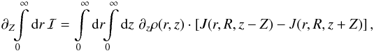 which
proves Eq. (3).
which
proves Eq. (3).
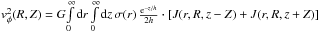
A.2. A special case: the exponential vertical profile
In the case of the vertical exponential falloff of the density profile,
 , the calculation of the
integrals in Eqs. (2) and (3) can be simplified. Then,
, the calculation of the
integrals in Eqs. (2) and (3) can be simplified. Then,
 and
and
 .
Now, both vφ(R,Z)
and ∂Zvφ(R,Z)
can be expressed in terms of two integrals I+ and I−:
.
Now, both vφ(R,Z)
and ∂Zvφ(R,Z)
can be expressed in terms of two integrals I+ and I−:
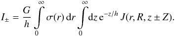 Namely,
for ,
Namely,
for ,
 and
and 
A.3. Qualitative properties of the vertical gradient of rotation and the presence of turn-overs
Equation (3) involves an integral
 [ J(r,R,z −
Z)−
J(r,R,z + Z) ]
that equals
[ J(r,R,z −
Z)−
J(r,R,z + Z) ]
that equals  J(r,R,Z −
z), owing to the symmetry of J and f. Now, consider
| Z |
>A>
0 large enough, beyond the main mass concentration, such that
J(r,R,Z −
z), owing to the symmetry of J and f. Now, consider
| Z |
>A>
0 large enough, beyond the main mass concentration, such that
 (by
assumption
(by
assumption  ). For
such Z,
only a region | z | ≪ |
Z | contributes to
). For
such Z,
only a region | z | ≪ |
Z | contributes to
 ,
and we can use the approximation formula J(r,R,Z − z) −
J(r,R,Z) ≈ −z∂ZJ(r,R,Z)
to obtain
,
and we can use the approximation formula J(r,R,Z − z) −
J(r,R,Z) ≈ −z∂ZJ(r,R,Z)
to obtain  .
Since f(z) and zf(z)
vanish at the infinity, integrating by parts gives
.
Since f(z) and zf(z)
vanish at the infinity, integrating by parts gives
 . On the other hand, for
f(z) =
δ(z) and for Z ≠ 0,
. On the other hand, for
f(z) =
δ(z) and for Z ≠ 0,
 . Hence, we obtain an
intuitively clear result: for all finite-width thin disks with the same column mass
density σ(r), the behavior of the vertical
gradient at high enough altitudes is universal and the same as for an infinitesimally
thin disk with surface mass density σ(r).
. Hence, we obtain an
intuitively clear result: for all finite-width thin disks with the same column mass
density σ(r), the behavior of the vertical
gradient at high enough altitudes is universal and the same as for an infinitesimally
thin disk with surface mass density σ(r).
Another qualitative result is obtained in the limit Z → 0. For
Z ≠ 0,
 ,
thus
,
thus  by continuity of
as a function of Z, and the vertical gradient is zero at
Z = 0, at
least for the mass distributions for which the usual theorems on the continuity of
functions defined by integrals Eq. (3)
apply.
by continuity of
as a function of Z, and the vertical gradient is zero at
Z = 0, at
least for the mass distributions for which the usual theorems on the continuity of
functions defined by integrals Eq. (3)
apply.
However, there is an exception from the above continuity behavior of the gradient lines
at Z = 0.
It is important to remember that the operation of taking various limits and the
operation of integration are not interchangeable in general. In particular, an integral
of a function sequence consisting of continuous functions with a parameter can result in
a discontinuous function of that parameter. For f(z) =
δn(z),
where δn is a functional
sequence representing the Dirac δ, the result of continuity of the gradient does
not necessarily follow and we can have a nonzero value in the same limit, in which case
the integral Eq. (3) is discontinuous at
Z = 0. To
give a simple example of what then may happen, consider a function sequence
 ,
then
,
then  , with
 .
Now, consider a limiting function g(x) = limn → +
∞gn(x)
and see if it is continuous at x = 0. For x = 0, g(0) ≡ limn → +
∞gn(0) = 0, whereas
for x ≠ 0,
.
Now, consider a limiting function g(x) = limn → +
∞gn(x)
and see if it is continuous at x = 0. For x = 0, g(0) ≡ limn → +
∞gn(0) = 0, whereas
for x ≠ 0,
 ,
thus, g(0) = 0 ≠ 1 =
limx → 0g(x),
therefore g(x) is discontinuous at
x = 0.
Now, think of the gradient lines in Fig. 7 – then
the finite disk corresponds to the situation described by gn(x)
(h =
n-1 > 0),
whereas the infinitesimally thin disk corresponds to the situation of discontinuous
g(x) (h = 0).
,
thus, g(0) = 0 ≠ 1 =
limx → 0g(x),
therefore g(x) is discontinuous at
x = 0.
Now, think of the gradient lines in Fig. 7 – then
the finite disk corresponds to the situation described by gn(x)
(h =
n-1 > 0),
whereas the infinitesimally thin disk corresponds to the situation of discontinuous
g(x) (h = 0).
Finally, we may try to understand the occurrence of the turn-overs in the gradient lines for h > 0, such as those seen in Fig. 10 or Fig. 7. First, note that a gradient line must asymptotically converge to zero, which is the universal asymptotics property discussed earlier. Second, the gradient line starts from 0 at Z = 0, which we have also seen above. Now, we perform a mapping of the region 0 < Z < +∞ to an interval 0 < Z < 1 by means of a transformation Z → tanhZ. Then the transformed gradient lines are continuous for 0 ≤ Z ≤ 1 and vanish at the boundaries. Next, we apply the Rolle theorem on continuously differentiable functions that vanish on the boundaries of a compact and simply connected interval, and we infer that there must be at least one point inside the interval where the gradient line has a local minimum, which explains the presence of a turn-over. The Rolle theorem does not apply to gradient lines of the infinitesimally thin disk, because of the discontinuity, and the analogous turn-overs do not have to occur, which is the case in Figs. 7 or 10.
© ESO, 2014
Current usage metrics show cumulative count of Article Views (full-text article views including HTML views, PDF and ePub downloads, according to the available data) and Abstracts Views on Vision4Press platform.
Data correspond to usage on the plateform after 2015. The current usage metrics is available 48-96 hours after online publication and is updated daily on week days.
Initial download of the metrics may take a while.