| Issue |
A&A
Volume 566, June 2014
|
|
|---|---|---|
| Article Number | A42 | |
| Number of page(s) | 9 | |
| Section | Cosmology (including clusters of galaxies) | |
| DOI | https://doi.org/10.1051/0004-6361/201321605 | |
| Published online | 05 June 2014 | |
Multifrequency constraints on the nonthermal pressure in galaxy clusters
1 INAF – Osservatorio Astronomico di Roma via Frascati 33, 00040 Monteporzio, Italy
e-mail: This email address is being protected from spambots. You need JavaScript enabled to view it.
, This email address is being protected from spambots. You need JavaScript enabled to view it.
2 School of Physics, University of the Witwatersrand, Johannesburg Wits 2050, South Africa
Received: 30 March 2013
Accepted: 25 November 2013
Abstract
Context. The origin of radio halos in galaxy clusters is still unknown and is the subject of a vibrant debate from both observational and theoretical points of view. In particular, the amount and the nature of nonthermal plasma and of the magnetic field energy density in clusters hosting radio halos is still unclear.
Aims. The aim of this paper is to derive an estimate of the pressure ratio X = Pnon − th/Pth between the nonthermal and thermal plasma in radio halo clusters that have combined radio, X-ray and Sunyaev-Zel’dovich (SZ) effect observations.
Methods. From the simultaneous P1.4 − LX and P1,4 − YSZ correlations for a sample of clusters observed with Planck, we derive a correlation between YSZ and LX that we use to derive a value for X. This is possible since the Compton parameter YSZ is proportional to the total plasma pressure in the cluster, which we characterize as the sum of the thermal and nonthermal pressure, while the X-ray luminosity LX is proportional only to the thermal pressure of the intracluster plasma.
Results. Our results indicate that the average (best-fit) value of the pressure ratio in a self-similar cluster formation model is X = 0.55 ± 0.05 in the case of an isothermal β-model with β = 2/3 and a core radius rc = 0.3·R500, holding on average for the cluster sample. We also show that the theoretical prediction for the YSZ − LX correlation in this model has a slope that is steeper than the best-fit value for the available data. The agreement with the data can be recovered if the pressure ratio X decreases with increasing X-ray luminosity as LX-0.96.
Conclusions. We conclude that the available data on radio halo clusters indicate a substantial amount of nonthermal pressure in cluster atmospheres whose value must decrease with increasing X-ray luminosity or increasing cluster mass (temperature). This is in agreement with the idea that nonthermal pressure is related to nonthermal sources of cosmic rays that live in cluster cores and inject nonthermal plasma in the cluster atmospheres, which is subsequently diluted by the intracluster medium acquired during cluster collapse, and has relevant impact for further studies of high-energy phenomena in galaxy clusters.
Key words: galaxies: clusters: general / cosmic background radiation / galaxies: clusters: intracluster medium / cosmology: theory
© ESO, 2014
1. Introduction
The origin of radio halos (RHs) in galaxy clusters is a long-standing, but still open problem. Various scenarios have been proposed that refer to primary electron models (see, e.g., Sarazin 1999; Miniati et al. 2001), reacceleration models (see, e.g., Brunetti et al. 2009), secondary electron models (see, e.g., Blasi & Colafrancesco 1999; Miniati et al. 2001; Pfrommer et al. 2008), and also geometrical projection effect models (see, e.g., Skillman et al. 2013). Each one of these models has both interesting and contradictory aspects, but each one relies on the presence of a population of relativistic electrons (and positrons) and of a large-scale magnetic field that are spatially distributed in the cluster atmosphere. In the following, we assume that RHs are produced by an intrinsic relativistic electron population within the cluster atmosphere. The presence of RHs in clusters requires an additional nonthermal pressure (energy density) component in addition to the thermal pressure (energy density) provided by the intracluster medium (ICM).
It has been recognized that galaxy clusters hosting RHs show a correlation between their radio power measured at 1.4 GHz P1.4 due to synchrotron emission, and their X-ray luminosity LX due to thermal bremsstrahlung emission (see, e.g., Colafrancesco 1999; Giovannini et al. 2000; Feretti et al. 2012) that can be fitted with a power law  with slope d lying in the range 1.5 to 2.1 (see, e.g., Brunetti et al. 2009, for a recent compilation). Such a correlation links the nonthermal particle and magnetic field energy density (pressure) related to the synchrotron radio luminosity
  (where α is the slope of a power-law electron spectrum ne,rel ~ E− α), with the thermal pressure Pth of the ICM, related to the thermal bremsstrahlung X-ray emission given by
  , where Pth ∝ neT and
  .
.
An analogous correlation has been found (see, e.g., Basu 2012) between P1.4 and the integrated Compton parameter YSZ due to the Suyaev-Zel’dovich effect (SZE) produced by Inverse Compton Scattering of CMB photons off the electron populations which are residing in the cluster atmosphere (see Colafrancesco et al. 2003, for details; and Colafrancesco 2012, for a recent review). The Compton parameter YSZ ∝ ∫dℓPtot is proportional to the total particle pressure (energy density) provided by all the electron populations in the clusters atmosphere (see Colafrancesco et al. 2003): the cluster atmosphere is thus the combination of the thermal plasma producing X-ray emission and the nonthermal plasma, at least the one producing synchrotron radio emission. Therefore, the P1.4 − YSZ correlation links the nonthermal particle and B-field pressures, as measured by P1.4, with the total particle pressure Ptot, as measured by YSZ. For the sake of generality here we express the total particle pressure Ptot as ![Mathematical equation: \begin{equation} P_{\rm tot} = P_{\rm th} + P_{\rm non-th} = P_{\rm th} \bigg[1 + X \bigg] \label{eq.X} \end{equation}](/articles/aa/full_html/2014/06/aa21605-13/aa21605-13-eq28.png) (1)where X ≡ Pnon − th/Pth.
(1)where X ≡ Pnon − th/Pth.
The correlated X-ray, SZE, and radio emission from RH clusters, as shown by the P1.4 − LX and P1.4 − YSZ relations, indicate that the RH cluster atmospheres must also exhibit a relation between the thermal ICM pressure Pth and the nonthermal particle pressure Pnon − th, which can be hence constrained by observations.
In this paper, we will discuss the constraints on the quantity X set by the available radio, X-ray, and SZE information on a sample of RH clusters observed by Planck. In Sect. 2, we discuss the cluster data that we use in our analysis, and in Sect. 3 we discuss the theoretical approach to deriving information on the pressure ratio X. We discuss our results and draw our conclusions in Sect. 4.
We assume throughout the paper a flat, vacuum-dominated Universe with Ωm = 0.32 and ΩΛ = 0.68 and H0 = 67.3 km s-1 Mpc-1.
2. The cluster sample
We consider here a sample of galaxy clusters that exhibit RHs and that also have X-ray and SZE information. The cluster data that are used in our analysis are selected from the Planck Collaboration VIII (2011) and from Brunetti et al. (2009). The cluster redshifts and the radio power P1.4 are taken from Brunetti et al. (2009) and from Giovannini et al. (2009), the bolometric X-ray luminosity LX are taken from Reichert et al. (2011), while the integrated Compton parameter YSZ are taken from the Planck Collaboration VIII (2011). We also used information on the cluster velocity dispersion collected from various authors like Wu et al. (1999), Zhang et al. (2011). As for the cluster A781, we used the information given by Cook et al. (2012) and from Geller et al. (2013) Our final cluster sample extends the cluster sample considered by Basu (2012) by including some additional clusters for which the integrated Compton parameter is now available. The final RH cluster sample we use in this work is reported in Tables 1 and 2. Table 1 reports the values of the cluster radio halo power P1.4, the bolometric X-ray luminosity LX and the redshift z. Table 2 reports, for the same clusters in Table 1, the values of the integrated Compton parameter YSZ. Since the values of the cosmological parameters have been updated to the new values given by the Planck Collaboration XXIX (2013), we rescale the LX and P1.4 values in order to accommodate them to the new cosmological model used here. We rescale our P1.4 as follows:  (2)and for the bolometric luminosity LX, we obtain
  (3)where the dashes represent the new value. As for the Compton parameter, we simply re-calculated
  using the new cosmological values.
RH clusters sample.
2.1. Correlations
The sample of RH clusters we consider in this paper exhibits the P1.4 − LX and P1.4 − YSZ correlations shown in Figs. 1 and 2. Because of the common variable P1.4 in both correlations shown in Figs. 1 and 2, a correlation between YSZ and LX is then expected theoretically and it is actually found in the data (see Fig. 3).
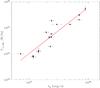 |
Fig. 1 Best-fit power-law relation |

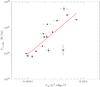 |
Fig. 2 Best-fit power-law relation |

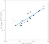 |
Fig. 3 Correlation between Ysph,R500·E9/4(z) and LX correlation for the cluster sample we consider in this paper. The best-fit power-law relation has a slope m = 0.89 ± 0.05 and a normalization of log c = −44.11 ± 2.23 and it is represented by the solid blue curve. The dashed curves showing the uncertainties in the slope of the correlation are shown in cyan. |
To fit the P1.4–LX, the P1.4–YSZ and the YSZ–Lx correlations, we have adopted the approach of Akritas & Berchady (1996). According to this approach, to fit a straight line y = mx + c to a data set, the slope and the intercept are given as follows: 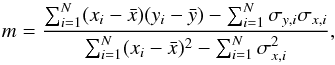 (4)and
  (5)where
  is the mean of x and same for y. The quantities σx,i and σy,i are the errors in x and y. A proper treatment of the error propagation shows that the variance in the slope and in the normalization of the best-fit line can be computed as
 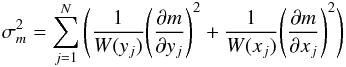 (6)
(6)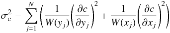 (7)where
  (8)and
  (9)In addition to the previous analysis of the variance in the slope and of the normalization, a further treatment is needed here to take the intrinsic scatter in the data into account. To estimate this intrinsic scatter, we follow the method outlined in Akritas & Berchady (1996), which we summarize as follows:
  (10)where Ri is the residual. Then the intrinsic scatter
  is estimated as follows
  (11)The χ2 is then written as
  (12)where
  and
and  are the corresponding variances of xi and yi, respectively.
Our analysis yields the correlations  with best-fit parameters log C = −56.04 ± 3.18 and d = 1.78 ± 0.07, and
  with best-fit parameters log B = 31.16 ± 0.36 and a = 1.80 ± 0.10. The results obtained here are quite consistent with those obtained by Brunetti et al. (2009), where d was found to be in the range of 1.5 ÷ 2.1 and log C in the range −55.4 ÷ − 60.85, and with the analysis of Basu (2012), who obtained log B = 32.1 ± 1 and a = 2.03 ± 0.28 for the Brunetti et al. (2009) RH sample.
The same data also exhibit a correlation between the Compton parameter  and the X-ray bolometric luminosity LX. Our analysis of this power-law correlation
  provides a best-fit slope of m = 0.89 ± 0.05 and a normalization of log c = −44.11 ± 2.23.
3. Theoretical analysis
The characteristic quantities that describe the galaxy cluster structure are defined in a simple self-similar model (see, e.g., Arnaud et al. 2010, and references therein). First, we derive a relation between the Compton parameter Ysph,500 and the bolometric X-ray luminosity LX for a general cluster in the case of a constant ICM density over R500. Then, following the same approach, we derive the same relation for the more realistic case of an isothermal β-model for the radial profile of the ICM number density. The final results presented in this paper refer to the case of the isothermal β-model.
The mass M500 is defined as the mass within the radius R500 at which the mean mass density of the cluster is 500 times the critical density, ρc(z), of the Universe at the cluster redshift  (13)with ρc(z) = 3H2(z)/(8πG). Here H(z) is the Hubble constant given by H(z) = H(0) [ΩM = (1 + z)3 + ΩΛ] 1/2 and G is the Newtonian constant of gravitation.
The characteristic thermal pressure of the cluster ICM at R500 is defined as  (14)where ne,500 and kT500 are the thermal ICM electron numbers density and temperature, respectively. The electron number density is defined as
  (15)(see Arnaud et al. 2010), where ρg,500 = 500fBρc(z) with fB = 0.175 being the baryonic-fraction of the Universe, mp is the proton mass, and μe ≈ 1.14 is the mean molecular weight of the gas per free electron. The temperature T500 can be expressed as
  (16)where μ is the mean molecular weight. The temperature T500 is hence the uniform temperature of an isothermal sphere with mass M500 and radius R500.
The characteristic bremsstrahlung X-ray luminosity (see, e.g. Rybicki & Lightman 1985) of a cluster can be written as  (17)where
  . The normalization constant C2 in the previous Eq. (17) takes the value of 1.728 × 10-40 W s-1 K−½ m3.
The characteristic integrated spherical Compton parameter calculated within the radius R500 can be written as  (18)We have previously denoted with
  the cylindrical Compton parameter within a radius 5·R500 and here we introduce as Ysph,R500 the spherical Compton parameter within the radius R500. We note that the spherical Compton parameter is equal to the cylindrical Compton parameter within the radius 5·R500 as pointed out by Arnaud et al. (2010). Since the Integrated Compton parameter given for the SZE data by the Planck Collaboration VIII (2011) is measured at a radius of 5·R500, we scale the data of the Compton parameter given by the Planck Collaboration VIII (2011) down to R500 using the relation given in Arnaud et al. (2010) as follows:
  (19)where the value of I(1) = 0.6552 and I(5) = 1.1885. These values are given in the Appendix of Arnaud et al. (2010).
3.1. The YSZ–LX relation
We derive here the correlation between the spherical integrated Compton parameter Ysph,R500 and the bremsstrahlung bolometric X-ray Luminosity LX by using the simple self-similar cluster model previously discussed. The correlation between the spherical Compton parameter Ysph,R500 and the bolometric X-ray luminosity LX shown by our cluster sample is given in Fig. 3. We derive the theoretical relation between the integrated Compton parameter and the bolometric X-ray luminosity by using Eqs. (17), (18) first assuming a distribution of the plasma with a constant density over R500, and then we generalize the same relation to a more realistic density distribution. The slope of the correlation is, in fact, independent of the assumed cluster density profile while it affects only its normalization. Combining Eqs. (13)−(18) and eliminating R500, we obtain ![Mathematical equation: \begin{eqnarray} Y_{{\rm sph},R500} E^\frac{9}{4}(z)&= & \displaystyle{\frac{\displaystyle{\Bigg(1+X \Bigg) \frac{8 \pi^2}{9}}\displaystyle{\Bigg(\frac{\sigma_{\rm T} G m_{\rm p} \mu 500 \rho_{\rm c} n_{\rm e}}{m_{\rm e} c^2}\Bigg)}}{\Bigg[\displaystyle{\frac{4 \pi}{3}C_2 n_{\rm e}^2}\displaystyle{\Bigg(\frac{2}{3 k_{\rm B}} \pi G \mu 500 \rho_{\rm c} m_{\rm p} \Bigg)^\frac{1}{2}}\Bigg]^\frac{5}{4}}} \nonumber \\ && \times\, \displaystyle{\Bigg(\frac{L_{\rm X}}{10^7~\rm erg/s}\Bigg)^\frac{5}{4}} \cdot \label{eq.ysz_lx_nconst} \end{eqnarray}](/articles/aa/full_html/2014/06/aa21605-13/aa21605-13-eq176.png) (20)The quantity E(z) is the ratio of the Hubble constant at redshift z to its present value, H0, i.e., E(z) = [ΩM(1 + z)3 + ΩΛ] 1/2. To estimate the best-fit value of X from our cluster sample we minimize the χ2 for the YSZ − LX relation with respect to the value X. First, we consider the case in which the pressure ratio X is constant and therefore, the nonthermal pressure has the same radial distribution of the thermal plasma in the cluster. We will discuss the impact of this assumption on our results in Sect. 4.
(20)The quantity E(z) is the ratio of the Hubble constant at redshift z to its present value, H0, i.e., E(z) = [ΩM(1 + z)3 + ΩΛ] 1/2. To estimate the best-fit value of X from our cluster sample we minimize the χ2 for the YSZ − LX relation with respect to the value X. First, we consider the case in which the pressure ratio X is constant and therefore, the nonthermal pressure has the same radial distribution of the thermal plasma in the cluster. We will discuss the impact of this assumption on our results in Sect. 4.
We now compute the same correlation Ysph,R500 − LX by using a more realistic, but still simple, isothermal β-model (see, e.g., Sarazin 1988, for a review) in which the ICM is assumed to be in hydrostatic equilibrium with the pressure balancing gravity. Following Ota & Mitsuda (2004), the equation for hydrostatic equilibrium is written as  (21)where M(r) is the total mass enclosed in a radius r. In a simple β-model density profile
 ![Mathematical equation: \hbox{$ \rho_{\rm g}(r)=\rho_{\rm g,0} \bigg[1+ \bigg(\frac{r}{r_{\rm c}}\bigg)^2 \bigg]^{-\frac{3\beta}{2}}$}](/articles/aa/full_html/2014/06/aa21605-13/aa21605-13-eq185.png) where ρg,0 is the central gas density, rc the core radius and β has usually values ~0.5 ÷ 1, and the mean total density
where ρg,0 is the central gas density, rc the core radius and β has usually values ~0.5 ÷ 1, and the mean total density  inside a radius of r is given by
  (22)where
  is the central total density of the cluster. From this we write the central gas number density as
  (23)Then, using Eqs. (17) and (18) and writing rc = λR500, we cast the central gas number density as
  (24)Several values of λ have been used by different authors (see, e.g., Bahcall 1975; Sarazin 1988; Dressler 1978) suggesting that for typical rich clusters the value of λ is in the range 0.1 ÷ 0.25. For X-ray clusters the value of λ can even go up to 0.3. Here we adopt the value of λ = 0.3, which yields consistent values of X ≥ 0 for the majority of the RH clusters in our sample. We notice, in fact, that the value of X is sensitive to the central number density in the formalism we adopt here, with large values of the central density leading to large values of X. We stress that this description assumes that the nonthermal plasma is distributed spatially as the thermal ICM, and that the pressure ratio X is therefore spatially constant. Relaxing this assumption can provide slightly different results, which we will discuss in a further analysis of the radial distribution of the cluster pressure structure (Colafrancesco et al., in prep.).
Under the β-model density profile assumption, the spherical integrated Compton parameter and the X-ray luminosity within R500 can be written as  (25)and
  (26)where
  (27)and
  (28)In order to clarify the main dependence of the integrated Compton parameter from the bolometric X-ray luminosity, we condense Eqs. (25), (26) into a compact form similar to Eq. (20)
 ![Mathematical equation: \begin{equation} Y_{{\rm sph},R500} E(z)^{9/4} = \bigg[{(1+X) Y_0 \over L^{5/4}_0}\bigg] L_{\rm X}^{5/4} , \end{equation}](/articles/aa/full_html/2014/06/aa21605-13/aa21605-13-eq205.png) (29)where we have defined the following quantities
(29)where we have defined the following quantities  (30)and
  (31)The theoretical prediction for a constant value of X for all clusters is shown in Fig. 4 together with the best-fit correlation of the data. We stress that the theoretical curve calculated under these assumptions is sensitively steeper than the power-law best-fit to the data. This is the result of having assumed a constant value of X for all cluster X-ray luminosities in our model. A decreasing value of X with the X-ray luminosity (or with the Compton parameter) as
  can alleviate the problem, providing a better agreement between the cluster formation scenario and the nonthermal phenomena in RH clusters.
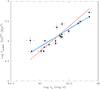 |
Fig. 4 Best-fit line (solid blue) together with the associated uncertainties in the slope and intercept (dashed cyan) and the theoretical expectation (solid red) for the Ysph,R500 − LX relation. The best-fit value of X is 0.55 ± 0.05 for the case of an isothermal β-model with a core radius of rc = 0.3R500 and β = 2/3. |
To analyze this point, we compute the value of X for each individual cluster in our sample by using the relationship between the Compton parameter and the X-ray bolometric luminosity given above. Table 3 reports the values of X calculated for the considered clusters assuming the previous β-model. The error in X is calculated from the error in the luminosity and the Compton parameter. It is given by  (32)It is interesting that the analysis presented in this paper can provide a barometric test of the overall pressure structure in galaxy clusters that can also be useful for future studies.
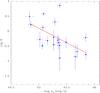 |
Fig. 5 Behavior of the pressure ratio X as a function of the cluster X-ray bolometric luminosity for the cluster sample. The best fit curve |
Clusters name and their corresponding calculated X parameters.
Figure 5 shows the correlation of the values of X with both the Compton parameter and with the bolometric X-ray luminosity of each cluster. The data and our estimate for X show that there is a clear decreasing trend of the pressure ratio X with both the cluster X-ray luminosity and with the integrated Compton parameter indicating that low-LX (mass) cluster hosting RHs require a larger ratio of the nonthermal to thermal pressure ratio. We fit the X − LX relation in Fig. 5 by assuming a power-law form  (33)and we obtain best-fit values of ξ = 0.96 ± 0.16 and log Q = 43.49 ± 7.09. The best-fit curve with these parameters is also shown in Fig. 5. A
  (with 17 d.o.f.) is obtained in the case of
  , while a value
  (with 18 d.o.f.) is obtained in the case X = const. This shows that the behavior is statistically significative: in fact, the probability of having a
  that is larger than 1.14 (1.56) with 17 (18) d.o.f. is 0.307 (0.061). The best-fit value of the exponent ξ = 0.96 is different from 0 at the 6 sigma confidence level.
For the sake of completeness, we also show in Fig. 6 the correlation between the total pressure ratio 1 + X and LX that is fitted with a power-law of the form  with best-fit values ξ′ = 0.38 ± 0.05 and log Q′ = 17.50 ± 2.49. Analogously, we find that a
  (with 17 d.o.f.) is obtained in the case of
  , while a value
  (with 18 d.o.f.) is obtained in the case (1 + X) =const. Also, in this case, we find that the decrease of 1 + X with the cluster X-ray luminosity is statistically significant: the probability of having a that is larger than 1.00 (1.33) with 17 (18) d.o.f. is 0.454 (0.157).
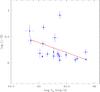 |
Fig. 6 Behavior of the total pressure ratio 1 + X as a function of the cluster X-ray bolometric luminosity for the cluster sample. The best-fit curve |

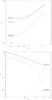 |
Fig. 7 Behavior of the pressure ratio X as a function of the cluster β parameter (upper panel) and as a function of the parameter λ (lower panel) for some of the RH clusters in our list. |
We then calculate our theoretical prediction for the Ysph,R500 − LX relation, using the previous  relation and indeed we find a better agreement of the cluster formation model with the available data for our sample of RH clusters (see Fig. 8). This is confirmed by the reduced χ2 analysis. We have calculated the values of the
  in two cases: a constant value of X and the case in which we insert the relation
  , as it results from our analysis of the extended sample of clusters we consider after the Planck SZ catalog release. The for the case with a varying X, i.e., using the best fit
  , is 0.96 (with 17 d.o.f.), while it is 0.86 (with 18 d.o.f.) in the case in which X = const. This indicates that the fit to the data with a value of X decreasing with the cluster X-ray luminosity is able to reproduce the correlation of the data better than in the case X = const., thus bringing consistency and robustness to our analysis and results.
Our result indicates that the existence of a nonthermal pressure in RH clusters with the ratio X = Pnon − th/Pth which decreases with cluster X-ray luminosity (or mass) is able to recover the consistency between the theoretical model for cluster formation and the presence of RHs in clusters.
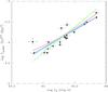 |
Fig. 8 Best-fit line to the data (solid blue) together with the associated uncertainties in the slope and intercept (dashed cyan) and the theoretical expectation (solid red curve). The relation |
Figure 9 shows the theoretical prediction for the Ysph,R500 − LX relation using the best-fit correlation between the total pressure ratio and the bolometric X-ray luminosity,  .
.
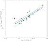 |
Fig. 9 Best-fit line to the data (solid blue) together with the associated uncertainties in the slope and intercept (dashed cyan) and the theoretical expectation (solid red curve). The relation |

Here, the for the case in which we insert the relation  is 0.97 (with 17 d.o.f.), while it is 0.86 (with 18 d.o.f.) in the case in which 1 + X = const. This again shows that the fit to the data with a value of 1 + X decreasing with the cluster X-ray luminosity is better than in the case 1 + X = const., and it is consistent with the best-fit analysis of the (1 + X) − LX correlation.
4. Discussion and conclusions
We found evidence that the largest available sample of RH clusters with combined radio, X-ray and SZE data require substantial nonthermal particle pressure to sustain their diffuse radio emission and to be consistent with the SZE and X-ray data. This result has been derived mainly from the Ysph,R500 − LX relation for a sample of RH clusters selected from the Planck SZ effect survey. This nonthermal particle (electron and positron) pressure affects the value of the total Compton parameter Ysph,R500 within R500 in particular, indicating an integrated Compton parameter that is a factor ~0.55 ± 0.05 (on average) larger that the one induced by the thermal ICM alone.
The shape of the Ysph,R500 − LX does not depend on the assumptions of the cluster parameters and density profiles, while its normalization (and therefore the value of X) depends on the cluster parameters. Specifically, the value of X decreases with increasing cluster core radius (or increasing value of λ) and increases with increasing value of the central particle density (see Fig. 7). Therefore, the normalization of the previous correlation, and consequently the best-fit value of X, are affected by the cluster structural parameters. Detailed studies of the values of X derived from the previous correlation could then be used as barometric probes of the structure of cluster atmospheres. However, one of the most important results we obtained in this work is that the simple description in which X is constant for every cluster fails to reproduce the observed Ysph,R500 − LX relation, requiring that  . We hence found that the impact of the nonthermal particle pressure is larger (in a relative sense) in low-LX RH clusters than in high-LX RH clusters, requiring a luminosity evolution of the pressure ratio with ξ ≈ 0.96 ± 0.16. In fact, without this luminosity evolution, the theoretical model for the YsphR500 − LX correlation predicts a steeper relation compared to the best-fit correlation which is considerably flatter. A decreasing value of X with the X-ray luminosity can, therefore, provide a better agreement between the cluster formation scenario and the presence of nonthermal phenomena in RH clusters. This behavior can be attributed to the decreasing impact of the nongravitational processes in clusters going from low to high values of LX. This is consistent with a scenario in which relativistic electrons and protons are injected at an early cluster age by one or more cosmic ray sources and then diffuse and accumulate in the cluster atmosphere, but are eventually diluted by the infalling (accreting) thermal plasma. This fact is also consistent with the outcomes of relativistic covariant kinetic theories of shock acceleration in galaxy clusters (see, e.g., Wolfe & Melia 2006, 2008) which predict that the major effect of shocks and mergers is to heat the ICM (rather than accelerating electrons at relativistic energies): in such a case, the relative contribution of nonthermal particles to the total pressure in clusters should decrease with increasing cluster temperature, or X-ray luminosity since these two quantities are strongly correlated. Detailed models of the origin and distribution of the Pnon − th could challenge the results presented here and we will discuss the relative phenomenology elsewhere (Colafrancesco et al., in prep.).
The positive values of X found in our cluster analysis indicates the presence of a considerable nonthermal pressure provided by nonthermal electrons (and positrons): the presence of nonthermal electrons (positrons) is the minimal particle energy density requirement because it has been derived from SZE measurements (i.e., by Compton scattering of CMB photons off high-energy electrons, and positrons). For a complete understanding of the overall cluster pressure structure one should also consider the additional contribution of nonthermal proton, which is higher than the electron one since protons lose energy on a much longer timescale. Therefore, the derived values of X should be considered as lower limits on the actual total nonthermal pressure and this will point to the presence of a relatively light nonthermal plasma in cluster atmospheres. A full understanding of the proton energy density (pressure) in cluster atmospheres could be obtained by future gamma-ray observations (or limits) of these galaxy clusters with RHs because the gamma-ray emission could possibly be produced by π0 → γ + γ decays where the neutral pions π0 are the messengers of the presence of hadrons (protons) in cluster atmospheres (see, e.g., Colafrancesco & Blasi 1998; Marchegiani et al. 2007; Colafrancesco & Marchegiani 2008, and references therein). We will address the consequences of this issue of the high-E emission properties of RH clusters elsewhere (Colafrancesco et al., in prep.).
The results presented in this paper are quite independent of our assumptions of the cluster structural properties. Specifically, the slope of the Ysph,R500 − LX relation does not depend on the detailed shape of the cluster density profile, and hence the condition seems quite robust. However, the absolute value of the pressure ratio X for each cluster depends on the assumed density profile and on the simplifying assumption that the nonthermal electron distribution resembles the thermal ICM distribution. It might be considered, in general, that the nonthermal and thermal particle density radial distributions are correlated as ne,non − th(r) ∝ [ne,th(r)] α, and previous studies (see Colafrancesco & Marchegiani 2008) showed that the values of α do not strongly deviate from 1, thus rendering our assumption reasonable and our result robust.
In conclusion, we have shown that the combination of observations on RH clusters at different wavelengths (radio, mm., and X-rays) is able to provide physical constraints on the nonthermal particle content of galaxy clusters. This is possible by combining the relevant parameters carrying information on the nonthermal (i.e., the total Compton parameter) and thermal (i.e., the X-ray bremsstrahlung luminosity) pressure components residing in the cluster atmosphere. The next generation radio (e.g., the Square Kilometer Array and its precursors, like MeerKAT), mm. (e.g., Millimetron, and in general mm. experiment with spatially-resolved spectroscopic capabilities), and X-ray instruments will definitely shed light on the origin of radio halos in galaxy clusters and on their cosmological evolution.
Acknowledgments
S.C. acknowledges support by the South African Research Chairs Initiative of the Department of Science and Technology and National Research Foundation and by the Square Kilometre Array (SKA). M.S.E., P.M., and N.M. acknowledge support from the DST/NRF SKA post-graduate bursary initiative.
References
- Akritas, M., & Bershady, M. 1996, ApJ, 470, 706 [NASA ADS] [CrossRef] [Google Scholar]
- Arnaud, M., Pratt, G. W., Piffaretti, R., et al. 2010, A&A, 517, A92 [NASA ADS] [CrossRef] [EDP Sciences] [Google Scholar]
- Bahcall, N. A. 1975, ApJ, 198, 249 [NASA ADS] [CrossRef] [Google Scholar]
- Basu, K. 2012, MNRAS, 421, L112 [NASA ADS] [CrossRef] [Google Scholar]
- Blasi, P., & Colafrancesco, S. 1999, Astro Particle Physics, 12, 169 [NASA ADS] [CrossRef] [Google Scholar]
- Brunetti, G., Cassano, R., Dolag, K., & Setti, G. 2009, A&A, 507, 661 [NASA ADS] [CrossRef] [EDP Sciences] [Google Scholar]
- Colafrancesco, S. 1999, in Diffuse thermal and relativistic plasma in galaxy clusters, eds. H. Bohringer, L. Feretti, & P. Schuecker (Garching, Germany: Max-Planck-Institut fur Extraterrestrische Physik), 269 [Google Scholar]
- Colafrancesco, S. 2012, in Frontier objects between particle physics and astrophysics, Proc. Vulcano Workshop XIV (Italian Physical Society), in press [Google Scholar]
- Colafrancesco, S., & Blasi, P. 1998, Astropart. Phys., 9, 227 [NASA ADS] [CrossRef] [Google Scholar]
- Colafrancesco, S., & Marchegiani, P. 2008, A&A, 484, 51 [NASA ADS] [CrossRef] [EDP Sciences] [Google Scholar]
- Colafrancesco, S., Marchegiani, P., & Palladino, E. 2003, A&A, 397, 27 [NASA ADS] [CrossRef] [EDP Sciences] [Google Scholar]
- Cook, R., & Dell’Antonio, P. 2012, ApJ, 750, 14 [Google Scholar]
- Dressler, A. 1978, ApJ, 226, 55 [NASA ADS] [CrossRef] [Google Scholar]
- Enßlin, T., & Kaiser, C. 2000, A&A, 360, 417 [NASA ADS] [Google Scholar]
- Feretti, L., Giovannini, G., Govoni, F., & Murgia, M. 2012, A&ARv, 20, 54 [Google Scholar]
- Giovannini, G., & Feretti, L. 2000, New Astron., 5, 335 [NASA ADS] [CrossRef] [Google Scholar]
- Giovannini, G., Bonafede, A., Feretti, L., et al. 2009, A&A, 507, 1257 [NASA ADS] [CrossRef] [EDP Sciences] [Google Scholar]
- Kelly, B. C. 2007, ApJ, 665, 1489 [NASA ADS] [CrossRef] [Google Scholar]
- Marchegiani, P., Perola, G. C., & Colafrancesco, S. 2007, A&A, 465, 41 [NASA ADS] [CrossRef] [EDP Sciences] [Google Scholar]
- Miniati, F., Jones, T. W., Kang, H., & Ryu, D. 2001, ApJ, 562, 233 [NASA ADS] [CrossRef] [Google Scholar]
- Morandi, A., Ettori, S., & Moscardini, L. 2007, MNRAS, 379, 518 [NASA ADS] [CrossRef] [Google Scholar]
- Ota, N., & Mitsuda, K. 2004, A&A, 428, 754 [Google Scholar]
- Planck Collaboration VIII 2011, A&A, 536, A8 [NASA ADS] [CrossRef] [EDP Sciences] [Google Scholar]
- Planck Collaboration XXIX 2013, A&A, in press, DOI: 10.1051/0004-6361/201321523 [Google Scholar]
- Pfrommer, C., Enßlin, T. A., & Springel, V. 2008, MNRAS, 385, 1211 [NASA ADS] [CrossRef] [Google Scholar]
- Reed, B. C. 1992, Am. J. Phys., 60, 59 [NASA ADS] [CrossRef] [Google Scholar]
- Reichert, A., Böhringer, H., Fassbender, R., & Mühlegger, M. 2011, A&A, 535, A4 [NASA ADS] [CrossRef] [EDP Sciences] [Google Scholar]
- Rines, K., Geller, M. J., Diaferio, A., & Kurtz, M. J. 2013, ApJ, 767, 15 [Google Scholar]
- Rybicki, G. B., & Lightman, A. P. 1985, Radiative processes in astrophysics (New York: Wiley-VCH) [Google Scholar]
- Sarazin, C. L 1988, X-ray emission from clusters of galaxies (Cambridge: Cambridge Univ. Press) [Google Scholar]
- Sarazin, C. L. 1999, ApJ, 520, 529 [NASA ADS] [CrossRef] [Google Scholar]
- Skillman, S. W., Xu, H., Hallman, E. J., et al. 2013, ApJ, 765, 21 [NASA ADS] [CrossRef] [Google Scholar]
- Tremaine, S., Gebhardt, K., Bender, R., et al. 2002, ApJ, 574, 740 [NASA ADS] [CrossRef] [Google Scholar]
- Tucker, W., Blanco, P., Rappoport, S., et al. 1998, ApJ, 496, L5 [NASA ADS] [CrossRef] [Google Scholar]
- York, D. 1996, Can J. Phys., 44, 1079 [Google Scholar]
- Wolfe, B., & Melia, F. 2006, ApJ, 638, 125 [NASA ADS] [CrossRef] [Google Scholar]
- Wolfe, B., & Melia, F. 2008, ApJ, 675, 156 [NASA ADS] [CrossRef] [Google Scholar]
- Wu, F., Xue, Y., & Fang, L. 1999, ApJ, 524, 22 [NASA ADS] [CrossRef] [Google Scholar]
- Zhang, Y.-Y., Andernach, H., Caretta, C. A., et al. 2011, A&A, 526, A105 [NASA ADS] [CrossRef] [EDP Sciences] [Google Scholar]
All Tables
All Figures
|
Fig. 1 Best-fit power-law relation |
| In the text | |
|
Fig. 2 Best-fit power-law relation |
| In the text | |
|
Fig. 3 Correlation between Ysph,R500·E9/4(z) and LX correlation for the cluster sample we consider in this paper. The best-fit power-law relation has a slope m = 0.89 ± 0.05 and a normalization of log c = −44.11 ± 2.23 and it is represented by the solid blue curve. The dashed curves showing the uncertainties in the slope of the correlation are shown in cyan. |
| In the text | |
|
Fig. 4 Best-fit line (solid blue) together with the associated uncertainties in the slope and intercept (dashed cyan) and the theoretical expectation (solid red) for the Ysph,R500 − LX relation. The best-fit value of X is 0.55 ± 0.05 for the case of an isothermal β-model with a core radius of rc = 0.3R500 and β = 2/3. |
| In the text | |
|
Fig. 5 Behavior of the pressure ratio X as a function of the cluster X-ray bolometric luminosity for the cluster sample. The best fit curve |
| In the text | |
|
Fig. 6 Behavior of the total pressure ratio 1 + X as a function of the cluster X-ray bolometric luminosity for the cluster sample. The best-fit curve |
| In the text | |
|
Fig. 7 Behavior of the pressure ratio X as a function of the cluster β parameter (upper panel) and as a function of the parameter λ (lower panel) for some of the RH clusters in our list. |
| In the text | |
|
Fig. 8 Best-fit line to the data (solid blue) together with the associated uncertainties in the slope and intercept (dashed cyan) and the theoretical expectation (solid red curve). The relation |
| In the text | |
|
Fig. 9 Best-fit line to the data (solid blue) together with the associated uncertainties in the slope and intercept (dashed cyan) and the theoretical expectation (solid red curve). The relation |
| In the text | |
Current usage metrics show cumulative count of Article Views (full-text article views including HTML views, PDF and ePub downloads, according to the available data) and Abstracts Views on Vision4Press platform.
Data correspond to usage on the plateform after 2015. The current usage metrics is available 48-96 hours after online publication and is updated daily on week days.
Initial download of the metrics may take a while.