| Issue |
A&A
Volume 565, May 2014
|
|
|---|---|---|
| Article Number | A57 | |
| Number of page(s) | 7 | |
| Section | Stellar structure and evolution | |
| DOI | https://doi.org/10.1051/0004-6361/201423397 | |
| Published online | 08 May 2014 | |
The formation of long-period eccentric binaries with a helium white dwarf
Institut d’Astronomie et d’Astrophysique, Université Libre de
Bruxelles,
ULB, CP. 226, Boulevard du Triomphe,
1050
Brussels,
Belgium
e-mail:
This email address is being protected from spambots. You need JavaScript enabled to view it.
Received:
10
January
2014
Accepted:
18
March
2014
Abstract
The recent discovery of long-period eccentric binaries hosting a He-white dwarf or a subdwarf star has been challenging binary-star modeling. Based on accurate determinations of the stellar and orbital parameters for IP Eri, a K0 + He-WD system, we propose an evolutionary path that is able to explain the observational properties of this system and, in particular, to account for its high eccentricity (0.25). Our scenario invokes an enhanced-wind mass loss on the first red giant branch (RGB) in order to avoid mass transfer by Roche-lobe overflow, where tides systematically circularize the orbit. We explore how the evolution of the orbital parameters depends on the initial conditions and show that eccentricity can be preserved and even increased if the initial separation is large enough. The low spin velocity of the K0 giant implies that accretion of angular momentum from a (tidally-enhanced) RGB wind should not be efficient.
Key words: binaries: close / stars: evolution
© ESO, 2014
1. Introduction
The recent discovery of several long-period binaries (P ~ 103 d) hosting a subdwarf (sdB) star (Østensen & Van Winckel 2011, 2012; Vos et al. 2012; Deca et al. 2012; Barlow et al. 2012, 2013) or a He white dwarf (WD) like HR 1608 = 63 Eri (Landsman et al. 1993; Vennes et al. 1998) or IP Eri studied here (Merle et al. 2014) have challenged our understanding of their formation. These two classes of stars are closely related, since sdB stars consist of He-burning cores surrounded by extremely thin H envelopes (Heber 1986), while He WDs are degenerate, nuclearly extinct He cores.
The formation of sdB stars and He WDs require that the progenitor star loses its envelope as it ascends the red giant branch (RGB). The most likely scenario, if not the only one for the He WDs, requires a binary companion. Among the 5 different evolutionary channels proposed by Han et al. (2002, 2003) for the formation of sdBs, the only one that leads to long-period systems involves stable mass transfer on the RGB. To avoid dynamical Roche lobe overflow (RLOF) and subsequent common envelope (CE) evolution, the initial system mass ratio must be less than some critical value on the order of ~1.2–1.5 (e.g. Webbink 1988; Soberman et al. 1997). This scenario is likely to produce circular systems with periods P ≲ 500 d (Podsiadlowski et al. 2008) that may be too short to account for the thousand days period of the previously mentioned objects. An alternative scenario has emerged from the binary population-synthesis models of Nelemans (2010). Using the γ-prescription for the CE efficiency (Nelemans & Tout 2005), which is based on the angular momentum balance rather than the energy balance, the authors showed that CE channels can produce systems with main-sequence companions and periods on the order of years but likely to be circular.
More recently, Clausen & Wade (2011) proposed a different evolutionary path leading to eccentric, long-period sdB + main-sequence (MS) binary systems, starting from hierarchical triple systems whose inner binaries merge and form sdBs, while the outer MS star had no part in the sdB formation. Thus, unlike stable RLOF- and CE-produced systems, which should have nearly circular orbits, no limitations exist on the eccentricities of these binaries other than a requirement that the periastron separation of the outer binary not be too small. This results in eccentric systems with final orbital periods on the order of 1000 d. The application of this scenario to the formation of a long-period eccentric binary involving a He WD is more problematic, because it requires the merger product of the inner binary to be a He WD, i.e. with a mass below ~0.45 M⊙.
Based on state-of-the-art binary-evolution calculations done with BINSTAR, we present a consistent evolutionary channel to explain the properties of systems like IP Eri involving a He WD in a long-period eccentric orbit. The paper is organized as follows: in the next two sections we summarize the main physical ingredients of BINSTAR and properties of IP Eri. Then in Sects. 4 and 5, we present the results of our calculations for the RLOF and tidally-enhanced wind models and conclude in Sect. 6.
2. The binary evolution code BINSTAR
The BINSTAR code (Siess et al. 2013; Davis et al. 2013; Deschamps et al. 2013) used in this work is based on the stellar evolution code STAREVOL (Siess 2006) and is specifically designed to study low- and intermediate-mass binaries. The evolution of the orbital parameters (semi-major axis and eccentricity) is calculated simultaneously along side the internal structure and rotation of the two stellar components.
The evolution of the orbital parameters is governed by the conservation of the system’s
angular momentum (hereafter AM, JΣ), according to the relation
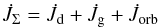 (1)where
 and
and  are the torques applied to the orbit, donor and gainer star, respectively. The stellar
torques that act on the stellar spins account for the action of tides (synchronization) and
change in AM due to the accretion or loss of mass. Note that in all the simulations, we
consider solid-body rotation and assume the initial stars to be (pseudo-)synchronized. The
evolution of the semi-major axis (a) is given by
are the torques applied to the orbit, donor and gainer star, respectively. The stellar
torques that act on the stellar spins account for the action of tides (synchronization) and
change in AM due to the accretion or loss of mass. Note that in all the simulations, we
consider solid-body rotation and assume the initial stars to be (pseudo-)synchronized. The
evolution of the semi-major axis (a) is given by 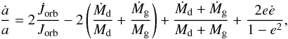 (2)where
 is evaluated from Eq. (1) and Ṁi =
d,g corresponds to the net1 mass change rate of star i. RLOF mass transfer rates are computed according to
the Kolb & Ritter (1990) prescription and the
Eggleton (1983) formulation for the Roche lobe
radius (RL1) is used.
is evaluated from Eq. (1) and Ṁi =
d,g corresponds to the net1 mass change rate of star i. RLOF mass transfer rates are computed according to
the Kolb & Ritter (1990) prescription and the
Eggleton (1983) formulation for the Roche lobe
radius (RL1) is used.
Changes in the eccentricity (e) due to the tidal interaction of each star
(ėtide,i) are calculated
from Zahn (1977, 1989) (for details, see Siess et al. 2013,
hereafter Paper I). However in an eccentric orbit, the specific AM of the ejected material
depends on the star’s position along its orbit and is potentially able to generate some
eccentricity. Following Soker (2000)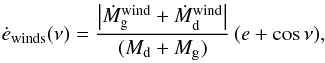 (3)where
ν is the true
anomaly and
(3)where
ν is the true
anomaly and  the wind mass loss rate from star i, assumed in these calculations to follow the Reimers (1975) prescription. The total rate of change of
the eccentricity is given by
the wind mass loss rate from star i, assumed in these calculations to follow the Reimers (1975) prescription. The total rate of change of
the eccentricity is given by  (4)The
specific AM of the wind material ejected from the system is assumed to be equal to the
specific orbital AM of the star at its position on the orbit, i.e.
(4)The
specific AM of the wind material ejected from the system is assumed to be equal to the
specific orbital AM of the star at its position on the orbit, i.e.  (5)where
ω is the
orbital angular velocity, ai the distance of star
i to the
center of mass of the system (a1 + a2 =
a), q =
Md/Mg
the mass ratio and jorb = Jorb/
(Md + Mg) the
specific orbital AM.
(5)where
ω is the
orbital angular velocity, ai the distance of star
i to the
center of mass of the system (a1 + a2 =
a), q =
Md/Mg
the mass ratio and jorb = Jorb/
(Md + Mg) the
specific orbital AM.
When the mass exchange rate depends on the orbital phase, as is the case in an eccentric
orbit for the RLOF mass transfer rate and tidally enhanced stellar winds (see Sect. 4.2), averaged quantities must be used in order to follow
the secular evolution of the system over millions of orbits. To achieve this goal, we use a
Gaussian quadrature integration scheme which involves the calculation of the mass transfer
properties at very specific locations (i.e. at given true anomalies) along the orbit. Once
the instantaneous Roche radius is known, at that orbital phase one can calculate the tidal
torques (ėtide,i) and the mass
transfer rates (either due to RLOF or tidally enhanced wind) from which the “local” values
of ėwinds and
 are derived. The mean quantities ⟨
Ṁi ⟩, ⟨ ėwinds ⟩ and
⟨
ȧ/a ⟩ are then
simply calculated by summing the weighted contribution of each variable at the specified
points. Technically, this resumes to calculating for X = {
Ṁ, ė, ȧ
}
are derived. The mean quantities ⟨
Ṁi ⟩, ⟨ ėwinds ⟩ and
⟨
ȧ/a ⟩ are then
simply calculated by summing the weighted contribution of each variable at the specified
points. Technically, this resumes to calculating for X = {
Ṁ, ė, ȧ
} where
νi and wi are tabulated
coefficients2.
where
νi and wi are tabulated
coefficients2.
3. Observational and evolutionary constraints
Merle et al. (2014) derive the first orbital
solution for IP Eri (=HD 18131 = EUVE J0254-053), a K0IV + DA WD system with P = 1071.00 ± 0.07 d and
e = 0.25 ±
0.01. An analysis of the WD atmospheric lines by Burleigh et al. (1997) and Vennes et al.
(1998) yielded an effective temperature of ~30 000 K and gravity log g ~ 7.5. These values,
combined with structural models and a revised Hipparcos distance estimate of ~ pc, leads to a mass close to 0.4 ± 0.03
M⊙ for the hot companion, implying that the
WD is made of He and not of carbon-oxygen. The stellar metallicity of the K0 giant is close
to solar with [Fe/H] ~ 0.1, with
an effective temperature Teff = 4960 ± 100 K and log g = 3.3 ± 0.3. These
parameters indicate that the star is located at the base of the RGB in the
Hertzsprung-Russell diagram (HRD) and its initial mass ranges between 1.2−1.3 ≲
Mgiant/M⊙ ≲
3. The low system mass function (f = 0.0036 M⊙) only sets an
upper limit on Mgiant <
4.26 M⊙. A detailed chemical analysis of the
giant reveals no s-process enhancement, implying that the WD progenitor avoided the
asymptotic giant branch (AGB) phase, consistent with its He composition. No sign of fast
rotation was detected in the giant with vsini < 5 km
s-1.
pc, leads to a mass close to 0.4 ± 0.03
M⊙ for the hot companion, implying that the
WD is made of He and not of carbon-oxygen. The stellar metallicity of the K0 giant is close
to solar with [Fe/H] ~ 0.1, with
an effective temperature Teff = 4960 ± 100 K and log g = 3.3 ± 0.3. These
parameters indicate that the star is located at the base of the RGB in the
Hertzsprung-Russell diagram (HRD) and its initial mass ranges between 1.2−1.3 ≲
Mgiant/M⊙ ≲
3. The low system mass function (f = 0.0036 M⊙) only sets an
upper limit on Mgiant <
4.26 M⊙. A detailed chemical analysis of the
giant reveals no s-process enhancement, implying that the WD progenitor avoided the
asymptotic giant branch (AGB) phase, consistent with its He composition. No sign of fast
rotation was detected in the giant with vsini < 5 km
s-1.
Given the mass of the He WD, its progenitor must have been less massive than 3 M⊙ initially, because stars of higher masses leave the main sequence with a H-depleted core more massive than the derived WD mass. We also inferred from single-star calculations performed with STAREVOL, that the age of the He WD on its cooling track is ≈107 yr.
Evolutionary timescales also impose some constraints on the mass of the WD progenitor. If we consider the system to be ~5 Gyr old, compatible with its solar-like composition, this imposes the mass-losing star to be at least ~1.2−1.3 M⊙, so that it can reach the RGB and start losing mass in that time interval.
Furthermore, the initial mass ratio must be close to unity so that, by the time the He WD forms and reaches its observed position in the HRD, the companion star has evolved substantially off the main sequence to comply with the observed values.
4. Stable RLOF channel
4.1. Circular systems
We start by investigating the stable RLOF channel, first for circular systems (Sect. 4.1) and then for eccentric ones (Sect. 4.2). The key point in this approach is to start with a binary having a mass ratio just above unity, so that when RLOF starts, q rapidly drops below unity ensuring stable mass transfer. The initial orbital period is chosen in such a way that the donor star fills its Roche lobe on the RGB. A set of evolutionary tracks has been computed for systems with initial masses M1 = 1.2 and M2 = 1.0 M⊙ and initial periods of 30, 100, 200 and 365 d.
As shown in Fig. 1, the final orbital periods range from 200 to 1400 d, covering the observed value. With increasing initial periods, mass transfer starts at higher luminosities corresponding to larger core masses. As a consequence, the mass of He WD increases from 0.34 M⊙ to 0.44 M⊙. In all simulations, the mass-transfer rate peaks around 10-2 M⊙ yr-1, decreases once the mass ratio has been reversed and then stabilizes around 10-8 M⊙ yr-1. We note that the phase of rapid mass transfer (Ṁ > 10-5 M⊙ yr-1) occurs over a larger mass range if RLOF starts later in the evolution. The reason for this behavior is because, as the star climbs the RGB, the energy demand from the H-burning shell (HBS) increases. To compensate for the higher radiative losses from the surface, H is burnt at a higher rate and the core growth rate (ṀHBS) increases. Because the expansion of the star is driven by the HBS, a higher ṀHBS leads to a larger overfilling factor (R/RL1) and hence mass-transfer rate. When all the envelope is removed, the star leaves the RGB and moves to the blue as the hot He core is progressively exposed. Our simulations can reproduce the observed period and WD mass of IP Eri provided the system had an initial period of ≈300 days.
The evolution of the secondary component is not very sensitive to the initial period. It lands on the main sequence with a mass on the order of 1.6–1.7 M⊙ when a conservative evolution is considered. As described at the end of Sect. 5, some fine tuning is required to match the position in the HR diagram for both stars. It is also worth noticing that in this process, the accretion of AM spins up the gainer close to its breakup velocity which is incompatible with observations.
 |
Fig. 1 Evolution of the semi-major axis (top), mass-transfer rate (mid) and period (bottom, in days) for the circular RLOF systems as a function of the donor’s mass. The curves correspond to different initial orbital periods: 30 (solid, black), 100 (red, dotted), 200 (green, short-dashed) and 365 days (blue, long-dashed). The initial masses are 1.2 + 1.0 M⊙. |
4.2. Eccentric systems
If we now consider a system with an initial eccentricity e = 0.3 and re-perform the
previous calculations, we find that in all cases, the orbit has circularized by the time
RLOF starts. The reason is that mass transfer begins when the star has already evolved
along the giant branch and possesses a deep convective envelope. Convection is the most
efficient mechanism for dissipating the kinetic energy of the tidally-induced large-scale
flows (e.g. Zahn 2008). According to Zahn (1978), the circularization timescale can be
expressed as  (6)where
k2 is the apsidal motion constant and
(6)where
k2 is the apsidal motion constant and
 ,
the other quantities having their usual meanings. Inserting the Roche lobe radius
(RL1) formula of Paczyński (1971) in Eq. (6) and assuming q ≈
1 as required by our scenario, we find that
,
the other quantities having their usual meanings. Inserting the Roche lobe radius
(RL1) formula of Paczyński (1971) in Eq. (6) and assuming q ≈
1 as required by our scenario, we find that
 yr which is
extremely short in comparison to the evolutionary (Kelvin-Helmholtz) timescale along the
RGB. Therefore, as the star expands and progressively fills its Roche lobe, the orbit
circularizes before RLOF had even started. So, within this paradigm, it is impossible to
prevent the circularization of the orbit, at least for the low- and intermediate-mass
stars that we consider.
yr which is
extremely short in comparison to the evolutionary (Kelvin-Helmholtz) timescale along the
RGB. Therefore, as the star expands and progressively fills its Roche lobe, the orbit
circularizes before RLOF had even started. So, within this paradigm, it is impossible to
prevent the circularization of the orbit, at least for the low- and intermediate-mass
stars that we consider.
5. The enhanced wind scenario
The only solution to form a He WD and preserve some eccentricity is to remove mass from the
giant while keeping it well inside its Roche radius so that the tidal effects remain weak.
One possibility to meet these requirements is to boost the wind mass-loss rate prior to RLOF
as proposed by Tout & Eggleton (1988). In
their model, the authors advocate that tidal interactions and/or magnetic activity are
responsible for the stellar wind enhancement and assume that the multiplying factor has the
same dependence on the radius and separation as the tidal torque applied onto that star.
This lead Tout & Eggleton (1988) to propose
the following expression for the mass-loss rate ![Mathematical equation: \begin{eqnarray} \dot{M}^\mathrm{wind}_i = \dot{M}_i^\mathrm{Reimers}\times \Biggl\{1+B_\mathrm{wind}\times \min\biggl[\biggl(\frac{R}{R_{\rm L1}}\biggr)^6,\frac{1}{2^6}\biggl]\Biggl\}, \label{eq:mloss} \end{eqnarray}](/articles/aa/full_html/2014/05/aa23397-14/aa23397-14-eq69.png) (7)where
ṀReimers is the Reimers’ mass-loss rate and
the constant Bwind =
104 was found to match the properties of Z Her, a RS CVn
system with a mass ratio below unity.
(7)where
ṀReimers is the Reimers’ mass-loss rate and
the constant Bwind =
104 was found to match the properties of Z Her, a RS CVn
system with a mass ratio below unity.
The results of our new simulations including the tidally enhanced wind are depicted in Fig. 2 (we use the same initial conditions as in the previous section). Several points draw our attention: first, this mechanism leads to smaller He WD masses because, for a given initial period, the envelope is removed faster (to prevent the radius from approaching RL1 too closely) which in turn leaves less time for the H-burning shell to advance outward. Second, the higher amount of mass lost by the system reduces the final separation compared to the previous (conservative) RLOF evolution. For example, in the RLOF calculation, the one-year initial-period system leads to the formation of a 1400 d period system with a 0.43 M⊙ He WD. For the enhanced wind prescription, we obtain a 0.36 M⊙ He WD binary in a 850 d orbital period. This implies that in order to reproduce the observed period of IP Eri, a larger initial separation must be selected.
However, the most interesting feature is the preservation and even increase of the
eccentricity in the long-period systems. We remark that, if the initial separation is less
than ~200 d for our 1.2 + 1.0
M⊙
system, the mass-loss rate enhancement occurs too early, when
 is relatively low. As a consequence, the eccentricity pumping term (ėwinds) in Eq.
(4) remains small, | ėtides |
dominates and the eccentricity globally decreases. Thus, there exists a critical initial
period above which ėwinds > |
ėtides | and eccentricity can be preserved
but its analytical derivation is not straightforward because of the dependence of the mass
loss rate on the eccentricity (via the determination of the Roche radius) and the simplistic
approach of Soker (2000), which assumes a constant
mass-loss rate independent of the orbital phase, cannot be reiterated here.
is relatively low. As a consequence, the eccentricity pumping term (ėwinds) in Eq.
(4) remains small, | ėtides |
dominates and the eccentricity globally decreases. Thus, there exists a critical initial
period above which ėwinds > |
ėtides | and eccentricity can be preserved
but its analytical derivation is not straightforward because of the dependence of the mass
loss rate on the eccentricity (via the determination of the Roche radius) and the simplistic
approach of Soker (2000), which assumes a constant
mass-loss rate independent of the orbital phase, cannot be reiterated here.
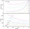 |
Fig. 2 Evolution of the eccentricity (top) and orbital period (bottom, in days) for the enhanced-wind models as a function of the donor’s mass. The curves correspond to different initial orbital periods: 30 (solid, black), 100 (red, dotted), 200 (green, short-dashed) days, 1 (blue, long-dashed), 1.5 (cyan, dot-short dashed) and 2 years (magenta, dot-long dashed). The initial stellar masses are 1.2 + 1.0 M⊙. |
However, the final eccentricity still remains lower than the observed value. To improve the situation, we explored the parameter space, first varying the initial mass ratio and eccentricity. The results are presented in Fig. 3 and show the absence of any obvious relation between the initial and final eccentricities. In particular, a system initially more eccentric will not necessarily end up with a higher final eccentricity and the reason is because quantities are averaged over an orbit. For a given initial period, with increasing eccentricity, the stars get closer to each other at periastron. On one hand, this contributes to further enhance the mass-loss rate due to its strong dependence on the Roche radius (which depends on the instantaneous separation) and hence ėwinds but on the other hand, the star spends a longer fraction of its time at greater distances, where the wind is weak. The result is that the mean wind mass-loss rate decreases with increasing eccentricity, leading to less efficient eccentricity pumping and in the end to a stronger circularization of the orbit. Due to the nonlinearity of these effects, this conclusion may, however, depend on the initial configuration.
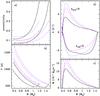 |
Fig. 3 Evolution of the eccentricity a), orbital period b), wind mass loss rate c) and ė contributions d) as a function of the donor’s mass under various physical configurations. The initial period is the same for all simulations and equal to 550 days. The three curves in panel a) and b) starting at M = 1.5 M⊙ show the evolution of a 1.5 + 1.0 M⊙ system for initial eccentricities equal to 0.5 (black, solid), 0.3 (blue, dotted) and 0.2 (red, short-dashed). The evolution of a 1.2 + 1.0 M⊙ system with same initial eccentricities is also shown with the same line coding but different colors. In the right panels, only the properties of the 1.5 + 1.0 M⊙ system are shown. The positive ė corresponds to the pumping term, the negative part to the tidal one. |
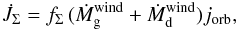
Given the uncertainties in the initial-system mass ratio, we performed several simulations,
starting with the same initial period of 550 days and varying q. All mass-losing stars end
up with about the same WD mass between 0.37 and 0.43 M⊙. From the
curves depicted in Fig. 4, we see that increasing the
donor’s mass for a given companion mass leads to longer final period (green vs. blue curve)
because in this nonconservative evolution, a larger amount of mass has been removed from the
system to form the He WD (this response of the orbital parameters to systemic mass loss is
demonstrated in the appendix). If we now fix the mass of the WD progenitor but increase that
of the companion (cyan vs. red curve), the systems evolve toward shorter final periods. In
these configurations about the same mass is ejected from the system but, in the binaries
with the higher mass companion, a much larger amount of AM will be taken away by the wind
because the specific AM of the ejected material (Eq. (5)) increases with increasing system mass
( )
and decreasing mass ratio.
)
and decreasing mass ratio.
Finally, systems with similar mass ratios (red and black curves) evolve along the same q vs. Porb trajectory as demonstrated in the appendix (Eq. (A.6)). This is a consequence of our prescription for the systemic AM loss rate (Eq. (5)) and of the fact that the gainer is not accreting mass. As discussed previously, the final periods lengthen with increasing donor mass.
The final eccentricity (which in Fig. 4 always ends up
being too small with respect to IP Eri observed value) is dictated by the competition
between ėwinds and ėtides and, for a
given initial period, depends mostly on the donor’s initial mass because the ė contributions are imposed
by the mass-losing star (ėtide,d ≫
ėtide,g and
 responsible for ėwinds). We also notice that systems with
higher initial masses require larger initial separations to avoid RLOF. Consequently, they
end their evolution at much longer periods that are incompatible with observations.
responsible for ėwinds). We also notice that systems with
higher initial masses require larger initial separations to avoid RLOF. Consequently, they
end their evolution at much longer periods that are incompatible with observations.
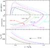 |
Fig. 4 Evolution of the wind-enhancement factor (top), eccentricity (mid) and period (bottom) as a function of the mass ratio for the different initial configurations specified in the graph. All systems have an initial period of 550 d and an eccentricity e = 0.3. The arrow indicates the current orbital period of IP Eri. Note the saturation of the mass-loss rate in the 2.0+1.9 M⊙ system (top panel). |
Among the various parameters influencing the final orbital period, the amount of AM lost by
the wind is an important one. By default we assume that the wind carries away the orbital
angular momentum of the star at its position on the orbit (Eq. (5)). In an alternative set of model calculations
depicted in Fig. 5, we use the prescription described
by Eq. (37) of Siess et al. (2013):
 (8)where
fΣ
is a free parameter encapsulating our ignorance of the exact mode of AM ejection. With
decreasing values of this parameter, the wind removes less AM from the system.
Jorb is consequently larger, the separation
larger and the tidal torques weaker. The system is thus able to keep a higher eccentricity
and the separation keeps increasing as a result of nonconservative evolution, but to an
extent that is no longer compatible with the observations (see for example the cases with
fΣ =
0.3 or 1 in Fig. 5). If instead we
set fΣ =
2.0, the period remains within the observed value but because of the
shorter separation, the eccentricity is substantially reduced. So this alternative
prescription for
(8)where
fΣ
is a free parameter encapsulating our ignorance of the exact mode of AM ejection. With
decreasing values of this parameter, the wind removes less AM from the system.
Jorb is consequently larger, the separation
larger and the tidal torques weaker. The system is thus able to keep a higher eccentricity
and the separation keeps increasing as a result of nonconservative evolution, but to an
extent that is no longer compatible with the observations (see for example the cases with
fΣ =
0.3 or 1 in Fig. 5). If instead we
set fΣ =
2.0, the period remains within the observed value but because of the
shorter separation, the eccentricity is substantially reduced. So this alternative
prescription for  cannot at the same time increase the eccentricity and maintain the period close to
~103 d.
cannot at the same time increase the eccentricity and maintain the period close to
~103 d.
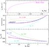 |
Fig. 5 Evolution of the surface spin velocity of the gainer as a function of its mass (top, with fjacc = 0.1) and of the eccentricity (mid) and period (bottom) as a function of the donor’s mass under different physical assumptions as specified in the graph. The initial configuration is a 1.2 + 1.0 M⊙ system, with an initial period of 550 d and an eccentricity e = 0.3 (see text for details). |
So far, we have neglected the possibility that a fraction of the tidally-enhanced wind
could be captured by the companion. In a first simulation, we used the classical Bondi-Hoyle
wind-accretion scheme where the default wind parameters of Eq. (25) of Paper I are adapted
to the slow (≲20 km
s-1) wind of the
giant ( and
αBH =
0.15 instead of
and
αBH =
0.15 instead of  and 1.5
respectively as suggested by Hurley et al. (2002) for
classical Bondi-Hoyle accretion rates). Following Shapiro
& Lightman (1976) and Jeffries &
Stevens (1996), we approximate the torque exerted by the wind onto the gainer by
and 1.5
respectively as suggested by Hurley et al. (2002) for
classical Bondi-Hoyle accretion rates). Following Shapiro
& Lightman (1976) and Jeffries &
Stevens (1996), we approximate the torque exerted by the wind onto the gainer by
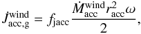 (9)where
fjacc is a free parameter set to 0.1 as
suggested by Jeffries & Stevens (1996). The
gainer’s accretion radius is given by
(9)where
fjacc is a free parameter set to 0.1 as
suggested by Jeffries & Stevens (1996). The
gainer’s accretion radius is given by
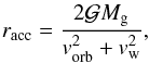 (10)where
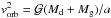 is the orbital velocity and
vw
the wind velocity set to a fraction βw of the star’s escape velocity.
is the orbital velocity and
vw
the wind velocity set to a fraction βw of the star’s escape velocity.
Accounting for wind accretion does not significantly alter the global picture because little AM is deposited on the gainer. The main observable effect is an increase of the companion’s rotation rate. For reasonable values of the parameters as used in this test simulation, the gainer accelerates up to 20 km s-1, which is not so far off the observed value. It is important to emphasize that the enhanced wind scenario avoids the problem associated with the critical rotation of the gainer star when mass is transferred via RLOF (Packet 1981; Dervişoğlu et al. 2010; Deschamps et al. 2013).
As a final test, we also varied the wind parameter Bwind. This
parameter is badly constrained and is likely to depend on the structure of the star and vary
with time. Considering these large uncertainties (including the ad hoc dependence of Eq.
(7) on R/RL1),
we calculated a new model using the standard physics (i.e.
given by Eq. (5) and no wind accretion) but
with Bwind = 2 ×
104 (Fig. 5, red
curve). As expected, because of the stronger wind, the eccentricity-pumping mechanism is
more efficient leading to a final eccentricity of ~0.23 in very good agreement with the observed value for IP Eri. This
doubling of the wind mass-loss rate has little impact on the orbital period which is very
similar to our default case.
Finally, Fig. 6 depicts the temporal evolution of some
key observable parameters for the model calculation (initial masses of 1.5 + 1.45 M⊙, initial period
of 415 d, initial eccentricity of 0.4, Bwind = 3.6 × 10⁴,
αBH =
0.1, ,
fjacc =
0.03 and Eq. (5) for
)
best reproducing the current values of the system IP Eri. The agreement is remarkable
considering that we are able to fit at once 7 observational constraints. We note however
that the mass of the He WD (0.35 M⊙) is slightly below the value inferred
from model atmosphere fitting of the WD spectrum. A better agreement could in principle be
achieved if some core overshooting is operating in the giant but one should also be aware
that the procedure used to determine the WD mass suffers its own limitations and
uncertainties. Finally, the slow rotation of the K0 giant can only be fitted if
fjacc =
0.03 implying that little AM must be accreted.
6. Discussion
The formation of a He WD requires a binary system in which the evolution of one of the components is truncated before it reaches the tip of the RGB. Three main evolutionary channels can lead to a binary system hosting a He WD and a main sequence or giant star:
-
1.
unstable RLOF mass transfer. If the initial mass ratio exceedsqcrit ≳ 1.2−1.5, the mass transfer is dynamical and the system most likely enters a common-envelope phase where the eccentricity is reduced to zero and the period is considerably shortened;
-
2.
RLOF mass transfer is stable because initially q<qcrit. The system avoids a catastrophic evolution and ends up as a long-period binary in a circular orbit;
-
3.
the initially most massive star ejected its envelope due to enhanced stellar winds and RLOF is avoided. If the period is long enough, eccentricity is preserved or can even be increased.
The properties of IP Eri, a system consisting of a giant K0 and a He WD with a period of 1071 d and an eccentricity of 0.23, can only be explained by the tidally-enhanced wind model, i.e. via scenario 3 mentioned above. Our exploration of this evolutionary channel indicates that there is a critical period below which eccentricity decrease due to tidal effects will always dominate over the eccentricity pumping due to the wind mass loss. But such a limit is difficult to determine without an extensive exploration of the parameter space. As presented in Sect. 3, this scenario also imposes some constraints on the initial mass ratio of IP Eri. It must not be too far above unity so that in the relatively short time interval during which the envelope is stripped and the WD cooled down, the initially lower-mass companion star has left the main sequence and started to climb the RGB. We also showed that (1) only stars less massive than 3 M⊙ may give birth to a He WD (see Sect. 3); and (2) at solar metallicity, Md ≳ 1.2 M⊙ for the He WD to form within 5 Gyr.
In contrast to the related Wind-Induced Rapidly-Rotating (WIRRING) systems like 2RE J0357+283 (Jeffries & Stevens 1996), the slow angular velocity of the K0 giant in IP Eri indicates that little angular momentum has been accreted in the He-WD formation process (fjacc = 0.03). The main reason for this difference is that in their model, Jeffries & Stevens (1996) consider the ejection of a massive AGB envelope and impose a significantly higher wind mass-loss rate (>10-5 M⊙ yr-1). They also restrict their study to circular systems, assume a constant AGB wind mass-loss rate and do not follow the evolution of the structure of the stellar components which for our RGB is significant. Indeed, during the tidally-enhanced mass-loss phase, the radius of the giant increases by more than a factor 4 (see Fig. 6), reaching up to 40–60 R⊙ before leaving the RGB. All these effects result in larger amounts of mass and AM being accreted by the companion of the AGB star which is spun up to much higher rotational velocities.
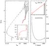 |
Fig. 6 Temporal evolution of some key observable parameters for the model calculation
(initial masses of 1.5 +
1.45 M⊙, initial period of 415 d,
e =
0.4, Bwind = 3.6 × 10⁴,
αBH =
0.1, |

The tidally-enhanced wind model implies that a substantial amount of mass must be removed from the system. This mass may give rise to a large IR excess. However, by the time the He WD is observed (some 107 yr after the end of the envelope ejection phase for our 1.2+1.0 M⊙ system), this material has long since been dispersed and mixed with the interstellar medium, making its detection difficult.
Scenarios 1 and 2 above most likely produce circular systems because of tidal effects acting before and during RLOF, unless some eccentricity can be generated either via the interaction between a circumbinary disc and the orbit (Goldreich & Tremaine 1979; Artymowicz & Lubow 1994; Dermine et al. 2012) or because of asymmetric mass loss (Soker 2000; Frankowski & Tylenda 2001).
The detection of He-WD + MS or giant binaries, and more recently of sdBs, with long periods and high eccentricities, support the tidally-enhanced wind model which is otherwise often advocated to explain the evolution of a handful of additional systems, including some RS CVn binaries, Algols and Barium stars as reviewed by Eggleton & Tout (1989). However the source of eccentricity may differ between these systems. For example the presence of a circumbinary disc (Goldreich & Tremaine 1979; Artymowicz & Lubow 1994; Dermine et al. 2012) could act in place or in parallel to the asymmetric mass loss mechanism.
Clearly this tidally-enhanced wind model provides a simple framework to reproduce the observed properties of IP Eri but such studies need to be extended to different classes of objects, in order to better constrain the parameters of our models and understand the source of this puzzling eccentricity.
This includes contributions from mass accretion/loss via RLOF and/or wind.
Acknowledgments
This work has been partly funded by an Action de recherche concerte (ARC) from the Direction générale de l’Enseignement non obligatoire et de la Recherche scientifique – Direction de la recherche scientifique – Communauté française de Belgique. L.S. is research associate at the F.R.S.-FNRS. P.J.D. is Senior Research Assistant at F.R.S.-FNRS.
References
- Artymowicz, P., & Lubow, S. H. 1994, ApJ, 421, 651 [NASA ADS] [CrossRef] [Google Scholar]
- Barlow, B. N., Wade, R. A., Liss, S. E., Østensen, R. H., & Van Winckel, H. 2012, ApJ, 758, 58 [NASA ADS] [CrossRef] [Google Scholar]
- Barlow, B. N., Liss, S. E., Wade, R. A., & Green, E. M. 2013, ApJ, 771, 23 [NASA ADS] [CrossRef] [Google Scholar]
- Burleigh, M. R., Barstow, M. A., & Fleming, T. A. 1997, MNRAS, 287, 381 [NASA ADS] [CrossRef] [Google Scholar]
- Clausen, D., & Wade, R. A. 2011, ApJ, 733, L42 [NASA ADS] [CrossRef] [Google Scholar]
- Davis, P. J., Siess, L., & Deschamps, R. 2013, A&A, 556, A4 [NASA ADS] [CrossRef] [EDP Sciences] [Google Scholar]
- Deca, J., Marsh, T. R., Østensen, R. H., et al. 2012, MNRAS, 421, 2798 [NASA ADS] [CrossRef] [Google Scholar]
- Dermine, T., Izzard, R. G., Jorissen, A., & Van Winckel, H. 2012, unpublished [arXiv:1203.6471] [Google Scholar]
- Dervişoğlu, A., Tout, C. A., & Ibanoğlu, C. 2010, MNRAS, 406, 1071 [NASA ADS] [Google Scholar]
- Deschamps, R., Siess, L., Davis, P. J., & Jorissen, A. 2013, A&A, 557, A40 [NASA ADS] [CrossRef] [EDP Sciences] [Google Scholar]
- Eggleton, P. P. 1983, ApJ, 268, 368 [NASA ADS] [CrossRef] [Google Scholar]
- Eggleton, P. P., & Tout, C. A. 1989, Space Sci. Rev., 50, 165 [NASA ADS] [CrossRef] [Google Scholar]
- Frankowski, A., & Tylenda, R. 2001, A&A, 367, 513 [NASA ADS] [CrossRef] [EDP Sciences] [Google Scholar]
- Goldreich, P., & Tremaine, S. 1979, ApJ, 233, 857 [NASA ADS] [CrossRef] [MathSciNet] [Google Scholar]
- Han, Z., Podsiadlowski, P., Maxted, P. F. L., Marsh, T. R., & Ivanova, N. 2002, MNRAS, 336, 449 [NASA ADS] [CrossRef] [Google Scholar]
- Han, Z., Podsiadlowski, P., Maxted, P. F. L., & Marsh, T. R. 2003, MNRAS, 341, 669 [NASA ADS] [CrossRef] [Google Scholar]
- Heber, U. 1986, A&A, 155, 33 [NASA ADS] [Google Scholar]
- Hurley, J. R., Tout, C. A., & Pols, O. R. 2002, MNRAS, 329, 897 [NASA ADS] [CrossRef] [Google Scholar]
- Jeffries, R. D., & Stevens, I. R. 1996, MNRAS, 279, 180 [NASA ADS] [CrossRef] [Google Scholar]
- Kolb, U., & Ritter, H. 1990, A&A, 236, 385 [NASA ADS] [Google Scholar]
- Landsman, W., Simon, T., & Bergeron, P. 1993, PASP, 105, 841 [NASA ADS] [CrossRef] [Google Scholar]
- Merle, T., Jorissen, A., Masseron, T., et al. 2014, A&A, submitted [Google Scholar]
- Nelemans, G. 2010, Ap&SS, 329, 25 [NASA ADS] [CrossRef] [Google Scholar]
- Nelemans, G., & Tout, C. A. 2005, MNRAS, 356, 753 [NASA ADS] [CrossRef] [Google Scholar]
- Østensen, R. H., & Van Winckel, H. 2011, in Evolution of Compact Binaries, eds. L. Schmidtobreick, M. R. Schreiber, & C. Tappert, ASP Conf. Ser., 447, 171 [Google Scholar]
- Østensen, R. H., & Van Winckel, H. 2012, in Fifth Meeting on Hot Subdwarf Stars and Related Objects, eds. D. Kilkenny, C. S. Jeffery, & C. Koen, ASP Conf. Ser., 452, 163 [Google Scholar]
- Packet, W. 1981, A&A, 102, 17 [NASA ADS] [Google Scholar]
- Paczyński, B. 1971, ARA&A, 9, 183 [NASA ADS] [CrossRef] [Google Scholar]
- Podsiadlowski, P., Han, Z., Lynas-Gray, A. E., & Brown, D. 2008, in Hot Subdwarf Stars and Related Objects, eds. U. Heber, C. S. Jeffery, & R. Napiwotzki, ASP Conf. Ser., 392, 15 [Google Scholar]
- Reimers, D. 1975, Mém. Soc. Roy. Sci. Liège, 8, 369 [Google Scholar]
- Shapiro, S. L., & Lightman, A. P. 1976, ApJ, 204, 555 [NASA ADS] [CrossRef] [Google Scholar]
- Siess, L. 2006, A&A, 448, 717 [NASA ADS] [CrossRef] [EDP Sciences] [Google Scholar]
- Siess, L., Izzard, R. G., Davis, P. J., & Deschamps, R. 2013, A&A, 550, 100 (Paper I) [Google Scholar]
- Soberman, G. E., Phinney, E. S., & van den Heuvel, E. P. J. 1997, A&A, 327, 620 [NASA ADS] [Google Scholar]
- Soker, N. 2000, A&A, 357, 557 [NASA ADS] [Google Scholar]
- Tout, C. A., & Eggleton, P. P. 1988, MNRAS, 231, 823 [NASA ADS] [CrossRef] [Google Scholar]
- Vennes, S., Christian, D. J., & Thorstensen, J. R. 1998, ApJ, 502, 763 [NASA ADS] [CrossRef] [Google Scholar]
- Vos, J., Østensen, R. H., Degroote, P., et al. 2012, A&A, 548, A6 [NASA ADS] [CrossRef] [EDP Sciences] [Google Scholar]
- Webbink, R. F. 1988, The Formation and Evolution of Symbiotic Stars, eds. J. Mikolajewska, M. Friedjung, S. J. Kenyon, & R. Viotti (Dordrecht: Kluwer Academic Publisher), 311 [Google Scholar]
- Zahn, J.-P. 1977, A&A, 57, 383 [NASA ADS] [Google Scholar]
- Zahn, J.-P. 1989, A&A, 220, 112 [NASA ADS] [Google Scholar]
- Zahn, J.-P. 2008, in EAS Pub. Ser., 29, eds. M.-J. Goupil, & J.-P. Zahn, 67 [Google Scholar]
- Zahn, J.-R. 1978, A&A, 67, 162 [NASA ADS] [Google Scholar]
Appendix A: Evolution of the period as function of the mass ratio
In the framework of the tidally-enhanced stellar wind model, the companion star accretes
almost no matter and the rate of change of the orbital AM is mainly due to the systemic AM
loss rate resulting from the giant’s wind. Under these circumstances,
 and Eq. (2) simplifies to
 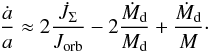 (A.1)With
q =
Md/Mg
and Ṁg =
0, Eq. (5) can be recast
into
(A.1)With
q =
Md/Mg
and Ṁg =
0, Eq. (5) can be recast
into 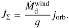 (A.2)Substituting
Eq. (A.2) into Eq. (A.1) leads to
(A.2)Substituting
Eq. (A.2) into Eq. (A.1) leads to  (A.3)This
last equation tells us that when systemic mass loss prevails and has the usual form of Eq.
(5), the orbital separation increases
independently of the mass ratio. Now using Kepler’s third law along with Eq. (A.3), we can relate the change in period
P to that
of the system’s mass
(A.3)This
last equation tells us that when systemic mass loss prevails and has the usual form of Eq.
(5), the orbital separation increases
independently of the mass ratio. Now using Kepler’s third law along with Eq. (A.3), we can relate the change in period
P to that
of the system’s mass 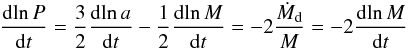 (A.4)and
with M = (1 +
q)Mg, one finally
obtains the relation
(A.4)and
with M = (1 +
q)Mg, one finally
obtains the relation  (A.5)which,
after integration leads to
(A.5)which,
after integration leads to  (A.6)where
P0 and q0 are the
initial period and mass ratio. This relation explains why, when systemic mass loss
dominates, the evolution of the period only depends on that of the mass ratio.
(A.6)where
P0 and q0 are the
initial period and mass ratio. This relation explains why, when systemic mass loss
dominates, the evolution of the period only depends on that of the mass ratio.
All Figures
|
Fig. 1 Evolution of the semi-major axis (top), mass-transfer rate (mid) and period (bottom, in days) for the circular RLOF systems as a function of the donor’s mass. The curves correspond to different initial orbital periods: 30 (solid, black), 100 (red, dotted), 200 (green, short-dashed) and 365 days (blue, long-dashed). The initial masses are 1.2 + 1.0 M⊙. |
| In the text | |
|
Fig. 2 Evolution of the eccentricity (top) and orbital period (bottom, in days) for the enhanced-wind models as a function of the donor’s mass. The curves correspond to different initial orbital periods: 30 (solid, black), 100 (red, dotted), 200 (green, short-dashed) days, 1 (blue, long-dashed), 1.5 (cyan, dot-short dashed) and 2 years (magenta, dot-long dashed). The initial stellar masses are 1.2 + 1.0 M⊙. |
| In the text | |
|
Fig. 3 Evolution of the eccentricity a), orbital period b), wind mass loss rate c) and ė contributions d) as a function of the donor’s mass under various physical configurations. The initial period is the same for all simulations and equal to 550 days. The three curves in panel a) and b) starting at M = 1.5 M⊙ show the evolution of a 1.5 + 1.0 M⊙ system for initial eccentricities equal to 0.5 (black, solid), 0.3 (blue, dotted) and 0.2 (red, short-dashed). The evolution of a 1.2 + 1.0 M⊙ system with same initial eccentricities is also shown with the same line coding but different colors. In the right panels, only the properties of the 1.5 + 1.0 M⊙ system are shown. The positive ė corresponds to the pumping term, the negative part to the tidal one. |
| In the text | |
|
Fig. 4 Evolution of the wind-enhancement factor (top), eccentricity (mid) and period (bottom) as a function of the mass ratio for the different initial configurations specified in the graph. All systems have an initial period of 550 d and an eccentricity e = 0.3. The arrow indicates the current orbital period of IP Eri. Note the saturation of the mass-loss rate in the 2.0+1.9 M⊙ system (top panel). |
| In the text | |
|
Fig. 5 Evolution of the surface spin velocity of the gainer as a function of its mass (top, with fjacc = 0.1) and of the eccentricity (mid) and period (bottom) as a function of the donor’s mass under different physical assumptions as specified in the graph. The initial configuration is a 1.2 + 1.0 M⊙ system, with an initial period of 550 d and an eccentricity e = 0.3 (see text for details). |
| In the text | |
|
Fig. 6 Temporal evolution of some key observable parameters for the model calculation
(initial masses of 1.5 +
1.45 M⊙, initial period of 415 d,
e =
0.4, Bwind = 3.6 × 10⁴,
αBH =
0.1, |
| In the text | |
Current usage metrics show cumulative count of Article Views (full-text article views including HTML views, PDF and ePub downloads, according to the available data) and Abstracts Views on Vision4Press platform.
Data correspond to usage on the plateform after 2015. The current usage metrics is available 48-96 hours after online publication and is updated daily on week days.
Initial download of the metrics may take a while.