| Issue |
A&A
Volume 565, May 2014
|
|
|---|---|---|
| Article Number | A72 | |
| Number of page(s) | 11 | |
| Section | Stellar structure and evolution | |
| DOI | https://doi.org/10.1051/0004-6361/201323361 | |
| Published online | 14 May 2014 | |
Optical and X-ray rest-frame light curves of the BAT6 sample⋆,⋆⋆
1 INAF − Osservatorio Astronomico di Brera, via Bianchi 46,
23807 Merate ( LC), Italy
e-mail:
This email address is being protected from spambots. You need JavaScript enabled to view it.
2
Università degli Studi di Milano-Bicocca,
Piazza della Scienza
3, 20126
Milano,
Italy
3
INAF − IASF Milano, via E. Bassini 15, 20133, Milano,
Italy
4
ASI− Science Data Center, via del Politecnico snc, 00133
Roma,
Italy
5 INAF − Osservatorio Astronomico di Roma, via Frascati 33,
00040 Monte Porzio Catone ( RM), Italy
6
APC, Univ. Paris Diderot, CNRS/IN2P3, CEA/Irfu,
Obs. de Paris, Sorbonne Paris
Cité, 75205
Paris,
France
7
GEPI, Observatoire de Paris, CNRS, Univ. Paris Diderot, 5 place Jule Janssen,
92190
Meudon,
France
Received: 31 December 2013
Accepted: 6 March 2014
Abstract
Aims. We present the rest-frame light curves in the optical and X-ray bands of an unbiased and complete sample of the Swift long gamma-ray bursts (GRBs), namely, the BAT6 sample.
Methods. The unbiased BAT6 sample (consisting of 58 events) has the highest level of completeness in redshift (~95%), allowing us to compute the rest-frame X-ray and optical light curves for 55 and 47 objects, respectively. We compute the X-ray and optical luminosities, which accounte for any possible source of absorption (Galactic and intrinsic) that could affect the observed fluxes in these two bands.
Results. We compare the behaviour observed in the X-ray to that in the optical bands to assess the relative contribution of the emission during the prompt and afterglow phases. We unarguably demonstrate that rest-frame optical luminosity distribution of the GRBs is not bimodal and is clustered around the mean value Log(LR) = 29.9 ± 0.8 when estimated at a rest-frame time of 12 h. This is in contrast to what is found in previous works and confirms that the GRB population has an intrinsic unimodal luminosity distribution. For more than 70% of the events, the rest-frame light curves in the X-ray and optical bands have a different evolution, indicating distinct emitting regions and/or mechanisms. The X-ray light curves, which are normalised to the GRB isotropic energy (Eiso), provide evidence for X-ray emission that is still powered by the prompt emission until late times (~hours after the burst event). On the other hand, the same test performed for the Eiso-normalised optical light curves shows that the optical emission is a better proxy of the afterglow emission from early to late times.
Key words: gamma-ray burst: general / gamma rays: general / X-rays: general
Appendix A is available in electronic form at http://www.aanda.org
Tables 2 and 3 and data used for the figures are only available at the CDS via anonymous ftp to cdsarc.u-strasbg.fr (130.79.128.5) or via http://cdsarc.u-strasbg.fr/viz-bin/qcat?J/A+A/565/A72
© ESO, 2014
1. Introduction
In the past few years, the advances in detecting, fast re-pointing and observing gamma-ray bursts (GRBs) by the Swift satellite (Gehrels et al. 2004) has allowed the creation of uniform collections of events for statistical purposes (Nousek et al. 2006; Zhang et al. 2006; Gehrels et al. 2008; Evans et al. 2009; Roming et al. 2009; Oates et al. 2009; Kann et al. 2006, 2011; Rykoff et al. 2009; Nysewander et al. 2009; Li et al. 2012; Melandri et al. 2008; Liang et al. 2012; Salvaterra et al. 2012; Margutti et al. 2013). Depending on the selection criteria defining the sample, these collections of GRBs probe the parameter space of rest-frame time-brightness in a different manner. Among the samples collected, the most complete sample of bright Swift GRBs is the one by Salvaterra et al. (2012), where the selection of bright events in the γ-ray band has led to an homogeneous set of GRBs with very good coverage of the X-ray and optical bands, which also gives a completeness in redshift of ~95%.
The exploitation of this complete sample has give us some interesting statistical results to the overall class of bright GRBs for the first time: a) a strong evolution of the luminosity or density distribution has been needed to account for the observations (Salvaterra et al. 2012); b) selection effects have been negligible in shaping the spectral-energy correlations that might be due to a strong physical mechanism common to large majority of GRBs (Nava et al. 2012; Ghirlanda et al. 2012); c) the existence of a true population of dark GRBs that generate in much denser environments (Melandri et al. 2012) has been determined ; d) a strong correlation between GRB darkness and X-ray absorbing column densities (Campana et al. 2012) has been found; e) a significant correlation between X-ray luminosity and prompt γ-ray energy and luminosity (D’Avanzo et al. 2012) has been found; f) a distribution of rest-frame absorption coefficients has peaked at low values with a tail of dark GRB highly absorbed (Covino et al. 2013).
In this paper, we finally investigate the properties of the rest-frame optical luminosity of the complete BAT6 sample (details about the selecting criteria of the sample in Salvaterra et al. 2012) by showing and comparing the rest-frame light curves of each event in the γ-ray, X-ray and optical bands. Throughout the paper we assume a standard cosmology with H0 = 72 km s-1 Mpc-1, Ωm = 0.27, and ΩΛ = 0.73.
2. Luminosity light-curve fits
We followed the classification scheme described in Margutti et al. (2013) that divided the light curves in four main classes: class 0 for events decaying with simple power-law; class Ia (Ib) for a smooth broken power-law that goes from a shallower (steeper) to a steeper (shallower) decay; class IIa or IIb for events that display steep-shallow-steep (canonical) or shallow-steep-shallow decays respectively; and finally, class III for those events that show a late-time break in their light curves. Margutti et al. (2013) did not consider of any possible flare or density bump in their fit, concentrating their classification to the underlying smooth components. We instead tried to model the luminosity X-ray light curve (rest-frame) independently without excluding any data point from our fit and flagging the events with flares and/or bumps with a suffix F or B1. In the optical band, we converted the observed data into rest-frame luminosity, by correcting for any intrinsic absorption, with the aim of comparing it with the X-ray behaviour. The classification scheme remains the same for the X-ray band with the addition of the suffix Onset for those events that display a clear peak rising with α ≤ −2.0 (where the afterglow emission is ∝t−α) and those having a peak time tpeak < 3 × 10² s.
We performed a singular fit of each luminosity light curve, by trying to model any possible additional component (flare or bump) with respect to the underlying prompt-afterglow emission in the X-ray and optical bands. For two cases, namely GRB 060614 and GRB 091127, we exclude the late time optical detections related to the contribution of the underlying host galaxy and/or supernova from our fit. Moreover, for the first of these two events, we did also not fit the early-time X-ray data, which is not reproducible with a simple power-law decay (Mangano et al. 2006). Our classification, as reported in Table 1, might, therefore, differ for some events from the one found by Margutti et al. (2013) and Evans et al. (2009), which automatically executed their fitting procedures over a much larger sample of GRBs and sometimes uses only power-law segments to model the light curves decays.
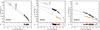 |
Fig. 1 Rest-frame γ-ray (grey), X-ray (black) and optical (orange) luminosity. The red triangle shows the value of average isotropic γ-ray luminosity Liso. Blue and green dotted lines represent the light curve best fit for the X-ray and optical bands, respectively. The complete version of the figure is available in Appendix A. |
3. Results
In Fig. .1, we show the γ-ray, X-ray, and optical rest-frame luminosity for all the GRBs with redshift of the complete sample. For each event we retrieved data in the γ-ray and in the X-ray bands from the online Swift Burst Analyser (Evans et al. 2010); Swift-BAT data have been rescaled to the Swift-XRT [0.3−10] keV energy range. The optical data were collected from all the available sources (published dedicated papers and/or GCNs). We then converted all the observed γ-ray and X-ray data into rest-frame luminosity in the [2−10] keV energy range (LBAT and LXRT) and optical data into rest-frame luminosity in the U-band (LOpt). For the optical conversion we considered the spectral and absorption parameters of each single burst from the detailed analysis of Covino et al. (2013) (see next section). The results of the light curves fitting in the X-ray and optical bands are reported in Tables 2 and 3, respectively.
In the X-ray band, 20% of the luminosity light curves are represented by a single power-law decay (class 0), 42% by a single break light curve (~36% from shallow to steep, class Ia, and ~6% from steep to shallow decays, class Ib), and the remaining 38% by a double break light curve (~36% by the canonical steep-shallow-steep decay, class IIa, and ~2% by the shallow-steep-shallow decay, class IIb). In the optical band, the behaviour is different, with the majority of the events (49%) belonging to class 0; 31% are described by a single break light curve (~24% of class Ia and ~7% of class Ib), 6% by the canonical double break light curve (class IIa), and the remaining 14% (8 out of 55) have no optical data available to assess their light curve behaviour.
Number of GRBs per light curve type.
3.1. Rest-frame optical luminosity
The majority of the optical observations for the GRBs in the sample were carried out in the optical R and I bands. Since the median redshift of our complete GRBs sample is z ~ 1.6 (Salvaterra et al. 2012), these observational bands would correspond to a rest-frame frequency νRF ~ 0.9 × 10¹⁵ Hz. This value is close to the U-band rest-frame frequency (νRF ≈ νU = 0.82 × 10¹⁵ Hz). After considering the spectral (βO) and rest-frame absorption (AV) parameters (Covino et al. 2013), we therefore reported the observed optical/IR flux of each burst to the correspondent rest-frame flux at the frequency νU and then converted it into rest-frame luminosity2 (Lopt, shown in Fig. .1).
In general, if a GRB is mainly observed in the optical band νobs, then the Galactic corrected observed flux (fobs) is reported to the rest-frame optical luminosity (Lopt) at the frequency νU by applying the formula ![Mathematical equation: \begin{eqnarray} L_{\rm opt} = 4 \pi d_{L}^{2} \times 10^{0.4A_{U}} \times f_{\rm obs} \times \left[\frac{\nu_{U}}{(1+{\it z}) \nu_{\rm obs}} \right]^{-\beta_{\rm O}} , \end{eqnarray}](/articles/aa/full_html/2014/05/aa23361-13/aa23361-13-eq32.png) (1)where 100.4AU is the absorption correction, dL is the luminosity distance, and z is the redshift of the GRB.
(1)where 100.4AU is the absorption correction, dL is the luminosity distance, and z is the redshift of the GRB.
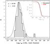 |
Fig. 2 Optical rest-frame luminosity (R-band, erg s-1 Hz-1) distribution at tRF = 12 h. The mean value of the distribution is μ = 29.9 with a dispersion σ = 0.8. Inset: cumulative distribution of the optical rest-frame luminosity for the BAT6 sample (red) and for a simulated population of GRBs obtained with the PSYCHE code (Ghirlanda et al. 2013). |
The result for each single burst is reported in one single panel of Fig. .1, where the optical behaviour is compared to the rest-frame luminosity in γ and X-rays. In Fig. 2 we show the R-band rest-frame optical luminosity, as estimated from Eq. (1) for the GRBs in our sample, which evaluated at trf = 12 h in the rest-frame. Considering the median redshift of the BAT6 sample with that choice, we considere a time in the observer frame larger than 1 day after the burst event. At such late times, the observed optical luminosity should come only from one component, which is the afterglow. As can be seen in Fig. 2, the bimodality of the luminosity distribution at that time, as claimed in previous works (e.g., Liang & Zhang 2006; Nardini et al. 2006; Kann et al. 2006; Nardini et al. 2008), is not confirmed with our complete sample. There are no clear gaps in the luminosity range 28 ≤ Log (LR) ≤ 30. Only one event has an extremely bright optical luminosity; this event correspond to GRB 070306, the event with the highest rest-frame optical absorption also found by Covino et al. (2013). The mean value of the LR distribution is μ = 29.96 (σ = 0.80) erg s-1 Hz-1. Assuming a central value for the R-band of νR = 4.6 × 10¹⁴ Hz, the mean value of the LR distribution of the BAT6 sample corresponds to μ = 44.6 erg s-1, which is consistent with the value found in other works (μ = 44.20, σ = 0.67 by Melandri et al. 2008; μ = 44.50, σ = 0.74 by Zaninoni et al. 2013).
The overall distribution of the Lopt for our complete sample (Fig. .1, second to last panel) spans ~4 orders of magnitude from a very early time up to days after the burst event. This trend is also mimicked by the distribution of the Eiso-normalised optical luminosity, which are the luminosities normalised to their isotropic energies (Fig. .1, last panel) where the dispersion at late times is even larger. In particular, no strong clustering at an early time is found for Lopt/Eiso and the scatter of the distribution remains nearly constant for the entire duration of the optical observation. This is in contrast to what was found by D’Avanzo et al. (2012) where the distribution of LX was strongly correlated with the isotropic energy. In Fig. 3, a direct comparison between the distributions of Eiso, LXRT, and Lopt of the BAT6 sample is shown: in that figure, we considere all the events with confirmed redshift for which the estimate of one of the three variables has been possible. In Fig. 4, we show how the Eiso-normalised optical luminosity (LR/Eiso; bottom panel) has a larger distribution with respect to the Eiso-normalised X-ray luminosity (LX/Eiso; top panel) as already described in D’Avanzo et al. (2012). This result strengthens the idea that the X-ray luminosity is a better proxy of the prompt emission, while the optical luminosity describes more accurately the afterglow emission.
The agreement between the γ-ray (LBAT) and X-ray (LXRT) light curves is quite good, where the latter typically seem to be a natural continuation of the former when there is still some overlap in time (i.e. for trf< 102 s). Coupled with the result that the light curves seem to have different behaviours in the X-ray and in the optical bands for the majority of the GRBs, this might indicate that the emission in the X-ray is still contaminated by the prompt emission of the GRB at least at very early times, while afterglow emission dominates in all bands (i.e., Ghisellini et al. 2009) at later times. For some cases, the back extrapolation of LXRT seems to under estimate (i.e., GRB 050416A and GRB 071117) or over estimate (i.e., GRB 061121) the LBAT. This might be only a visual effect for these events: there is a gap between the last emission detected in γ-ray (sometimes, the emission in γ-ray does not last more than few tenth of seconds) and the first detection in X-ray (sometimes, the observation in X-ray does not start before few hundreds of seconds).
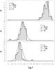 |
Fig. 3 Distributions of Eiso (top), LXRT (mid), and Lopt (bottom) of the BAT6 sample for all the events with a confirmed redshift. For each histogram, we report the number of events considered (#), the mean value (μ), and dispersion (σ) of the distribution. Units on the x-axis from top to bottom are erg, erg s-1 and erg s-1, respectively. |
 |
Fig. 4 Eiso-normalised LXRT (top) and Lopt (bottom). The latter has a larger dispersion than the former. |
3.2. Cumulative distribution
In the inset of Fig. 2, we compare the cumulative distribution of the observed optical luminosity for the BAT6 sample to the simulated cumulative distribution obtained with the PSYCHE code (Ghirlanda et al. 2013). This code generates a synthetic population of GRBs that reproduces some properties of the real population of GRBs observed by Swift, Fermi, and BATSE (e.g., flux and fluence distributions, rate of detected events and rest-frame Ep − Eiso correlation). Then, it calculates the flux (luminosity) at any given time and frequency. Therefore, starting from the observed properties of the BAT6 sample, we estimated the expected optical luminosity at tRF = 12 h. As it can be seen in Fig. 2 (inset), the simulated cumulative distribution (black solid line) agrees very well with the luminosity distribution observed for the BAT6 sample (red dashed line). The PSYCHE code is used here to compare the distribution of the simulated burst optical fluxes with the real ones. The comparison of the X-ray flux distribution is beyond the scope of the present paper and is included in a forthcoming dedicated paper.
The properties of the BAT6 sample can be reproduced by fixing the index of the expected power-law electron energy distribution p = 2.5, the ratio between the energy of non-thermal electrons and the energy dissipated at the shock ϵe = 0.02, the ratio between the energy gained by the magnetic field and the energy dissipated at the shock ϵB = 0.008, and the assumption that the parameter describing the density of the medium (n) has a uniform distribution between 0.1 and 30 cm-3 (Ghirlanda et al. 2013).
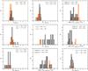 |
Fig. 5 Statistics of the decay indices and break times of the X-ray (black histograms) and optical (orange histograms) light curves for classes 0, Ia, and IIa present in the complete BAT6 sample. We do not display classes Ib and IIb, since the count is less than 5 events each. In each single panel, we also report the average and the standard deviation for the plotted parameters; break times (tb1 and tb2) are of order of 103 s (as reported in Tables 2 and 3). |
3.3. Statistics
The comparison of the rest-frame decay indices and the break times for the different classes in the X-ray and optical bands is shown in Fig. 5. We can observe few peculiarities:
-
For class 0 (single power-law), the average decay index of the X-ray light curves is steeper than the decay of the optical one. However, the two distributions are still consistent within the errors.
-
The distributions of the decay indices of the class Ia (single broken power-law) are in good agreement for the two bands (both α1,X,Ia ≃ α1,O,Ia and α2,X,Ia ≃ α2,O,Ia); however, the change of slope happens at later times in the optical band with respect to the X-ray band (tb1,O,Ia≫tb1,X,Ia).
-
For the class IIa (double broken power-law) the initial decay is always steeper in the X-ray (α1,X,IIa ≫ α1,O,IIa) and the change of slope from steep-to-shallow happens earlier in that band, which is ~1 order of magnitude in time (tb1,X,IIa ≪ tb1,O,IIa).
-
The flat phase of the class IIa (plateau) is similar for the two bands (α2,X,IIa ≃ α2,O,IIa).
-
The late decay indices and break times for the class IIa agrees within the errors (α3,X,IIa ≃ α3,O,IIa) while, the shallow-to-steep change of the slope in the optical band happens at later times (tb2,X,IIa ≪ tb2,O,IIa).
Although we do not show the histograms for class Ib in Fig. 5, the decay indices (pre- and post-break) in the X-ray band for class Ib are steeper than the ones observed in the optical band (α1,X,Ib ≫ α1,O,Ib and α2,X,Ib ≫ α2,O,Ib), while the break time in the two bands are similar (tb1,O,Ib ≃ tb1,X,Ib). The case of class IIb is seen only for one event in the X-rays (GRB 090926B), while class III, which is defined in Margutti et al. (2013), is never seen in our complete sample. The optical light curve displays a clear peak at early times for ~20% of the event in the BAT6 sample.
3.4. X-ray-optical comparison
The comparison between the light curves revealed that the classification is the same in the two bands (larger than what found by Zaninoni et al. 2013) for only 27% of the cases. The power-law decay for the majority of those events are consistent between the two bands, and the decay indices agrees even more when fewer breaks in the light curves are observed. This is an indication of a possible common (and unique) origin for the observed emission at these wavelengths for these events. For the remaining (large) fraction of GRBs in the BAT6 sample the behaviour is more complex and the agreement between the two bands is more difficult. Those are the cases where additional components (e.g., tail of the prompt emission, flares, and energy injection) are seen superposed with late time afterglow emission. This is a strong indication of different emitting regions that contribute in shaping the observed light curves. Similar contribution of these components for long periods is the cause of the complex behaviours observed when comparing X-ray and optical light curves (Ghisellini et al. 2009).
4. Conclusions
We investigated the rest-frame optical properties of the complete BAT6 sample. We unarguably demonstrated that the optical luminosity at trf = 12 h has a uniform distribution around a mean value Log(LR) = 29.9 (dispersion σ = 0.8). No bimodality is observed, as found in the published studies based on incomplete samples. Previous claims of bimodality were based on the inhomogenity of the analysis in determining the main parameters that influence the estimate of the rest-frame luminosity (βO and AV). In this work we used spectral and absorption parameters that has been estimated following a consistent procedure (described in details in Covino et al. 2013), and therefore, our result is more robust.
First of all, the comparison between optical and X-ray rest-frame light curves revealed that the complexity and different behaviours observed in these bands are strongly related to the emission components that might still be relevant in both bands. The observed light curves show similar decay slopes in the same time interval only for a few cases: this indicates a common origin of emission. Instead, this is not the case for the majority of the events of the sample (~70%), and the X-ray emission seems to still have a strong contribution from the prompt emission or from some late time central engine activity, whose contribution is negligible (or not detected) in the optical band where the afterglow emission dominates. Second, the distribution of the rest-frame X-ray luminosity is slightly broader (and naturally brighter) with respect to the distribution of the rest-frame optical luminosity, even though this trend is the opposite when considering the Eiso-normalised quantities. This again indicates that the emission in the X-ray is a better proxy of the prompt emission (since there is a long-lasting contribution of prompt emission in the X-ray), while the emission in the optical is strongly related only to the afterglow emission.
Online material
5. Complete version of Fig. 1
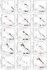 |
Fig. .1 Rest-frame γ-ray (grey), X-ray (black) and optical (orange) luminosity. The red triangle shows the value of average isotropic γ-ray luminosity Liso. Blue and green dotted lines represent the light curve best fit for the X-ray and optical bands, respectively. In addition: the last two panels are the rest-frame optical luminosity of the whole sample and the rest-frame optical luminosity, which are normalised by the isotropic energy (Eiso). The solid vertical line correspond to tRF = 12 h. |
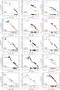 |
Fig. A.1 continued. |
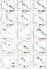 |
Fig. A.1 continued. |
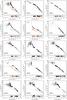 |
Fig. A.1 continued. |
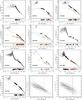 |
Fig. A.1 continued. |
We considered powerful and fast re-brightenings superposed to the normal decay at early times as flares, while bumps are broader features happening at later times.
For GRB 071117, we assumed βO = 1.0, since it was not possible to better constrain the spectral index due to the paucity of optical data.
Acknowledgments
We thank the anonymous referee for the valuable comments, which significantly contributed to improve the quality of the publication. This research has been supported by ASI grant INAF I/004/11/1. This work made use of data supplied by the UK Swift Science Data Centre at the University of Leicester.
References
- Campana, S., Salvaterra, R., Melandri, A. et al. 2012, MNRAS, 421, 1697 [NASA ADS] [CrossRef] [Google Scholar]
- Covino, S., Melandri, A., Salvaterra, R., et al. 2013, MNRAS, 432, 1231 [NASA ADS] [CrossRef] [Google Scholar]
- D’Avanzo, P., Salvaterra, R., Sbarufatti, B., et al. 2012, MNRAS, 425, 506 [NASA ADS] [CrossRef] [Google Scholar]
- Evans, P., Beardmore, A. P., Page, K. L., et al. 2009, MNRAS, 397, 1177 [NASA ADS] [CrossRef] [Google Scholar]
- Evans, P., Willingale, R., Osborne, J. P., et al. 2010, A&A, 519, A102 [NASA ADS] [CrossRef] [EDP Sciences] [Google Scholar]
- Gehrels, N., Chincarini, G., Giommi, P., et al. 2004, ApJ, 611, 1005 [NASA ADS] [CrossRef] [Google Scholar]
- Gehrels, N., Barthelmy, S. D., Burrows, D. N., et al. 2008, ApJ, 689, 1161 [NASA ADS] [CrossRef] [Google Scholar]
- Ghirlanda, G., Ghisellini, G., Nava, L., et al. 2012, MNRAS, 422, 2553 [NASA ADS] [CrossRef] [Google Scholar]
- Ghirlanda, G., Salvaterra, R., Burlon, D., et al. 2013, MNRAS, 435, 2543 [NASA ADS] [CrossRef] [Google Scholar]
- Ghisellini, G., Nardini, M., Ghirlanda, G., & Celotti, A. 2009, MNRAS, 393, 253 [NASA ADS] [CrossRef] [Google Scholar]
- Kann, D. A., Klose, S., & Zeh, A. 2006, ApJ, 641, 993 [NASA ADS] [CrossRef] [Google Scholar]
- Kann, D. A., Klose, S., Zhang, B., et al. 2011, ApJ, 734, 96 [NASA ADS] [CrossRef] [Google Scholar]
- Li, L., Liang, E.-W., Tang, Q.-W., et al. 2012, ApJ, 758, 27 [NASA ADS] [CrossRef] [Google Scholar]
- Liang, E., & Zhang, B. 2006, ApJ, 638, 67 [Google Scholar]
- Liang, E.-W., Li, L., Gao, H., et al. 2012, ApJ, 774, 13 [Google Scholar]
- Mangano, V., Holland, S. T., Malesani, D., et al. 2006, A&A, 470, 105 [Google Scholar]
- Margutti, R., Zaninoni, E., Bernardini, M. G., et al. 2013, MNRAS, 428, 729 [NASA ADS] [CrossRef] [Google Scholar]
- Melandri, A., Mundell, C. G., Kobayashi, S., et al. 2008, ApJ, 686, 1209 [NASA ADS] [CrossRef] [Google Scholar]
- Melandri, A., Sbarufatti, B., D’Avanzo, P., et al. 2012, MNRAS, 421, 1265 [NASA ADS] [CrossRef] [Google Scholar]
- Nardini, M., Ghisellini, G., Ghirlanda, G., et al. 2006, A&A, 451, 821 [NASA ADS] [CrossRef] [EDP Sciences] [Google Scholar]
- Nardini, M., Ghisellini, G., & Ghirlanda, G. 2008, MNRAS, 386, 87 [Google Scholar]
- Nava, L., Salvaterra, R., Ghirlanda, G., et al. 2012, MNRAS, 421, 1256 [NASA ADS] [CrossRef] [MathSciNet] [Google Scholar]
- Nousek, J. A., Kouveliotou, C., Grupe, D., et al. 2006, ApJ, 642, 389 [NASA ADS] [CrossRef] [Google Scholar]
- Nysewander, M., Fruchter, A. S., & Peer, A. 2009, ApJ, 701, 824 [NASA ADS] [CrossRef] [Google Scholar]
- Oates, S. R., Page, M. J., Schady, P., et al. 2009, MNRAS, 395, 490 [NASA ADS] [CrossRef] [Google Scholar]
- Roming, P. W. A., Koch, T. S., Oates, S. R., et al. 2009, ApJ, 690, 163 [NASA ADS] [CrossRef] [Google Scholar]
- Rykoff, E. S., Aharonian, F., Akerlof, C. W., et al. 2009, ApJ, 702, 489 [NASA ADS] [CrossRef] [Google Scholar]
- Salvaterra, R., Campana, S., Vergani, S. D., et al. 2012, ApJ, 749, 68 [NASA ADS] [CrossRef] [Google Scholar]
- Zaninoni, E., Bernardini, M. G., Margutti, R., Oates, S., & Chincarini, G. 2013, A&A, 557, A12 [NASA ADS] [CrossRef] [EDP Sciences] [Google Scholar]
- Zhang, B., Fan, Y. Z., Dyks, J., et al. 2006, ApJ, 642, 354 [NASA ADS] [CrossRef] [Google Scholar]
All Tables
All Figures
|
Fig. 1 Rest-frame γ-ray (grey), X-ray (black) and optical (orange) luminosity. The red triangle shows the value of average isotropic γ-ray luminosity Liso. Blue and green dotted lines represent the light curve best fit for the X-ray and optical bands, respectively. The complete version of the figure is available in Appendix A. |
| In the text | |
|
Fig. 2 Optical rest-frame luminosity (R-band, erg s-1 Hz-1) distribution at tRF = 12 h. The mean value of the distribution is μ = 29.9 with a dispersion σ = 0.8. Inset: cumulative distribution of the optical rest-frame luminosity for the BAT6 sample (red) and for a simulated population of GRBs obtained with the PSYCHE code (Ghirlanda et al. 2013). |
| In the text | |
|
Fig. 3 Distributions of Eiso (top), LXRT (mid), and Lopt (bottom) of the BAT6 sample for all the events with a confirmed redshift. For each histogram, we report the number of events considered (#), the mean value (μ), and dispersion (σ) of the distribution. Units on the x-axis from top to bottom are erg, erg s-1 and erg s-1, respectively. |
| In the text | |
|
Fig. 4 Eiso-normalised LXRT (top) and Lopt (bottom). The latter has a larger dispersion than the former. |
| In the text | |
|
Fig. 5 Statistics of the decay indices and break times of the X-ray (black histograms) and optical (orange histograms) light curves for classes 0, Ia, and IIa present in the complete BAT6 sample. We do not display classes Ib and IIb, since the count is less than 5 events each. In each single panel, we also report the average and the standard deviation for the plotted parameters; break times (tb1 and tb2) are of order of 103 s (as reported in Tables 2 and 3). |
| In the text | |
|
Fig. .1 Rest-frame γ-ray (grey), X-ray (black) and optical (orange) luminosity. The red triangle shows the value of average isotropic γ-ray luminosity Liso. Blue and green dotted lines represent the light curve best fit for the X-ray and optical bands, respectively. In addition: the last two panels are the rest-frame optical luminosity of the whole sample and the rest-frame optical luminosity, which are normalised by the isotropic energy (Eiso). The solid vertical line correspond to tRF = 12 h. |
| In the text | |
|
Fig. A.1 continued. |
| In the text | |
|
Fig. A.1 continued. |
| In the text | |
|
Fig. A.1 continued. |
| In the text | |
|
Fig. A.1 continued. |
| In the text | |
Current usage metrics show cumulative count of Article Views (full-text article views including HTML views, PDF and ePub downloads, according to the available data) and Abstracts Views on Vision4Press platform.
Data correspond to usage on the plateform after 2015. The current usage metrics is available 48-96 hours after online publication and is updated daily on week days.
Initial download of the metrics may take a while.