| Issue |
A&A
Volume 565, May 2014
|
|
|---|---|---|
| Article Number | A41 | |
| Number of page(s) | 8 | |
| Section | Interstellar and circumstellar matter | |
| DOI | https://doi.org/10.1051/0004-6361/201323216 | |
| Published online | 01 May 2014 | |
On the decades-long stability of the interstellar wind through the solar system
1 GEPI, Observatoire de Paris, CNRS, Université Paris Diderot, Place Jules Janssen, 92190 Meudon, France
e-mail: This email address is being protected from spambots. You need JavaScript enabled to view it.
2 LATMOS, Université de Versailles Saint Quentin, INSU/CNRS, 11 Bd D’ Alembert, 78200 Guyancourt, France
Received: 8 December 2013
Accepted: 30 January 2014
Abstract
We have revisited the series of observations recently used to infer a temporal variation in the interstellar helium flow over the past forty years. Concerning the recent IBEX-Lo direct detection of helium neutrals, there are two types of precise and unambiguous measurements that do not rely on the exact response of the instrument: the count rate maxima as a function of the spin angle, which determines the ecliptic latitude of the flow, and the count rate maxima as a function of IBEX longitude, which determines a tight relationship between the ecliptic longitude of the flow and its velocity far from the Sun. These measurements provide parameters (and couples of parameters in the second case) that are remarkably similar to the canonical, old values. In contrast, the preferred choice of a lower velocity and higher longitude reported before from IBEX data is only based on the count rate variation (at each spin phase maximum) as a function of the satellite longitude, when drifting across the region of high fluxes. We have examined the consequences of dead-time counting effects and conclude that including them at a realistic level is sufficient to reconcile the data with the old parameters, calling for further investigations. We discuss the analyses of the STEREO pickup ion data and argue that the statistical method that has been preferred to infer the neutral flow longitude (instead of the more direct method based on the pickup ion maximum flux directions) is not appropriate. Moreover, transport effects may have been significant at the very weak solar activity level of 2007−2009, in which case the longitudes of the pickup ion maxima are only upper limits on the flow longitude. Finally, we found that using some flow longitude determinations based on UV glow data is not adequate. Based on this global study, and at variance with recent conclusions, we find no evidence for a temporal variability of the interstellar helium flow. This has implications for inner and outer heliosphere studies.
Key words: interplanetary medium / Sun: heliosphere / solar wind / Sun: UV radiation / ISM: general / solar neighborhood
© ESO, 2014
1. Introduction
The low-energy, neutral helium flow measured in the solar system has its origin in the ≃25 km s-1 relative motion of the Sun with respect to the ambient interstellar cloud. Interstellar helium measurements are crucial because, at variance with hydrogen, helium atoms experience very little charge exchange with the solar wind ions, and as a consequence, the helium flow velocity vector is the best indicator of the actual relative motion. The precise direction of the helium flow also serves as a reference for measuring other species, and inferred differences can be used to derive the detailed coupling between the interstellar and solar plasmas (e.g., Izmodenov et al. 1999; Lallement et al. 2005). Possessing a very accurate value of the interstellar flow parameters is also particularly timely, because the two Voyager spacecraft are currently producing new and exciting data on the structure of the inner and outer heliosheath, including the recent crossing of the heliopause by Voyager 1 (Gurnett et al. 2013; Stone et al. 2013; Krimigis et al. 2013).
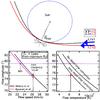 |
Fig. 1 Interplay between the flow parameters: Top: an extremely solid measurement of IBEX-Lo is the Earth longitude of the maximum neutral atom flux λE, where the entrance field (hatched cones) is directed against the flow (≃ortho-radial bulk flow). Each value of λE corresponds to a continuum of pairs of flow longitude and speed values, as illustrated by the two (black and red) trajectories. Bottom left: the corresponding longitude-speed relationship inferred by Möbius et al. (2012) (black line) and based on the measurement of λE with IBEX-Lo. Also shown is the central part of the chi-square parametric image of Bzowski et al. (2012), which also corresponds to the same longitude-speed link. The consensus pair of values is fully compatible with those relationships. Bottom right: the temperature-longitude derived by Möbius et al. (2012) based on the flux measurements during the rotation around the IBEX spin axis. The authors considered both the absence (top curve) and the presence (bottom curve) of high rate suppression of events (or dead-time). The consensus temperature of ≃6300 K is compatible with the consensus flow longitude of ≃75.4° for a dead-time on the order of 5 ms or slightly higher, i.e., realistic values according to Möbius et al. (2012). |
After the pioneering measurements of the HeI 58.4nm solar backscattered radiation (Weller & Meier 1974; Ajello 1978; Ajello et al. 1979; Weller & Meier 1979, 1981), the first in situ measurements of interstellar helium were obtained, starting with pickup ions (Möbius et al. 1985, 1995), followed by direct neutral helium atom detection (Witte et al. 1993). Extensive efforts were done in 2003−2004 (ISSI workshop) to analyze all available datasets in a synthesized manner. In particular, the new analyses resolved the remaining strong discrepancies between flow temperature and velocities that were independently derived from UV and particle data (Lallement et al. 2004a,b; Vallerga et al. 2004). A canonical set of parameters (flow direction, flow speed and temperature) was presented by Möbius et al. (2004) based on a synthesis of all data. Those flow parameters are very close to the parameters of Witte (2004) derived from the Ulysses atom detection data.
More recently, the Interstellar Boundary EXplorer (IBEX) mission has produced unprecedented measurements of neutral atoms in the heliosphere, in particular energetic atoms generated in the outer heliosphere (McComas et al. 2009), as well as low energy atoms of direct interstellar origin, especially helium atoms (Hłond et al. 2012). The analysis of the first two years of IBEX-Lo helium data (2009−2010) led to the derivation of helium flow parameters that are quite different from the canonical values, in particular a flow longitude of 79.2°, instead of 75.4°, and a speed of 22.8 km s-1 instead of 26.3±0.5 km s-1 (Bzowski et al. 2012; Möbius et al. 2012). Soon after those new parameters were published, Drews et al. (2012) announced similar values of the flow longitude, based on their analysis of pickup ions (PUIs) detected by STEREO/PLASTIC.
The value of the flow velocity has a strong influence on the heliospheric interface structure, and indeed the IBEX-Lo low speed was used as an argument to dismiss the existence of an interstellar bow-shock ahead of the heliopause (McComas et al. 2012). It also motivated new theoretical studies about the actual nature of the outer heliosheath (Zank et al. 2013; Zieger et al. 2013). A compilation of all results obtained since the 70s and including the new IBEX-Lo and STEREO determinations has been interpreted as a statistically significant demonstration of a temporal change in the longitude of the interstellar helium flow velocity vector over the past decades (Frisch et al. 2013), which is very surprising owing to the wide mean free paths against collisions in low density clouds such as the circumsolar one.
In this work we revisit the most recent datasets on the helium flow and their interpretations. Section 2 is devoted to the IBEX-Lo results that have a very strong statistical weight in the analysis of the longitude temporal variation, thanks to the accuracy of the measurements. In Sect. 3 we discuss the PUIs and backscattered radiation measurements. Section 4 synthesizes the data and most reliable parameters and discusses the likelihood of temporal variations of the flow over the past decades.
2. Helium flow parameters from IBEX-Lo in situ data
With the IBEX satellite long-duration direct measurements of helium atoms have for the first time been and are currently being made from the Earth orbit (McComas 2012; Hłond et al. 2012) in the keV energy range with IBEX-Hi (Funsten et al. 2009) and at lower energy with IBEX-Lo (Fuselier et al. 2009). Because gravitational effects and ionization by the solar radiation and solar particles have very strong impacts on the low-energy interstellar flow within a few AU, IBEX-Lo data are analyzed by comparison with models that follow the flow and take all those effects into account. Bzowski et al. (2012), Möbius et al. (2012), and Lee et al. (2012) have developed appropriate, extensive analytical and numerical models supporting the analysis of the neutral helium data recorded since 2009. Bzowski et al. (2012) derived a set of parameters for the helium flow from the numerical analysis of the first two years of data, in rough agreement with the more analytical determinations by Möbius et al. (2012).
There are two puzzling coincidences in the new IBEX-Lo helium parameters that have not been discussed and that deserve more attention. First, the pair of new flow longitude λ and velocity V values (at infinity) corresponds to a location of maximum count rate along the Earth orbit that is remarkably similar to the location one would find for the old parameters. This is important because an extremely solid and precise measurement of IBEX-Lo is indeed this Earth longitude of maximum count rate, which corresponds to the strongest flux of neutral atoms entering the IBEX-Lo field-of-view (FOV). This happens where the boresight axis is directed against the flow. Since this axis is close to perpendicular to the Sun-Earth direction, this implies a helium flow that is close to tangential to the Earth motion or an ortho-radial bulk flow at 1 AU. It is well known, however, that there is a continuum of flow longitude and speed pairs that corresponds to the same unique value of Earth longitude λE with such an orthoradial flow orientation, as illustrated by Fig. 1. The lower the flow speed at large distance from the Sun, the stronger the curvature of the trajectories due to the solar gravitational field, an effect that tends to increase λE if the distant flow longitude remains the same, but can be compensated for by an increase in the flow longitude that has the effect of rotating the whole set of trajectories around the Sun along an ecliptic polar axis. This longitude-speed relationship has been calculated analytically by Möbius et al. (2012) and is independently found numerically by Bzowski et al. (2012) as the locus of minimum χ2 in the V-λ space. Both (and very similar) relationships, taken from their respective publications and based on the precise measurement of λE with IBEX-Lo, are displayed together in Fig. 1. It can be seen from the figure how the pair of old values is quite compatible with this relationship. It implies that, if indeed the flow has rotated by about four degrees with respect to its former direction, its speed has coincidentally varied by the exact amount that is needed to keep the same Earth location of tangential flow. Because the IS flow change is a phenomenon in the interstellar (IS) medium that is not related to the Earth orbit, this coincidence alone is suspicious.
The second coincidence is the total absence of change of the flow ecliptic latitude β. While λ has varied by about four degrees, no variation in β is detected remarkably, despite uncertainties on the latitude measurements that are far smaller (on the order of 0.2°) than the uncertainties on the longitude. Interestingly, another extremely solid measurement by IBEX-Lo is indeed this latitude β, accurately measured by the spin phase of the maximum count rate during the rotation of IBEX around an axis near the direction of the Sun. As a matter of fact, the latitude of this maximum count location changes very little under the effect of gravitation and Earth location. Here, again, the orientation of the ecliptic plane and the interstellar medium’s spatial variations are unrelated, and simultaneous changes of both the flow longitude and latitude are more likely than the change of only one of the two. We emphasize again that these two coincidences correspond to unambiguous measurements based only on MAXIMA of the count rate. In both cases the measured quantities, namely the parameter β and the combination of the two other parameters λ and V, correspond exactly to the previous consensus values. Given these coincidences, it is important to understand what is influencing the derivation of the new pair of parameters (79.2°, 22.8 km s-1) that emerges out from the works quoted above and what dismisses the old pair (75.4°, 26.3 km s-1), knowing that they both correspond to the same Earth longitude for maximum rate. Since we fully trust the models carefully developed and cross-checked by Lee et al. (2012), Möbius et al. (2012) and Bzowski et al. (2012), a search should be oriented toward potential biases. Indeed, the existence of a bias is suspected, owing to the puzzling iso-χ2 curves presented by Bzowski et al. (2012), which display two unexplained maxima.
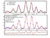 |
Fig. 2 Top: concatenated data and model values taken from Bzowski et al. (2012) for orbits 13 to 20 in year 2009. Both data and model have been precisely computed by the authors for the same geometry and the same time intervals. The abscissa represents the data point number, and both data and models are the normalized values of Bzowski et al. (2012). The Witte et al. model decreases more rapidly than the count rate for Earth ecliptic longitudes that are both lower and higher than the maximum flux longitude λE. Middle: example of scaling of the Witte et al. model to the count rates assuming a dead-time of 7 ms, a maximum count rate of 25.8 counts/s due to He atoms and an electron background of 22 counts/s. Units are counts/s. The sum of squared residuals after normalization is slightly higher than for the Bzowski et al. (2012) parameters (see text) but there is no model parameter adjustment here, unlike in their work. Similar residuals can be obtained for realistic ranges of the three above parameters. Bottom: a small asymmetry is found in all residuals, that we attribute to the fact that the Witte et al longitude is slightly too high compared to the actual flow longitude. A lower longitude should significantly improve the data-model agreement. New studies taking the dead-time into account should allow to obtain very accurate flow parameters. |
For the study we describe below, we have made extensive use of the count rates and the model results presented by Bzowski et al. (2012) in their Fig. 18, which is devoted to the year 2009. We have extracted the normalized, orbit-integrated data computed in spin angle sectors from the figure, as well as the two old and new model values adapted to the same observing geometry and instrument characteristics. We concatenated those values to obtain a single series of data for all orbits of interest and corresponding series of model values. Figure 2 shows the concatenated data and the corresponding models, and clearly reveals the trends for the two different models. The new model count rates follow the data in a much better way, essentially because the rates decrease in the same way as the data as a function of the observer longitude (or orbit number) on both sides of the maximum flux location (the tangential flow location described above). In contrast, the old model rates decrease more rapidly than the measurements as the longitude difference increases. The physical reason for a greater or smaller decrease in the fluxes when moving away from the maximum flux location (valid for measurements made tangentially to the Earth orbit) is the following: the closer the curvature of the observer’s orbit (here the Earth orbit) and the curvature of the average He trajectory, the slower the decrease in the entrance atom flux, because the observer motion accompanies the helium atom motion better (see Fig. 1 top). Because most He trajectories in this sidewind location (around longitudes on the order of 130°) are less bent than the Earth orbit, a slower decrease happens for a lower speed of the atoms at infinity, since their trajectories are more strongly bent at 1 AU. Looking at Fig. 2, it is clear that this is the dominant effect that favors the low speed found from the IBEX-Lo data (and subsequently the higher longitude, because they are very strongly linked) and disfavors the old values. However, this implies that this preference of the low speed is based entirely on count rate variations around the maximum. Any departure between the actual and the hypothesized response to the entrance neutral atom flux may influence the adjustment to the data. It is thus important to consider potential unaccounted-for biases in the sensitivity of the count rate to the atom fluxes, since they may influence the derivation of the longitude-speed pair. In what follows we consider the influence of non-linear response due to a suppression of events for high counting rates. This effect is very likely to be present and has been mentioned and partly studied by Möbius et al. (2012). Our goal is solely to investigate whether the flow parameters found by Witte et al. may be compatible with the data when accounting for nonlinearity. A full adjustment of parameters is far beyond the scope of this study.
Möbius et al. (2012) have documented the suppression of events due to high rate counting. Both the time to record an event by the detector and the time taken by the Central Electronic Unit (CEU) to analyze the event, construct histograms, and communicate with the spacecraft result in a loss of true events. We let NV and NTM be the number of events in a second of counting time of true events and events transmitted through telemetry, respectively. The number of events NTM sent to telemetry is lower than NV. This instrumental effect, which results in a nonlinearity of response, is thoroughly discussed in Möbius et al. (2012, Appendices A and B). It can be described in terms of a dead-time τD, during which the instrument cannot record a new event after the proper record of one event. It is well known that the value of NV can be retrieved from NTM if τD is known: 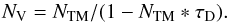 (1)It is clear from the formula that the larger NTM, the greater the loss of true events, measured by the factor NV/NTM. The events are triggered either by the detection of one He atom, or by some residual electrons forming a background with a true rate RBGV (Möbius et al. 2012). Therefore, NV = NHeV + RBGV and, similarly, NTM = NHec + RBGc are the sum of the two types of events, with the index He of helium atoms events, BG for electrons, V for true, and c for counted. Therefore, Eq. (1) may be transformed (to let appear explicitly the electron background) into
  (2)which may be decomposed into two formulae:
  (3)which is identical to formula (B1) of Möbius et al. (2012), and
  (4)Both the He counts and the background counts are reduced by the same ratio by the dead time effect. It must be kept in mind that, even if RBGV is constant, the observed background RBGc is not constant. The following numerical values are taken from Möbius et al. (2012). On average, IBEX-Lo counts RBGc = 22 electrons s-1. At its peak, the observed helium count rate reaches NHec ≃ 25.3 counts s-1. Möbius et al. (2012) indicate in their Appendix B that a dead time of up to 5 ms was derived from their analysis, but that this estimate is not very accurate, owing to the various assumptions made for its derivation. Introducing these values in the above equations, and noting that NHeV/NHec = RBGV/RBGc (both He atoms and electrons are reduced in the same proportion by the dead time effect), we find NHeV ≃ 1.31NHec. Interestingly, this ratio is close to the ratio between the old and new model values for the second and third orbits before and after the maximum count orbit, i.e. close to what differentiates the two models.
Möbius et al. (2012) have discussed this point, in the context of determining the temperature of helium by analyzing the variation in the He flow as a function of the spin phase (roll angle about the spin axis) when IBEX was near the maximum of helium detection. The authors explain in their Appendix B that if τD is not negligible, the relation between the observed and true rates is a function of the spin angle, and the observed angular distributions appear wider than the original distributions. If uncorrected, this would translate into derivation of an apparently higher temperature. Following these words of caution, Möbius et al. (2012) consider both the absence and presence of a high-rate suppression of events (or dead-time effect) in their determination of the flow temperature. Figure 1 shows one of their synthetic analytical results, namely the temperature-longitude relationships derived from the Earth longitude for maximum flux and both the maximum flux spin phase and flux peak angular width. It is interesting to see from the figure how the old longitude value of ≃75.4° compares with the old temperature value of ≃6300 K and the old speed 26.2 km s-1. Their compatibility requires a dead time slightly above the value of 5 ms, i.e., a value they consider as realistic. On the other hand, the new longitude value of ≃79.2° is compatible with a temperature of ≃6000 K and the new speed on the order of 23 km s-1 in the absence of a dead-time effect.
In their extensive comparison of IBEX-Lo data with sophisticated models of interstellar helium flow at 1 AU, Bzowski et al. (2012) have not taken the effect of dead-time into account in their numerical modeling of the first two years of data. This agrees with the compatibility between the longitude, temperature, and speed they have derived, which corresponds to the case of null dead-time, according to the Fig. 8 from Möbius et al. (2012). In view of these considerations, we have studied the modifications of the data-model agreement in the frame of dead-time existence, using the data and model values quoted by Bzowski et al. (2012). Our goal is to investigate whether dead-time effects may reconcile the flux decrease predicted by the old model with the data when moving away from the maximum flux location. The first argument is that neglecting these effects reduces the amplitude of the variations, as just explained. The second one is based on the background removal. If, as we assume, Bzowski et al. (2012) did not take the dead time into account, this implies they have subtracted a constant background rate of electrons from the observed count rates, a value that may be derived from the observed data when the helium flow is expected to be zero (i.e., when the spin angle is away from the helium flow). As we have shown above, in the presence of dead-time effects, removing a constant background is not applicable since the counted background RBGc is not constant and depends on the helium flow count rate, and since both effects conspire to decrease the contrast between high and low He rates when going from true values to observed values.
We have used a grid of three assumed parameters for our study: i.e., the dead time τD, the maximum measured value of the helium count rate  , the background value RBGc removed by Bzowski et al. (2012), a value chosen to ensure a decrease to zero of the observed rate far from the helium flow detection. We have varied those parameters within ranges that include the realistic values quoted by Möbius et al. (2012). The choice of τD and RBGc is imposing the true value of the background RBGV based on the formula (4) and NHec = 0. For each measurement in Fig. 2 that has been normalized at its maximum value over all orbits by Bzowski et al. (2012), we multiply this normalized value of the observed count rate by to represent the measured rate in counts/s, then add the measured background RBGc. This gives the measured rate before background removal. We then transform this rate into a true total rate NHeV + RBGV (which would have been observed without dead time effect) by using the formula (1). After subtraction of RBGV, we are left with the true He rate. We then normalize this true rate again and compute the quadratic sum of differences between this rate and the Witte et al. normalized model. We finally extract from the grid of results those displaying a good agreement between data and model, and for the most realistic parameters – i.e., dead time values on the order of 5 ms – maximum observed flux rates on the order of 25 counts s-1 and background on the order of 22 counts s-1. Since the methods used by Möbius et al. (2012) and Bzowski et al. (2012) differ and since we do not know the exact values of the removed background and maximum sector-average flux used in the latter work, we allow for a very small departure from these two parameters.
We show in Fig. 2 one example of our computations, chosen for its background and maximum count rate values that are very close to the values quoted by Möbius et al. (2012), and for a dead time of 7 ms, a value that is acceptable according to Fig. 1 (bottom). We have superimposed the true count rate and the scaled Witte et al. model values. We can compare the quality of this solution by comparing the data-model residuals with those derived from the new model values taken from Bzowski et al. (2012). The sum of squared residuals for this example is 0.0034 to be compared with 0.0031 (using the same normalization), demonstrating that such solutions should definitely be considered, especially considering that we did not perform any adjustment here of the model parameters and instead kept the Witte et al. model. Smaller residuals could certainly be found if a real adjustment of the model parameters were done. Indeed, the residuals show a small, but significant increase with the Earth longitude (Fig. 2 bottom). We believe that this trend demonstrates the need for a slightly lower longitude than the canonical one. We note that a longitude closer to 75° than 75.4° would be in very good agreement with a ≃7 ms dead time according to Fig. 8 in Möbius et al. (2012) (or Fig. 1 bottom). On the other hand, even this relative difference of 10% on the residuals is smaller than the distance from the primary to the secondary (unexplained) minimum of the χ2 found by Bzowski et al. (2012), if we use the variance around the primary minimum as a unit. The good agreement obtained between data and model, based on the Witte et al. parameters is a strong argument in favor of the relevance of those parameters, especially given the two extraordinary coincidences mentioned above, namely that the measurements that do not depend on the proportionality of the count rate to the incoming atom flux provide parameters (the latitude and the longitude-speed pair) in very good agreement with those canonical values. Again, a full adjustment of model parameters is beyond the scope of this study, since our focus is the temporal variation of the longitude. In this respect, we argue that it is premature to use the new longitude and velocity before the question of the dead time correction is fully settled. On the other hand, this first-order study shows that future additional IBEX-Lo data analysis should provide extremely precise measurements of the flow parameters.
3. Other data
3.1. Pickup-ions
Drews et al. (2012) have analyzed He+, O+, and Ne+ PUI flux measurements made by the PLAsma and SupraThermal Ion Composition instrument (PLASTIC) instrument on the Solar TErrestrial RElations Observatory mission (STEREO) between 2007 and 2010 (Galvin et al. 2008; Drews et al. 2010). The four orbits allow the He+ focusing cone to be detected four times and the Ne+ cone twice. There are also very broad and shallow flux enhancements (compared to the sidewind minima) approximately centered on the upwind direction called crescent maxima. The authors first show Gaussian fits to the average cones of He+ and Ne+ and the O+ crescent, superimposed on the measurements. Fluxes are averaged over the four orbits. They use a statistical method to estimate the error on the centers of those three features, instead of errors generated during the fitting procedure. The best-fit flow longitude values they quote are 75.0 ± 0.3°, 75.0 ± 2.9°, and 79.2 ± 1.4° for He+, Ne+, and O+, respectively. The first two values are in good agreement with the consensus longitude value. The third is out of the allowed range. In a second step of the analysis, they show a sophisticated, extensive statistical study of the whole dataset based on the assumptions that the flow direction has not changed over the four years of data and that the ionization of the neutral atoms responsible for the PUIs has varied very smoothly. As a consequence, the very strong fluctuations of the observed PUI fluxes can be decoupled from their creation and result only from the solar wind variability. The output of this study is a series of eleven values for the flow longitude derived from the eleven possible combinations of orbits. Based on this statistical study they derive weighted mean values of the flow longitude of 77.4 ± 1.9° and 80.4 ± 5.4° from the He cone and crescent, 77.4 ± 5.0° and 79.7 ± 2.6° from the Ne cone and crescent, and finally 78.9 ± 3.1° from the O+crescent.
The question we are addressing in this study is whether there is a temporal variability of the interstellar flow outside the heliosphere and which measurements can be used for this purpose. This includes (i) which type of method is likely to provide accurate values of the flow within the heliosphere; (ii) which species are appropriate for the derivation of the flow outside the heliosphere, (iii) whether PUI fluxes maxima are appropriate in general for the direction of the flow? Hereafter we consider these three points.
-
(i)
Although it is ingenious and able to provide estimates of errors, we have concerns about the method based on orbit combinations and the separation of temporal and spatial effects. The main concern is the assumption of a smoothly varying ionization. Drews et al. (2012) consider only the photoionization and omit the second source of ionization, electron impact. Theoretical calculations and observational studies of the neutral helium cone with UVCS on SOHO have demonstrated that electron impact can be responsible for a very large fraction of PUIs and, important here, especially in response to dense solar wind streams that possess large supra-thermal electron tails (Rucinski & Fahr 1989; Lallement et al. 2004b). According to the latter study, in stationary conditions and at 1 AU the fraction of PUIS born after electron impact may reach 30% of their total flux, both on the upwind and downwind sides, and this effect may explain temporarily observed correlations between H and He PUIs fluxes, as well as the anticorrelation between the wind speed and the He+ fluxes. This means that in nonstationary conditions there may be a very strong variability from one region to the other in response to solar streams, as well as local ratios between the two kinds of PUIs significantly above this value. This also implies that the assumed absence of coupling between the solar wind induced variability and their creation by ionization of neutrals is not a fulfilled condition. We also have other concerns about the assumption of eleven fully independent determinations, since the combinations or orbits are based on four orbits only, and thus the eleven realizations are not fully independent. As a conclusion, we believe that the direct Gaussian fits to actual data mentioned above provide more reliable values of the PUI flux maxima longitudes.
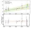
Fig. 3 Top: the original figure from Frisch et al. (2013) showing the inferred temporal increase of the helium wind longitude. Bottom: our revisited set of appropriate measurements. Filled circles are the data points we consider for linear fits. Longitudes derived from PUI data (augmented by 2σ) serve only as upper limits. Shown are the central, upper, and lower trends allowed by the fits. Stationarity is contained within the solutions. The question mark corresponds to the IBEX period and the Witte et al. longitude, not included in the fit (the IBEX-Lo result is also not included, according to Sect. 2). PUI data points are slightly displaced in the figure to avoid overlap.
-
(ii)
The use of oxygen ions for deriving the direction of the oxygen flow that enters the inner heliosphere is appropriate, but not for deriving the flow outside the heliosphere. As a matter of fact, as quoted by Drews et al. (2012), a deflection of the flow due to secondaries created by charge exchange is as likely as for hydrogen. Subsequently, the O+ crescent should not be used for the interstellar flow longitude study and should not be included in the Frisch et al. (2013) study.
-
(iii)
As mentioned by Drews et al. (2012), transport effects may be significant for PUIs. Chalov & Fahr (2006) have computed these effects and find potential deviations on the order of 5° on the He+ downwind cone at 1 AU. Interestingly, owing to the Parker spiral orientation, the PUIs maxima are always displaced towards HIGHER longitudes. The amplitude of the displacement depends on the level of turbulence, the SW characteristics, and the distance to the Sun. As a consequence, the average longitudes of the PUIs enhancements should be considered as UPPER LIMITS of the interstellar neutral flow longitude. Indeed, one very interesting result of Drews et al. (2012) is the systematic and strong discrepancy they find between the longitudes derived from the upwind and downwind data, which in principle should be identical. The authors mention the transport effects as the likely source of this discrepancy, reinforcing our argument that is not possible to use the PUI-derived longitudes in another manner than as upper limits. We suggest that the upwind deviations are likely to be stronger than for the focusing cones, since PUIs are created closer to the Sun on the upwind side (see, e.g. Fig. 11, of Lallement et al. 2004b), hence upwind PUIs collected at 1 AU. may have experienced stronger turbulence and more transport effects than the downwind PUIs. The Drews et al. (2012)crescent and cone discrepancies certainly deserve further study, with the transport effects taken into consideration. Important is that diffusion along the field lines may be much stronger in 2007−2010 at a time of very weak activity, than in the conditions prevailing in 2000 and experienced by the PUIs recorded by ACE (Gloeckler et al. 2004).
3.2. Solar backscatter radiation
Frisch et al. (2013) include in their analysis a flow direction corresponding to the Mariner 10 analysis (Ajello 1978; Ajello et al. 1979). We note however that the direction quoted in this work has been derived from H Lyα observations, namely from the downwind Lyα minimum; i.e., it applies to the neutral hydrogen and not to helium. In the early years of UV glow measurements, it had not been considered that the helium and hydrogen flows could enter the solar system from different directions, and the authors had adjusted models to the Mariner 10 He and H data for the same directional parameters. Since then measurements are much more precise and a difference could be established (Lallement et al. 2005). Indeed the longitude of the hydrogen flow has been found to be smaller by about ≃ 2 − 3° than the helium longitude. Consequently, it does not seem appropriate to use this direction in the context of the helium direction.
In their analysis Frisch et al. (2013) also include two distinct results based on the Prognoz satellite measurements of 58.4 nm backscattered radiation, a first longitude determination of 72.2° and a second one of 74.5°. The first lower value has some influence on their inferred positive slope for the evolution of the flow longitude. However, a careful look at the Dalaudier et al (1984) article shows clearly that the first value should definitely upper limits NOT be included. Dalaudier et al (1984) presented this first determination as a preliminary test based on angles roughly determined from a fraction of the scans. The goal of the test was to demonstrate that their Prognoz 30.4 nm dataset reveals well the helium cone, and it was included because this article is the first analysis of the data. They do not consider further this result, which is not even mentioned in the abstract or in the conclusion. More importantly, the authors quote the value of 72.2 as an eye-fit preliminary determination based on the fraction of the data, and it is clear from the whole article that it can by far not compete with the second result, based on the whole dataset and a careful data-model adjustment. We conclude that the use of this first value is not justified.
Frisch et al. (2013) also include the results of Nakagawa et al. (2008) obtained onboard Nozomi. They use an uncertainty of 3.4° for the longitude. A careful look at the article reveals that (i) there is no justification anywhere of such an uncertainty, e.g., there is no mention or presentation of a data-model adjustment; (ii) there is no single figure showing any comparison of the helium data (or even a fraction of the data) with any model allowing this estimate to be convincing; and (iii) the article is entirely devoted to H-Lyman alpha, while the helium analysis is presented in a three line paragraph! From looking at the Figs. 6 and 7 showing the He measurements, which are done with a pixel angular resolution of ≃6°, it is clear that the error bar of 3.4° on this longitude estimate is underestimated. From the data shown in Figs. 6 and 7, we estimate that the actual error is at least ≃6°, the size of the angular pixel. In what follows we have used this value for the error.
4. Synthesis and conclusion
We have revisited the series of measurements used by Frisch et al. (2013) to infer a temporal increase in the helium flow longitude in the past decades. Motivated by the fact that both the flow latitude and the combination of speed and longitude deduced from IBEX-Lo count rate maxima are very surprisingly fully compatible with the canonical set of parameters derived in 2004, and that the preferred choice of a lower speed and higher longitude depends essentially on the count-rate response to the atom flux, we examined the potential consequences of high rate suppression of events (dead time effects) likely present in the IBEX data (Möbius et al. 2012). The study shows that the old set of parameters, including a flow longitude of 75°, is as likely as the new one, provided a dead time on the order of 7 ms is included, i.e., at a level estimated to be realistic by these authors. We conclude that the IBEX-Lo parameters cannot be used for a temporal study until such effects have been examined further. Based on the two mentioned coincidences, it is very likely that the old set of parameters (and even probably a slightly lower longitude) is indeed the actual solution.
Using published models (Chalov & Fahr 2006), we argued that PUI measurements can only provide an upper limit on the flow longitude, due to transport effects. At variance with ACE data in 2000 (Gloeckler et al. 2004), the STEREO data were recorded at a time of particularly low activity, which favors the diffusion along the magnetic field lines and potentially produces displacements of the PUI average trajectories by up to 5°, according to Chalov & Fahr (2006). In this respect it is particularly interesting that the upwind maxima are systematically shifted to higher longitudes compared to the downwind focusing cones, as noted by Drews et al. (2012). We also argued that the statistical study of the STEREO PLASTIC data is not adequate, because it is based on the assumption of dominant and smoothly varying ionization by UV photons. This assumption is highly questionable, since a large fraction of helium ions stems from electron impact ionization, especially within the Earth orbit, and this electron-impact ionization is a highly variable effect linked to dense solar wind streams and their suprathermal electron tails (Lallement et al. 2004b).
We also argued that the use of a fraction of the backscatter measurements and errors is inappropriate, in particular the flow direction found by (Ajello 1978; Ajello et al. 1979) that is derived from H Lyα data and the eye-fit preliminary direction of Dalaudier et al (1984). We also revisited the error bar for Nozomi helium data (Nakagawa et al. 2008).
Figure 3 displays the various longitude measurements and corresponding errors that can be used at present, according to the above remarks. Longitudes derived from PUI data (augmented by 2σ) serve only as upper limits. Actually, one PUI measurement, the 2000 ACE data (Gloeckler et al. 2004), is adding a constraint. A weighted linear fit to those data shows no signs of temporal increase (including the PUIs upper limits or not). This stability agrees with the absence of variation between the early value of the H flow direction (e.g., λ = 72° from Ajello et al. 1978) and the most recent one with SOHO/SWAN (Lallement et al. 2010). Further analyses of the whole set of IBEX-Lo data at high temporal resolution and considering dead-time correction and electron noise as carefully as possible should provide the most accurate parameters on the He flow among all experiments, allowing better intercomparisons and determinations of temporal trends, if they do exist.
Acknowledgments
We deeply thank our referee for the careful reading and numerous and useful suggestions. This work has been funded by CNRS and CNES grants.
References
- Ajello, J. M. 1978, ApJ, 222, 1068 [NASA ADS] [CrossRef] [Google Scholar]
- Ajello, J. M., Witt, N., & Blum, P. W. 1979, A&A, 73, 260 [NASA ADS] [Google Scholar]
- Bzowski, M., Kubiak, M. A., Möbius, E., et al. 2012, ApJS, 198, 12 [NASA ADS] [CrossRef] [Google Scholar]
- Chalov, S. V., & Fahr, H. J. 2006, Astron. Lett., 32, 487 [NASA ADS] [CrossRef] [Google Scholar]
- Dalaudier, F., Bertaux, J. L., Kurt, V. G., & Mironova, E. N. 1984, A&A 134, 171 [Google Scholar]
- Drews, C., Berger, L., Wimmer-Schweingruber, R. F., et al. 2010, J. Geophys. Res., 115, 10108 [Google Scholar]
- Drews, C., Berger, L., Wimmer-Schweingruber, R. F., et al. 2012, J. Geophys. Res., 117, 9106 [Google Scholar]
- Frisch, P. C., Bzowski, M., Livadiotis, G., et al. 2013, Science, 341, 1080 [NASA ADS] [CrossRef] [Google Scholar]
- Funsten, H. O., Allegrini, F., Bochsler, P., et al. 2009, Space Sci. Rev., 146, 75 [NASA ADS] [CrossRef] [Google Scholar]
- Fuselier, S. A., Bochsler, P., Chornay, D., et al. 2009, Space Sci. Rev., 146, 117 [NASA ADS] [CrossRef] [Google Scholar]
- Galvin, A. B., Kistler, L. M., Popecki, M. A., et al. 2008, Space Sci. Rev., 136, 437 [NASA ADS] [CrossRef] [Google Scholar]
- Gloeckler, G., Möbius, E., Geiss, J., et al. 2004, A&A, 426, 845 [NASA ADS] [CrossRef] [EDP Sciences] [Google Scholar]
- Gurnett, D. A., Kurth, W. S., Burlaga, L. F., & Ness, N. F. 2013, Science, 341, 1489 [NASA ADS] [CrossRef] [Google Scholar]
- Hłond, M., Bzowski, M., Möbius, E., et al. 2012, ApJS, 198, 9 [NASA ADS] [CrossRef] [Google Scholar]
- Izmodenov, V. V., Geiss, J., Lallement, R., et al. 1999, J. Geophys. Res., 104, 4731 [NASA ADS] [CrossRef] [Google Scholar]
- Krimigis, S. M., Decker, R. B., Roelof, E. C., et al. 2013, Science, 341, 144 [NASA ADS] [CrossRef] [PubMed] [Google Scholar]
- Lallement, R., Raymond, J. C., Vallerga, J., et al. 2004a, A&A, 426, 875 [NASA ADS] [CrossRef] [EDP Sciences] [Google Scholar]
- Lallement, R., Raymond, J. C., Bertaux, J. L., et al. 2004b, A&A, 426, 867 [NASA ADS] [CrossRef] [EDP Sciences] [Google Scholar]
- Lallement, R., Quémerais, E., Bertaux, J. L., et al. 2005, Science, 307, 1447 [NASA ADS] [CrossRef] [Google Scholar]
- Lallement, R., Quémerais, E., Koutroumpa, D., et al. 2010, Twelfth International Solar Wind Conf., 1216, 555 [NASA ADS] [Google Scholar]
- Lee, M. A., Kucharek, H., Möbius, E., et al. 2012, ApJS, 198, 10 [NASA ADS] [CrossRef] [Google Scholar]
- McComas, D. J. 2012, ApJS, 198, 8 [NASA ADS] [CrossRef] [Google Scholar]
- McComas, D. J., Allegrini, F., Bochsler, P., et al. 2009, Science, 326, 959 [NASA ADS] [CrossRef] [PubMed] [Google Scholar]
- McComas, D. J., Alexashov, D., Bzowski, M., et al. 2012, Science, 336, 1291 [NASA ADS] [CrossRef] [Google Scholar]
- Möbius, E., Hovestadt, D., Klecker, B., Scholer, M., & Gloeckler, G. 1985, Nature, 318, 426 [NASA ADS] [CrossRef] [Google Scholar]
- Möbius, E., Rucinski, D., Isenberg, P. A., et al. 1995, Adv. Space Res., 16, 357 [NASA ADS] [CrossRef] [Google Scholar]
- Möbius, E., Bzowski, M., Chalov, S., et al. 2004, A&A, 426, 897 [NASA ADS] [CrossRef] [EDP Sciences] [Google Scholar]
- Möbius, E., Bochsler, P., Bzowski, M., et al. 2012, ApJS, 198, 11 [NASA ADS] [CrossRef] [Google Scholar]
- Nakagawa, H., Bzowski, M., Yamazaki, A., et al. 2008, A&A, 491, 29 [NASA ADS] [CrossRef] [EDP Sciences] [Google Scholar]
- Rucinski, D., & Fahr, H. J. 1989, A&A, 224, 290 [NASA ADS] [Google Scholar]
- Stone, E. C., Cummings, A. C., McDonald, F. B., et al. 2013, Science, 341, 150 [NASA ADS] [CrossRef] [PubMed] [Google Scholar]
- Vallerga, J., Lallement, R., Lemoine, M., Dalaudier, F., & McMullin, D. 2004, A&A, 426, 855 [NASA ADS] [CrossRef] [EDP Sciences] [Google Scholar]
- Weller, C. S., & Meier, R. R. 1974, ApJ, 193, 471 [NASA ADS] [CrossRef] [Google Scholar]
- Weller, C. S., & Meier, R. R. 1979, ApJ, 227, 816 [NASA ADS] [CrossRef] [Google Scholar]
- Weller, C. S., & Meier, R. R. 1981, ApJ, 246, 386 [NASA ADS] [CrossRef] [Google Scholar]
- Witte, M. 2004, A&A, 426, 835 [NASA ADS] [CrossRef] [EDP Sciences] [Google Scholar]
- Witte, M., Rosenbauer, H., Banaszkiewicz, M., & Fahr, H. 1993, Adv. Space Res., 13, 121 [NASA ADS] [CrossRef] [Google Scholar]
- Zank, G. P., Heerikhuisen, J., Wood, B. E., et al. 2013, ApJ, 763, 20 [NASA ADS] [CrossRef] [Google Scholar]
- Zieger, B., Opher, M., Schwadron, N. A., McComas, D. J., & Tóth, G. 2013, Geophys. Res. Lett., 40, 2923 [NASA ADS] [CrossRef] [Google Scholar]
All Figures
|
Fig. 1 Interplay between the flow parameters: Top: an extremely solid measurement of IBEX-Lo is the Earth longitude of the maximum neutral atom flux λE, where the entrance field (hatched cones) is directed against the flow (≃ortho-radial bulk flow). Each value of λE corresponds to a continuum of pairs of flow longitude and speed values, as illustrated by the two (black and red) trajectories. Bottom left: the corresponding longitude-speed relationship inferred by Möbius et al. (2012) (black line) and based on the measurement of λE with IBEX-Lo. Also shown is the central part of the chi-square parametric image of Bzowski et al. (2012), which also corresponds to the same longitude-speed link. The consensus pair of values is fully compatible with those relationships. Bottom right: the temperature-longitude derived by Möbius et al. (2012) based on the flux measurements during the rotation around the IBEX spin axis. The authors considered both the absence (top curve) and the presence (bottom curve) of high rate suppression of events (or dead-time). The consensus temperature of ≃6300 K is compatible with the consensus flow longitude of ≃75.4° for a dead-time on the order of 5 ms or slightly higher, i.e., realistic values according to Möbius et al. (2012). |
| In the text | |
|
Fig. 2 Top: concatenated data and model values taken from Bzowski et al. (2012) for orbits 13 to 20 in year 2009. Both data and model have been precisely computed by the authors for the same geometry and the same time intervals. The abscissa represents the data point number, and both data and models are the normalized values of Bzowski et al. (2012). The Witte et al. model decreases more rapidly than the count rate for Earth ecliptic longitudes that are both lower and higher than the maximum flux longitude λE. Middle: example of scaling of the Witte et al. model to the count rates assuming a dead-time of 7 ms, a maximum count rate of 25.8 counts/s due to He atoms and an electron background of 22 counts/s. Units are counts/s. The sum of squared residuals after normalization is slightly higher than for the Bzowski et al. (2012) parameters (see text) but there is no model parameter adjustment here, unlike in their work. Similar residuals can be obtained for realistic ranges of the three above parameters. Bottom: a small asymmetry is found in all residuals, that we attribute to the fact that the Witte et al longitude is slightly too high compared to the actual flow longitude. A lower longitude should significantly improve the data-model agreement. New studies taking the dead-time into account should allow to obtain very accurate flow parameters. |
| In the text | |
|
Fig. 3 Top: the original figure from Frisch et al. (2013) showing the inferred temporal increase of the helium wind longitude. Bottom: our revisited set of appropriate measurements. Filled circles are the data points we consider for linear fits. Longitudes derived from PUI data (augmented by 2σ) serve only as upper limits. Shown are the central, upper, and lower trends allowed by the fits. Stationarity is contained within the solutions. The question mark corresponds to the IBEX period and the Witte et al. longitude, not included in the fit (the IBEX-Lo result is also not included, according to Sect. 2). PUI data points are slightly displaced in the figure to avoid overlap. |
| In the text | |
Current usage metrics show cumulative count of Article Views (full-text article views including HTML views, PDF and ePub downloads, according to the available data) and Abstracts Views on Vision4Press platform.
Data correspond to usage on the plateform after 2015. The current usage metrics is available 48-96 hours after online publication and is updated daily on week days.
Initial download of the metrics may take a while.