| Issue |
A&A
Volume 565, May 2014
|
|
|---|---|---|
| Article Number | A100 | |
| Number of page(s) | 14 | |
| Section | Galactic structure, stellar clusters and populations | |
| DOI | https://doi.org/10.1051/0004-6361/201322953 | |
| Published online | 19 May 2014 | |
Hot horizontal branch stars in NGC 288 – effects of diffusion and stratification on their atmospheric parameters⋆,⋆⋆,⋆⋆⋆
1
European Southern Observatory,
Karl-Schwarzschild-Str. 2,
85748
Garching,
Germany
e-mail:
This email address is being protected from spambots. You need JavaScript enabled to view it.
2
Institut für Theoretische Physik und Astrophysik,
Olshausenstraße 40,
24118
Kiel,
Germany
3
Georg-August-Universität, Institut für Astrophysik,
Friedrich-Hund-Platz
1, 37077
Göttingen,
Germany
e-mail:
This email address is being protected from spambots. You need JavaScript enabled to view it.
4
Département de Physique et d’Astronomie, Université de Moncton,
Moncton,
New Brunswick, E1A 3E9, Canada
e-mail: This email address is being protected from spambots. You need JavaScript enabled to view it.
; This email address is being protected from spambots. You need JavaScript enabled to view it.
5
Département de physique, Université de Montréal,
Montréal,
Québec, H3C 3J7, Canada
e-mail: This email address is being protected from spambots. You need JavaScript enabled to view it.
; This email address is being protected from spambots. You need JavaScript enabled to view it.
6
NASA Goddard Space Flight Center, Exploration of the Universe
Division, Code 667,
Greenbelt
MD
20771,
USA
e-mail:
This email address is being protected from spambots. You need JavaScript enabled to view it.
7
Stellar Astrophysics Centre, Department of Physics &
Astronomy, University of Århus, Ny
Munkegade 120, 8000
Århus C,
Denmark
e-mail:
This email address is being protected from spambots. You need JavaScript enabled to view it.
Received:
31
October
2013
Accepted:
11
March
2014
Abstract
Context. NGC 288 is a globular cluster with a well-developed blue horizontal branch (HB) covering the u-jump that indicates the onset of diffusion. It is therefore well suited to study the effects of diffusion in blue HB stars.
Aims. We compare observed abundances with predictions from stellar evolution models calculated with diffusion and from stratified atmospheric models. We verify the effect of using stratified model spectra to derive atmospheric parameters. In addition, we investigate the nature of the overluminous blue HB stars around the u-jump.
Methods. We defined a new photometric index sz from uvby measurements that is gravity-sensitive between 8000 K and 12 000 K. Using medium-resolution spectra and Strömgren photometry, we determined atmospheric parameters (Teff, log g) and abundances for the blue HB stars. We used both homogeneous and stratified model spectra for our spectroscopic analyses.
Results. The atmospheric parameters and masses of the hot HB stars in NGC 288 show a behaviour seen also in other clusters for temperatures between 9000 K and 14 000 K. Outside this temperature range, however, they instead follow the results found for such stars in ω Cen. The abundances derived from our observations are for most elements (except He and P) within the abundance range expected from evolutionary models that include the effects of atomic diffusion and assume a surface mixed mass of 10-7 M⊙. The abundances predicted by stratified model atmospheres are generally significantly more extreme than observed, except for Mg. When effective temperatures, surface gravities, and masses are determined with stratified model spectra, the hotter stars agree better with canonical evolutionary predictions.
Conclusions. Our results show definite promise towards solving the long-standing problem of surface gravity and mass discrepancies for hot HB stars, but much work is still needed to arrive at a self-consistent solution.
Key words: stars: horizontal-branch / stars: atmospheres / techniques: spectroscopic / globular clusters: individual: NGC 288
Based on observations with the ESO Very Large Telescope at Paranal Observatory, Chile (proposal ID 71.D-0131).
Tables 1 and 2 are available in electronic form at http://www.aanda.org
The observed abundances plotted in Fig. 8 are only available at the CDS via anonymous ftp to cdsarc.u-strasbg.fr (130.79.128.5) or via http://cdsarc.u-strasbg.fr/viz-bin/qcat?J/A+A/565/A100
© ESO, 2014
1. Introduction
Low-mass stars that burn helium in a core of about 0.5 M⊙ and hydrogen in a shell populate a roughly horizontal region in the optical colour−magnitude diagrams of globular clusters, which has earned them the name horizontal branch (HB) stars (ten Bruggencate 1927). The hot (or blue) HB stars near an effective temperature of 11 500 K are of special interest because they exhibit a number of intriguing phenomena associated with the onset of diffusion.
A large photometric survey of many globular clusters by Grundahl et al. (1999) demonstrated that the Strömgren u-brightness of blue HB stars suddenly increases near 11 500 K. This u-jump is attributed to a sudden increase in the atmospheric metallicity of the blue HB stars to super-solar values that is caused by the radiative levitation of heavy elements. A similar effect can be seen in broad-band U, U − V photometric data (Ferraro et al. 1998, G1). Behr et al. (1999, 2000a) and Moehler et al. (2000) confirmed with direct spectroscopic evidence that the atmospheric metallicity does indeed increase to solar or super-solar values for HB stars hotter than the u-jump. A list of earlier observations of this effect can be found in Moehler (2001). Later studies include Behr (2003, M 3, M 13, M 15, M 68, M 92, and NGC 288), Fabbian et al. (2005, NGC 1904), and Pace et al. (2006, NGC 2808). These findings also helped to understand the cause of the low-gravity problem: Crocker et al. (1988) and Moehler et al. (1995, 1997) found that hot HB stars − when analysed with model spectra of the same metallicity as their parent globular cluster – show significantly lower surface gravities than expected from evolutionary tracks. Analysing them instead with more appropriate metal-rich model spectra reduces the discrepancies considerably (Moehler et al. 2000). The more realistic stratified model atmospheres of Hui-Bon-Hoa et al. (2000) and LeBlanc et al. (2009) reduce the discrepancies in surface gravity even more (see below for more details). Along with the enhancement of heavy metals, a decrease in the helium abundance by mass Y is observed for stars hotter than ≈11 500 K, while cooler stars have normal helium abundances within the observational errors. The helium abundance for these hotter stars is typically between 1 and 2 dex smaller than the solar value (e.g. Behr 2003). A trend of the helium abundance relative to Teff was discussed by Moni Bidin et al. (2009, 2012). Finally, blue HB stars near ≈11 500 K show a sudden drop in their rotation rates (Peterson et al. 1995; Behr et al. 2000b; Behr 2003), and in some globular clusters (e.g., M 13) a gap in their HB distribution.
The possibility of radiative levitation of heavy elements and gravitational settling of helium in HB stars had been predicted long ago by Michaud et al. (1983), but the discovery of its very sudden onset near 11 500 K was a complete surprise. Quievy et al. (2009) have shown that helium settling in HB stars cooler than ≈11 500 K is hampered by meridional flow. In stars hotter than this threshold, helium can settle and the superficial convection zone disappears, so that diffusion might occur in superficial regions of these stars. Recent evolutionary models of HB stars that include atomic diffusion calculated by Michaud et al. (2008, 2011) can reasonably well reproduce the abundance anomalies of several elements observed in blue HB stars. However, these models do not treat the atmospheric region in detail. Instead, they assume an outer superficial mixed zone of approximately 10-7M⊙ below which separation occurs.
The detection of vertical stratification of some elements, especially iron, in the atmospheres of blue HB stars lends additional support to the scenario of atomic diffusion being active in these regions (Khalack et al. 2007, 2008, 2010), but is at variance with the mixed zone introduced by Michaud et al. (2008, 2011). Hui-Bon-Hoa et al. (2000) and LeBlanc et al. (2009) presented stellar atmosphere models of blue HB stars that include the effect of vertical abundance stratification on the atmospheric structure. These models estimate the vertical stratification of the elements caused by diffusion by assuming that an equilibrium solution (i.e. giving a nil diffusion-velocity) for each species is reached. Assuming a sudden onset of atomic diffusion near 11 500 K, these models predict photometric jumps and gaps (Grundahl et al. 1999; G1 in Ferraro et al. 1998) consistent with observations (see LeBlanc et al. 2010 for more details). The photometric changes, with respect to chemically homogeneous atmosphere models, are due to the modification of the atmospheric structure caused by the abundance stratification.
 |
Fig. 1 Blue HB stars in NGC 288 as observed by Grundahl et al. (1999). The subsample, for which GIRAFFE spectra were observed, is marked by filled circles. The dot-dashed line in the left part marks the u − y colour of the u-jump. Stars on the red side of the line do not show evidence for radiative levitation, while stars on the blue side do. The triangles mark overluminous stars around the u-jump (from red to blue: 122, 103, 127, 101, 146, 142, 100, 183). |
The u-jump
described above can be clearly seen in the colour–magnitude diagram of NGC 288 shown in
Fig. 1, where one also finds a group of stars with
large (and unexplained) scatter in their u magnitudes and (u − y)
colours around the jump region (triangles in Fig. 1).
With maximum errors of 0 008 in
u and
0003 in
y it is
unlikely that their positions are caused by photometric errors. The evolutionary status of
these stars is unclear. While their bright u magnitudes are suggestive of radiative levitation,
the effect would have to be extreme and some of them appear to lie on the cool side of the
u-jump.
Similar groups of unexpectedly bright stars can be found in other globular clusters (see M 2
and M 92 in Grundahl et al. 1999), with NGC 288
presenting the most pronounced case. We discuss these stars in Sect. 8 in more detail.
008 in
u and
0003 in
y it is
unlikely that their positions are caused by photometric errors. The evolutionary status of
these stars is unclear. While their bright u magnitudes are suggestive of radiative levitation,
the effect would have to be extreme and some of them appear to lie on the cool side of the
u-jump.
Similar groups of unexpectedly bright stars can be found in other globular clusters (see M 2
and M 92 in Grundahl et al. 1999), with NGC 288
presenting the most pronounced case. We discuss these stars in Sect. 8 in more detail.
A colour spread along the red giant branch in NGC 288 first reported by Yong et al. (2008) was identified as a split by Roh et al. (2011), which was confirmed by Carretta et al. (2011) and Monelli et al. (2013). In their excellent review on second and third parameters to explain the HB morphology, Gratton et al. (2010) estimated that a range in helium abundance of ΔY = 0.012 would explain the temperature range of the HB in NGC 288. This is consistent with the helium range found more recently from the analysis of main-sequence photometry by Piotto et al. (2013). A variation in helium this small is unfortunately too small to be detected by our analysis.
2. Observations
The targets were selected from the Strömgren photometry of Grundahl et al. (1999). We selected 71 blue horizontal-branch-star candidates (see Fig. 1) and 17 red giants. Of the blue HB candidates three were found to be red HB stars and one had extremely noisy spectra. We here only discuss the observations of the 67 bona-fide hot HB stars (see Table 1 for their coordinates and photometric measurements).
The spectroscopic data were obtained between July 3 and 27, 2003 (date at the beginning of the night, see Table 2 for details) in Service Mode using the multi-object fibre spectrograph FLAMES+GIRAFFE (Pasquini et al. 2000), which is mounted at the UT2 Telescope of the VLT. The fibre systems MEDUSA1 and MEDUSA2 allow one to observe up to 132 objects simultaneously. We used the low spectroscopic resolution mode with the spectral ranges 3620−4081 Å (LR1, λ/Δλ = 8000), 3964−4567 Å (LR2, λ/Δλ = 6400), and 4501−5078 Å (LR3, λ/Δλ = 7500). GIRAFFE had a 2k × 4k EEV CCD chip (15 μm pixel size), with a gain of 0.54 e− ADU-1 and a read-out-noise of 3.2 e−. Each night four screen flat-fields, five bias, and one ThAr wavelength calibration frame were observed. In addition to the daytime ThAr spectra that covered all fibres, we also observed simultaneous ThAr spectra during the science observations in five of the fibres. Dark exposures were not necessary, because the dark current of 2 e− h-1 pixel-1 is negligible.
3. Data reduction
The spectroscopic data were reduced using the girBLDRS software1, version 1.10) and ESO MIDAS (see Drews 2005 for details). The two-dimensional bias and flat-field frames were averaged for each night. The averaged flat-fields were used to determine the positions and widths of the fibre spectra. Portions of 64-pixels of each fibre spectrum were averaged and fitted with a point spread function (PSF). A polynomial fit to the PSF parameters then provides the PSF for the whole frame, which is used for all extractions later on. One-dimensional flat-field spectra extracted using Horne’s method (Horne 1986) are used to correct the extracted science spectra for spectrograph and detector signature. Because the flat-field spectra are not normalised, they still show the spectral signature of the flat-field lamp, which varies only slowly with wavelength, however.
The daytime Th-Ar wavelength calibration spectra were extracted for each fibre via a simple sum, the spectral lines were localised and fitted by an analytical model. The presence of simultaneous ThAr spectra in the science frames allowed us to refine the localisation and wavelength calibration of the science data by correcting for residual wavelength shifts between daytime and nighttime observations. The refinement was repeated until the difference between the observed ThAr positions and the laboratory ones was below 0.001 km s-1. The wavelength offsets obtained from the cross-correlation were then linearly interpolated across the CCD (spatial direction), and the interpolated offsets were applied to each fibre.
The raw science spectra were bias and flat-field corrected and finally rebinned to constant wavelength steps. The median of the sky signal obtained in 18 dedicated fibres was subtracted from the science data.
The spectra for a given star and setup were then normalised as described in Moehler et al. (2011), taking care to use only regions free from strong lines for the continuum definition. This normalisation allows us to exclude outlying pixels during the averaging of the spectra.
4. Radial velocities
After the barycentric correction, the observed spectra were first co-added (without further radial velocity correction) and fitted with stellar model spectra to obtain a first estimate of their effective temperatures, surface gravities, and helium abundances (see Sect. 5.2 for details). The individual spectra of each star were then cross-correlated (see Tonry & Davis 1979 for more details) with the best-fitting synthetic spectrum derived this way. Only regions of hydrogen or helium lines were selected prior to the cross-correlation. The peak of the cross-correlation function was fitted with a Gaussian function to determine the radial velocity to sub-resolution accuracy. The velocity-corrected spectra were co-added and fitted with synthetic model atmospheres (see Sect. 5). In a second step, the best-fit synthetic spectra were then used to repeat the cross-correlation. The 1σ errors in radial velocity for individual spectra range from 1.8 km s-1 to up to 10 km s-1 depending on the quality. The median error is 2.7 km s-1.
For each star, we calculated the standard deviation of the radial velocity measurements of the individual spectra. We then determined how many of the individual measurements deviate more than 1σ from the mean. In none of the stars was this more than 30%, which means that the scatter is consistent with a random distribution within the measurement error. We thus find no evidence for radial velocity variations that might indicate the presence of close binaries in our sample. We note that this absence of evidence should not be confused with an evidence of absence, that is, we cannot say anything about the frequency of binaries among our target stars, because neither our method nor our observations were tailored towards the detection of binaries. There is no evidence for field contamination in our sample either.
The radial velocities of the 67 stars range from −48.6 km s-1 to −36.9 km s-1 with a median value of −42.6 ± 2.7 km s-1, which is close to the average value of −45.4 km s-1 given by Harris (1996) and to the recently published values of −43.5 km s-1 (Székely et al. 2007, uncertainty 1−2 km s-1), −46.15 ± 2.55 km s-1 (Carretta et al. 2009b), and −45.1 ± 0.2 km s-1 (Lane et al. 2010).
Each spectrum was corrected to laboratory wavelength. As an additional safeguard against outliers, only a subset of pixel values around the median (11 out of 13 for LR1, 5 out of 7 for LR2, 3 out of 5 for LR3) was averaged. To allow a combination of the three wavelength ranges into one spectrum for fitting, the LR1 data were convolved with a Gaussian with a FWHM of 0.48 Å so that we had the same resolution for all three regions.
5. Atmospheric parameters
5.1. Determination from photometric data
We used the Strömgren photometry of Grundahl et al.
(1999) to derive a first estimate of the effective temperatures and surface
gravities of stars redwards of the u-jump, similar to our work in Moehler et al. (2003). As reference we used theoretical
colours from Kurucz (ATLAS9, 1993) for
metallicities [M/H] = −1.0 and
−1.5. The metallicity [Fe/H]
of NGC 288 given by Carretta et al. (2009a) is
−1.32. Unfortunately, we
have no Hβ
photometry for the stars. Therefore, guided by the equations of Moon & Dworetsky (1985), we searched for a combination of
colours that provides a rectangular grid in the Teff, log g plane for the range
8000 K ≤ Teff
≤ 12 000 K. We used the definition for a0 from Moon
& Dworetsky, but in addition, we defined an index sz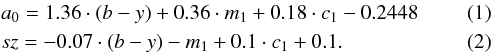 As
one can see from Fig. 2, a0 correlates
with Teff and sz correlates with
log g and
Teff. The photometric data were dereddened
with EB
− V = 003 (Carretta et al. 2000), using Eb −
y = 0.75·EB −
V.
As
one can see from Fig. 2, a0 correlates
with Teff and sz correlates with
log g and
Teff. The photometric data were dereddened
with EB
− V = 003 (Carretta et al. 2000), using Eb −
y = 0.75·EB −
V.
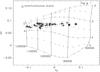 |
Fig. 2 Theoretical a0,sz grid as derived from Kurucz (1993) colours for [Fe/H] = −1.5. In addition, we show the positions of the cool blue HB stars (i.e. redward of the vertical line in Fig. 1) in this diagram as observed by Grundahl et al. (1999). |
Temperatures and surface gravities for stars redder than the u-jump that do not show evidence of radiative levitation as derived from the a0 and sz parameters and from line profile fits for an assumed metallicity of [M/H] = −1.5.
To restrict the fitting range we used only log g between 3 and 4 and Teff between 8000 K and 12 000 K. We fitted a second-order polynomial to the relation Teff (a0), which yielded an rms deviation of 30 K. For the surface gravities we fitted second-order polynomials to the relation log g (a0,sz), which yielded an rms deviation of 0.04 in log g. Temperatures and surface gravities derived from these relations are listed in Table 3 and plotted in Fig. 3 for stars cooler than the u-jump.
The errors provided in Table 3 are a quadratic
combination of errors from the photometric data, the uncertainty of the reddening in the
y-band
(estimated to be 002) and the
error of the fit to the theoretical relations. To estimate the influence of metallicity we
compared the results obtained for the two metallicities mentioned above. The differences
in temperature vary almost linearly from −0.1% at 8000 K to +0.8% at 12 000 K, with the results from the more metal-poor models
being hotter at the hot end. The differences are therefore well below the errors on the
individual temperatures.
The differences in surface gravities for these two metallicities show a quadratic dependency on the effective temperature, varying from +0.02 at about 8600 K (with the surface gravities from the metal-poor models being higher at 8600 K than those from the more metal-rich models) to 0 at 9000 K and 11 000 K via −0.02 at about 10 000 K. For temperatures below 8500 K the differences increase to −0.08, but these stars are too cool to be analysed spectroscopically with our methods (see Sect. 5.2). Within the temperature range of interest for further analysis the differences are below the average errors of the surface gravities given in Table 3. For reasons of consistency between photometric and spectroscopic analysis we decided against averaging the photometric grids.
From the errors listed in Table 3 and the uncertainties due to the metallicity, we estimate typical errors in Teff and log g to be about 5% and 0.13 dex, respectively.
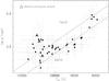 |
Fig. 3 Atmospheric parameters derived from the a0,sz indices for stars that do not show evidence for radiative levitation. For comparison we also show curves representing a canonical zero-age HB and terminal-age HB from Moehler et al. (2003). |
5.2. Line profile fitting with homogeneous model spectra
For stars redder than the u-jump, we computed model atmospheres with convection
for [M/H] = −1.5 using ATLAS9
(Kurucz 1993) and used Lemke’s
version of the LINFOR program (developed originally by Holweger, Steffen, and
Steenbock at Kiel University) to compute a grid of theoretical spectra that include the
Balmer lines H α to H22 and the He i and He ii lines. The
grid covers the range 7500 K ≤
Teff ≤ 12 000 K, 2.5 ≤ log g ≤ 5.0, and
 . For
stars bluer than the u-jump we used model atmospheres computed for
[M/H]=+0.5 (see Moehler et al. 2000 for details). From an extrapolation
of the LTE/NLTE threshold for subdwarf B stars (Napiwotzki
1997) we assumed that LTE is a valid approximation here as well. To establish the
best fit to the observed spectra, we used the fitsb2 routines developed by Napiwotzki et al. (2004), which employ a
χ2 test. The σ necessary to calculate
χ2 was estimated from the noise in the
continuum regions of the spectra. The fit program normalises synthetic model spectra
and observed spectra using the same points for the continuum
definition.
. For
stars bluer than the u-jump we used model atmospheres computed for
[M/H]=+0.5 (see Moehler et al. 2000 for details). From an extrapolation
of the LTE/NLTE threshold for subdwarf B stars (Napiwotzki
1997) we assumed that LTE is a valid approximation here as well. To establish the
best fit to the observed spectra, we used the fitsb2 routines developed by Napiwotzki et al. (2004), which employ a
χ2 test. The σ necessary to calculate
χ2 was estimated from the noise in the
continuum regions of the spectra. The fit program normalises synthetic model spectra
and observed spectra using the same points for the continuum
definition.
While the errors were obtained via boot strapping and should therefore be rather realistic, they do not include possible systematic errors due to flat-field inaccuracies or imperfect sky subtraction, for instance. The true errors in Teff are probably close to those from photometry, that is, 5%, and the true errors in log g are probably about 0.1.
Because the χ2 fit of the line profile can lead to ambiguous results for effective temperatures close to the Balmer maximum, the results from Sect. 5.1 were taken as initial parameters for the spectral line profile fitting procedure.
In Table 3 we list the results obtained from fitting the Balmer lines Hβ to H10 (excluding Hϵ to avoid the Ca ii H line) in the cool stars. For the cool stars we did not fit the helium lines because they are very weak and tend to produce spurious results. We verified, however, that the helium lines predicted by the model spectra with solar helium abundance did reproduce the observations. The reddest stars that showed many strong metal lines (55, 60, 61, 63, 72) were omitted from the line profile fits because our model spectra contain only H and He lines. In addition, we fitted the He i lines at λλ 4026 Å, 4388 Å, 4472 Å, and 4922 Å for stars hotter than 11 500 K.
Temperatures, surface gravities, and helium abundances from line profile fits for stars bluer than the u-jump that show evidence of radiative levitation.
Figure 4 shows a gap at 8500 K ≤ Teff ≤ 9000 K in the atmospheric parameters derived from line profile fitting, which was first noted and discussed by Moehler et al. (2003) for observations of HB stars in M 13. Stars populating this region in Fig. 3 close to the zero-age HB (ZAHB) are located at about 8000 K in Fig. 4, above the terminal-age HB (TAHB). Prompted by the referee, we treated a homogeneous model spectrum calculated for Teff = 8800 K,log g = 3.35 and [M/H] = −1.5 as described in Sect. 6.3 to simulate an observed spectrum. Varying the starting values of the fit from 8000 K to 9500 K for Teff and 3.2 to 3.6 for log g did not affect the fit results, which remained at Teff = 8841 K and log g = 3.35. Varying the FWHM of the Gaussian with which the model spectra are convolved before fitting from 0.6 Å to 0.75 Å resulted in Teff between 8818 K and 8862 K and log g between 3.34 and 3.36. We noted, however, that the resolution of the observed data seems to vary slightly with wavelength – at the blue end the predicted line profiles are very slightly wider and deeper than the observed ones, while for Hβ the observed line core is slightly more narrow and deep. To rule out possible small variations in resolution across the wavelength range as the cause for the gap, we convolved the observed spectra to a resolution of 2.5 Å, which is close to the resolution of the data of Moni Bidin et al. (2007, 2009, 2011) and Salgado et al. (2013), which do not show such a gap in their results, although they used the same analysis methods as we did. Unfortunately, the gap remains in the results of the line profile fitting. Using model atmospheres with or without convection did not affect the gap either.
The stars in Fig. 4 can be split into two groups with respect to their position relative to the evolutionary sequences: stars with effective temperatures between 9000 K and roughly 14 000 K lie between the ZAHB and the TAHB, while stars hotter or cooler than this temperature range lie above the TAHB.
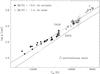 |
Fig. 4 Atmospheric parameters derived from the line profile fitting for stars hotter (full symbols) and cooler (open symbols) than the u-jump. For comparison we also show a canonical zero-age HB and terminal-age HB from Moehler et al. (2003). |
To determine how the parameters derived for the hot HB stars in NGC 288 differ from those obtained for other clusters and from the theoretical predictions we calculated the difference between the derived surface gravity and that on the ZAHB for the given temperature. Figure 5 compares our results with those obtained for M 80, NGC 5986 (Moni Bidin et al. 2009), NGC 6752 (Moni Bidin et al. 2007), M 22 (Salgado et al. 2013), and ω Cen (Moehler et al. 2011; Moni Bidin et al. 2011). Here the NGC 288 results resemble those from ω Cen for temperatures lower than 9000 K or higher than about 14 000 K, while they coincide with the other clusters for temperatures between 9000 K and 14 000 K.
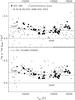 |
Fig. 5 Surface gravity relative to the zero-age HB at the given effective temperature. For comparison we also show a canonical zero-age and terminal-age HB from Moehler et al. (2003). In the upper plot we also show results from FORS2 observations of hot HB stars in M 80, NGC 5986 (Moni Bidin et al. 2009), NGC 6752 (Moni Bidin et al. 2007), and M 22 (Salgado et al. 2013). In the lower plot we also provide the results obtained from FLAMES and FORS2 observations of hot HB stars in ω Cen (Moehler et al. 2011, small squares; Moni Bidin et al. 2011, small triangles). |
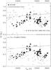 |
Fig. 6 Masses from line profile fits. For comparison we also show a canonical zero-age HB from Moehler et al. (2003). In the upper plot we also show results from FORS2 observations of hot HB stars in M 80, NGC 5986 (Moni Bidin et al. 2009), NGC 6752 (Moni Bidin et al. 2007), and M 22 (Salgado et al. 2013). In the lower plot we also provide the results obtained from FLAMES and FORS2 observations of hot HB stars in ω Cen (Moehler et al. 2011, small squares; Moni Bidin et al. 2011, small triangles). |
Using the spectroscopically determined atmospheric parameters, y-magnitudes, and the
distance modulus of the globular cluster ((m −
M)V = 1495, Carretta et al. 2000), we derived the masses shown in
Fig. 6 using the equation
![Mathematical equation: \begin{equation} {\frac{M}{M_\sun}} = {\frac{3.6\times10^{-7}}{\pi \cdot g_\sun \cdot R_\sun [{\rm pc}]}} \times 10^{-0.4 \cdot (y-(m-M)_V-y_{\rm th}),} \end{equation}](/articles/aa/full_html/2014/05/aa22953-13/aa22953-13-eq54.png) (3)where
yth is the theoretical y magnitude at the stellar
surface from Kurucz (1993) and R⊙ is the solar
radius in parsec. Obviously, the masses are systematically too low, except for stars just
hotter than the u-jump. Compared with results from other clusters,
the masses of the stars in NGC 288 show a similar behaviour as the surface gravities with
respect to HB stars in other globular clusters.
(3)where
yth is the theoretical y magnitude at the stellar
surface from Kurucz (1993) and R⊙ is the solar
radius in parsec. Obviously, the masses are systematically too low, except for stars just
hotter than the u-jump. Compared with results from other clusters,
the masses of the stars in NGC 288 show a similar behaviour as the surface gravities with
respect to HB stars in other globular clusters.
6. Abundances
We used the parameters derived in Sect. 5.2 for the following abundance analysis.
6.1. Helium
Helium abundances were already derived during the determination of effective temperatures
and surface gravities. In addition, we determined them (together with abundances for other
elements) via spectrum synthesis using the abundance-fitting routine of LINFOR (see
Sect. 6.2 for details). The resulting abundances
are listed in Tables 3 and 4. For the cool stars the abundances should be treated with caution
because the helium lines are rather weak. However, the average fitted helium abundance
 of −1.03 agrees well with our
assumption of solar helium abundance for cool stars. For hot stars the helium abundances
derived with LINFOR are in general slightly higher than those derived with fitsb2, but in
80% of the cases the difference is smaller than the error provided by fitsb2. On average,
the LINFOR abundances are higher by 0.06 dex, that is, much smaller than the error of the
fitsb2 results.
of −1.03 agrees well with our
assumption of solar helium abundance for cool stars. For hot stars the helium abundances
derived with LINFOR are in general slightly higher than those derived with fitsb2, but in
80% of the cases the difference is smaller than the error provided by fitsb2. On average,
the LINFOR abundances are higher by 0.06 dex, that is, much smaller than the error of the
fitsb2 results.
Because helium abundances have been derived for HB stars in many globular clusters with similar methods and model spectra as we used here, we compared our results with published data in Fig. 7. The helium abundances of Moni Bidin et al. (2007, 2009, 2012) and Moehler et al. (2000, 2003) were derived from low-resolution data with a resolution of 2.6−3.4 Å. The abundances of Behr (2003) were derived from data with a resolution of 0.1 Å, while the data used here have a resolution of about 0.7 Å. Between 11 000 K and 13 500 K the abundances show a clear correlation with the resolution of the data from which they were derived – the abundances decrease with increasing resolving power. This behaviour had been noticed already by Moni Bidin et al. (2012). This may be caused by the fact that at these relatively cool temperatures the helium lines are rather weak, which together with the helium deficiency makes them hard to fit. For higher temperatures the abundances from the different sources overlap, with the exception of the hottest star of Behr (2003). Due to the small number of results from high-resolution spectroscopy it is not clear whether the resolution effect persists to higher temperatures. For a comparison with predictions from diffusion theory see Sect. 6.4.
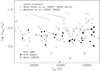 |
Fig. 7 Helium abundances for hot HB stars in M 80, NGC 5986, NGC 6752, and ω Cen (Moni Bidin et al.), M 3, M 13, and NGC 6752 (Moehler et al.) and NGC 288. The grey dots mark the abundances predicted for various HB ages from diffusion theory (with an ad hoc surface-mixing zone, Michaud et al. 2011, see Sect. 6.4 for details). The tracks have dots every 3 Myr. |
6.2. Heavy elements
Although the spectra have only medium resolution, we estimated abundances via spectrum synthesis using the abundance-fitting routine of LINFOR to verify whether our assumptions about the overall increase in heavy elements were roughly correct. We used the line lists from Kurucz (1993) and simultaneously determined abundances for He i, Mg ii, Si ii, P ii, Ti ii, Mn ii, Fe ii, and Ni ii. When the fitted abundances did not change anymore from one iteration to the next, we visually verified that the spectrum had indeed been well reproduced. The results are shown in Fig. 8. The LINFOR abundance-fitting routine only provides an overall error, but the scatter of abundances below 11 000 K gives an idea of the minimum uncertainties, because we do not expect the abundances shown in Fig. 8 to vary in these cool stars. For stars hotter than the u-jump additional uncertainties arise because we used homogeneous model atmospheres to analyse stars affected by diffusion.
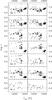 |
Fig. 8 Abundances derived via spectrum synthesis for all stars hotter than 9000 K. The triangles mark the same stars as in Fig. 1. The asterisks mark the results from Behr (2003). The bars at 17 500 K mark the average error bars of Behr (2003) for NGC 288. Our errors are probably not smaller. The dashed lines mark the solar abundances. The four-pointed stars mark the abundances derived for stratified model spectra (left column, see Sect. 6.3 for details), which indicate the equilibrium abundances achievable by diffusion. The grey dots (right column) mark the abundances predicted for various HB ages from diffusion theory (with an ad hoc surface-mixing zone, Michaud et al. 2011, see Sect. 6.4 for details). The tracks have dots every 1 Myr. |
The results for P ii, Ti ii, Mn ii, Fe ii, and Ni ii approximately agree with our assumption of [M/H] = +0.5 for stars hotter than the u-jump, while Mg ii and Si ii, on the other hand, are rather lower than our assumed abundances. However, since the atmospheric structure depends more on iron than on the light elements, we took these results to indicate that our assumptions were reasonable. For the cool stars, Mg ii and Ti ii seem to show an unexpected gradient with temperature, but it is unclear whether this is significant.
Our results show some differences compared with those obtained for NGC 288 by Behr (2003). Behr (2003) found no clear dependence of the Mg abundance relative to Teff for the three clusters studied with a sufficient number of stars with Teff above the u-jump, while a trend appears to be present in our results for NGC 288. For Si and Mn Behr found significantly lower abundances than we do, which might be an effect of instrumental resolution (see Sect. 6.1). The observed abundances shown in Fig. 8 are provided at the CDS.
6.3. Abundances predicted by stratified model spectra
To compare the results from our observed spectra with the predictions from stratification theory we also determined abundances from model spectra of LeBlanc et al. (2009), which include abundance stratification due to diffusion. These models self-consistently calculate the structure of the atmosphere with the vertical abundance stratification. The abundances of the individual elements are calculated in each layer of the atmosphere while assuming equilibrium (nil diffusion-velocity). This leads to vertical abundance stratification and modifies the atmospheric structure. First we compared the observed metal lines with those predicted by stratification models and found that the observed lines were much weaker than predicted by these models (see Fig. 9).
As discussed in LeBlanc et al. (2009), the abundances of some elements (Fe, for example) predicted by the models can be overestimated because in a real star the diffusion process is a time-dependent phenomenon. Even though the radiative forces on a given element can theoretically support a very large overabundance, this situation may be hampered by various factors. The equilibrium solution used in these models may therefore not be reached. For instance, in a real star, such a large quantity of atoms might not be able to surface due to the diffusion that takes place below the stellar atmosphere. In addition, the abundances of other elements (such as helium) that have relatively weak radiative accelerations can be underestimated by these models.
Next we convolved the stratified model spectra to the same resolution as our observed data and multiplied them with a spectrum of average 1 and rms of 0.0125, resulting in a signal-to-noise ratio of 80. Then we determined their effective temperatures and surface gravities in the same way as described in Sect. 5.2, except that we used a model grid with [M/H] = +1, since the lines in the stratified model spectra were much stronger than in the observed spectra (see Fig. 9). The resulting parameters are given in Table 5 and clearly show that the analysis of stratified model spectra with homogeneous model spectra yields lower temperatures and surface gravities, with the difference in temperature increasing with increasing temperature.
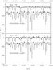 |
Fig. 9 Normalised spectra for stars 199 (upper panel, 12 400 K) and 221 (lower panel, 13 400 K) compared with stratified model spectra F (upper panel) and H (lower panel), which have fitted parameters close to those of the observed spectra. For clarity, the stratified model spectra have been offset by 0.1 from the observed spectra (see Tables 4 and 5). |
Using the parameters in the right column of Table 5, we then determined abundances for the model spectra with fitted log g above 3.45 as expected for stars on or near the ZAHB at the fitted temperatures, that is, all models except A and D. We alternated between simultaneously fitting the ions Mg ii, Si ii, P ii, S ii, A ii, Ti ii, V ii, Cr ii, and simultaneously fitting the ions Mn ii, Fe i, Fe ii, Co ii, Ni ii, Sr ii, and Zr ii, until the fit did not improve any more. Then we again visually checked that most of the spectrum had been reproduced. Typically, we found that some lines were not fit well, but that was to be expected since the abundance distribution in the model atmospheres creating these spectra is far from homogeneous, which results in a very different atmospheric structure. The results of these fits are marked by four-pointed stars in the left column of Fig. 8. As already suggested by the comparison shown in Fig. 9, the abundances derived from the stratified spectra are generally higher than those derived from the observed spectra, with He i (virtually absent from stratified model atmospheres) and Mg ii being the exceptions.
6.4. Abundances predicted by diffusion models
It is also possible to compare our abundance results with stellar evolution models computed including the effects of atomic diffusion (Michaud et al. 2008, 2011). These models followed the evolution from the zero-age main sequence, treating in detail atomic diffusion inside the star. On the HB, they predicted large overabundances of metals, often larger than observed above 11 000 K (similar to the problems found above for the stratified model atmospheres). A surface mixed mass of around 10-7M⊙ was needed to reduce the expected anomalies to values observed in HB stars of a number of clusters as well as in sdB stars. However, the introduction of a surface mixing layer leads to a vertically homogeneous atmosphere. This contradicts the observed vertical stratification of certain elements, including iron, in some blue HB stars (Khalack et al. 2007, 2008, 2010). The tracks shown in Fig. 8 are taken from Michaud et al. (2011). These tracks start with the original cluster abundances at the ZAHB and cover the first third of horizontal branch evolution, which lasts some 100 Myr2.
Figure 8 shows that the abundances change more rapidly during the first 10 Myr than during the following 20 Myr for all species that become overabundant. This is largely caused by a reduction of the radiative accelerations as the concentrations increase. The abundance increase is also expected to be slow during the following 70 Myr for these species. The Si, Ti, Fe, and Ni observations are within the expected abundance range when one takes error bars evaluated from the scatter of Fe and Si below 11 000 K into account. For Si, the trend suggested by the models appears to be present in the data. For Mn our abundances are higher than the results from Behr (2003), which agree well with the predictions. Phosphorus is some five times more overabundant than predicted by the models, whereas magnesium shows small effects, while the models predict about five times larger abundances.
Helium is observed to be more underabundant than expected after 30 Myr (cf. Fig. 7). However, its abundance has a very different time dependence from that of metals. The underabundance of helium is caused by gravitational settling, and this process is as rapid from 10 to 30 Myr as during the first 10 Myr. Because helium settles, the settling goes as e−t/θ, where θ is the settling time scale. This means that the settling continues exponentially, and if helium is underabundant by a factor of 3 after 30 Myr it should be underabundant by a factor of around 27 after 100 Myr, corresponding to a value of 9.56 in Fig. 8 at the end of the HB evolution. Because it is highly unlikely, however, that most of the stars in Fig. 8 are at the end of their HB evolution, some discrepancy remains.
As may be seen from Fig. 4 of Michaud et al. (2011), abundance anomalies caused by atomic diffusion are not limited to a thin surface phenomenon. However, there are species (e.g. Mg) whose observed anomalies do not agree with the expected ones, suggesting that the model may be missing something. Assuming that the outer 10-7M⊙ is completely mixed could be an oversimplification, especially since the mixing mechanism is currently unknown. For instance, it might be thermohaline convection (see Sect 5.3 of Michaud et al. 2011). This is a relatively weak convection that might not eliminate all effects of additional diffusion in the atmosphere. For instance, helium is largely neutral in the atmosphere of HB stars of 11 000 K to 15 000 K so that it has an atomic diffusion coefficient larger than that of ionized metals (by a factor of around 100); helium might then be the most affected atomic species as turbulence weakens. This remains speculative.
7. Line profile fitting with stratified model spectra
We also examined how the use of stratified instead of homogeneous model atmospheres to fit
our observations influenced the parameters determined from these fits. To allow a direct
comparison with results obtained using homogeneous model spectra without metal lines to fit
our observations, we calculated a set of synthetic spectra with only H present (the
abundance of all of the other elements were set at −5.00, while H was at 12.00) while using the
relations between temperature, density, and radius from the stratified model atmospheres.
Helium lines were not included because the stratification abundances of helium are extremely
low. For comparison, we also fitted the observed spectra again (only H lines) with
homogeneous model spectra computed with [M/H] = +0.5 and
= −3. The results are shown in
Fig. 10. The prediction of higher spectroscopic
gravities by the models including abundance stratification shown here was also found in
Hui-Bon-Hoa et al. (2000) and LeBlanc et al. (2010). The amplitude of the effect might be overestimated
by the stratified models because in most cases, they predict stronger abundance anomalies
for blue HB stars than observed (see Sect. 6).
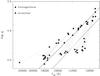 |
Fig. 10 Atmospheric parameters derived from the line profile fitting for stars hotter than
the u-jump, using homogeneous model atmospheres ([M/H]
= +0.5,
|

In Fig. 10 all stars move to higher temperatures and surface gravities when fitted with model spectra from stratified model atmospheres (as expected from the results of the reverse fitting given in Table 5), but only stars between 14 000 K and 16 000 K move closer to the ZAHB. Cooler stars show too high surface gravities, while hotter ones move parallel to the TAHB. The principal defect of the stratified models is that they generally predict larger abundances than observed. In more realistic models, one would expect that the shifts shown in Fig. 10 be somewhat smaller. The lower temperature stars could then possibly fall between the TAHB and ZAHB in the log g − Teff plane, which would give satisfactory results.
As a consistency check we derived masses for the new parameters, adjusting the theoretical
y-magnitudes
of Kurucz (1993) for [M/H] = +0.5 by −03 to account for
the stratification effects. This offset was determined by comparing the fluxes of stratified
and homogeneous model spectra. The results are shown in Fig. 11. Here the values obtained from stratified model spectra for stars above
14 000 K are now closer to the canonical values than those obtained from homogeneous model
spectra. This provides some support to the notion that the too low surface gravities and
masses found from analyses with homogeneous model spectra are caused by the mismatch in
atmospheric structure between homogeneous and stratified model atmospheres. One should keep
in mind, however, that the stratified model atmospheres in general predict much stronger
lines than observed, therefore it is currently unclear whether a fully self-consistent
solution can be achieved. Similarly to the discussion related to the large shifts found in
Fig. 10, the masses predicted in Fig. 11 by more realistic stratified models for stars just
above the temperature threshold of the u-jump, in which the abundances are less extreme,
would be closer to the ZAHB.
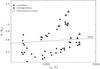 |
Fig. 11 Masses determined from line profile fits for stars bluer than the Grundahl jump, using homogeneous (filled circles) and stratified (filled triangles) model spectra. |
8. Overluminous stars
One possible explanation for the overluminous stars mentioned in Sect. 1 is that they have evolved from hotter locations blueward of the u-jump and are now near the end of their HB phase, evolving towards the asymptotic giant branch. Because the evolution away from the zero-age HB increases the overall luminosity of an HB star, one would expect such evolved stars to be overluminous in other bandpasses in addition to u compared with stars near the zero-age HB. Figure 12 shows the relation between the effective temperature derived from line profile fits and the y-magnitude of the HB stars. Here especially the hot overluminous stars are clearly brighter than the “normal” stars at similar temperatures. To a lesser extent, this is also true for the cool overluminous stars. In Figs. 4 and 5, however, only three of the overluminous stars, namely 100 (hot), 103, and 127 (both cool) are clearly separated from the majority of the stars by a significantly lower surface gravity. It is unclear why the other overluminous stars have higher luminosities, because they are inconspicuous with respect to the majority of the stars in all other parameters (effective temperature, surface gravity, and abundances). However, even three stars evolving off the ZAHB in the temperature range 9700 K to 11 500 K pose a problem for evolutionary time-scales, as one would expect to find about 100 HB stars close to the ZAHB between about 11 000 K and 14 000 K (corresponding to a range of roughly 0.5−1.05 in u − y in Fig. 1) for each of the evolved stars, which is clearly not the case.
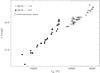 |
Fig. 12 The y-magnitudes of the HB stars compared with the effective temperatures derived from line profile fits. |
If the overluminous stars are post-HB stars evolved from a hotter location along the blue tail (as suggested by their higher luminosity), one would expect them to preserve their abundance anomalies during their evolution towards cooler temperatures until dredge-up from the deepening hydrogen convection zone, which causes the surface abundances to return to approximately the normal cluster abundances. However, such stars are expected to have had a low He abundance on the HB and a low rotation rate, which may cause them to maintain their abundance anomalies to temperatures somewhat lower than the u-jump. First, due to the depletion of their surface helium, the overluminous stars just redward of the u-jump may have slightly shallower convection zones than other stars of the same effective temperature. However, hydrogen ionization is the main driver of the convection when the effective temperature is lower than 10 000 K and it will lead to progressive helium dredge-up so that the difference in convection zone depth could be small below 10 000 K. Second, because of the rotation-rate drop in HB stars blueward of the u-jump, the overluminous stars would be expected to have low rotation rates if they are evolved from the blue HB. This, in turn, would reduce the meridional flows that inhibit diffusion in stars cooler than the u-jump. However, as may be seen from Fig. 4 of Quievy et al. (2009), the limiting rotation rate decreases very rapidly as the effective temperature drops below 10 000 K; a star with a ve = 8 km s-1 would show strong effects of diffusion above 12 000 K but would be mixed below 10 000 K. The results given in Fig. 8 indeed show that the effects of radiative diffusion disappear between the overluminous stars hotter than the u-jump at 11 500 K and the overluminous stars cooler than the u-jump at 10 000 K. Accordingly, the low He abundance due to diffusion and low rotation apparently does not prevent the effects of diffusion from disappearing rather quickly as a star evolves through the u-jump region to cooler temperatures. This result supports the general assumption that the abundances of HB stars redward of the u-jump are not affected by diffusion, irrespective of their evolutionary status. The observations are ahead of the stellar evolution models in this case. To set the theory on a stronger base, the evolution calculations with diffusion need to be continued to the end of the HB; but meridional circulation needs to be included as well to verify at which effective temperature the mixing occurs and how this temperature depends on rotation.
9. Summary and conclusions
-
The atmospheric parameters and masses of the hot HB stars in NGC 288 show a behaviour also seen in other clusters for temperatures between 9000 K and 14 000 K. Outside this temperature range, however, they follow the results found for such stars in ω Cen.
-
The abundances derived from our observations are for most elements within the abundance range expected from evolutionary models that include the effects of atomic diffusion and assume a surface mixed mass of 10-7M⊙, as determined previously for sdB stars and other clusters. The exceptions are helium, which is more deficient than expected, and phosphorus, which is substantially more abundant than predicted. The abundances predicted by stratified model atmospheres, which were not adjusted to observations, are generally significantly more extreme than observed, except for magnesium.
-
When the observed spectra were analysed with stratified model spectra, the HB stars were moved to higher temperatures, surface gravities, and masses. Since the equilibrium abundances led to excessive adjustments, more realistic abundance gradients may well lead to models that locate the HB stars between the TAHB and ZAHB (see Sect. 7). Model atmospheres including such improvements are needed to answer this question.
-
Five of the eight overluminous stars around the u-jump that we observed do not deviate substantially from the other HB stars in the same temperature range in any of the parameters we determined. We are therefore at a loss to explain their brighter luminosities. The remaining three overluminous stars do show lower surface gravities, as would be expected if they evolved away from the HB. However, they pose a substantial problem for evolutionary time-scales, because one would expect to find approximately100 HB stars close to the ZAHB between about 11 000 K and 14 000 K (corresponding to a range of roughly 0.5−1.05 in u − y in Fig. 1) for each of the evolved stars, which is clearly not the case.
-
All overluminous stars show the same abundance behaviour as the majority of the stars in the respective temperature range. This result supports the general assumption that the abundances of HB stars redward of the u-jump are not affected by diffusion, irrespective of their evolutionary status.
Evolution models including diffusion and stratified model atmospheres both predict higher-than-observed abundances for many elements affected by radiative levitation. Evolution models can be adjusted to reproduce the observed abundances by introducing an ad hoc defined mixed zone, which is potentially inconsistent with the observed vertical stratification of at least some elements in the atmosphere, however. For stratified model atmospheres it is currently unclear whether a more limited abundance stratification, which would provide a better description of the observed abundances, would still be able to explain the photometric anomalies around the u-jump. Our results show definite promise towards solving the long-standing problem of surface gravity and mass discrepancies for hot HB stars, but much work is still needed to arrive at a self-consistent solution.
Online material
Target coordinates and photometric data.
Observing times, conditions, and setups.
The models around 12 000 and 13 500 K were stopped around 10 Myr because of convergence problems, but the trend can be estimated from the surrounding models.
Acknowledgments
We thank André Drews for his careful reduction of the data. We are grateful to Christian Moni Bidin for sending his results to allow direct comparisons and for providing a very thorough and helpful referee report.
References
- Behr, B. B. 2003, ApJS, 149, 67 [NASA ADS] [CrossRef] [Google Scholar]
- Behr, B. B., Cohen, J. G., McCarthy, J. K., & Djorgovski, S. G. 1999, ApJ, 517, L135 [NASA ADS] [CrossRef] [Google Scholar]
- Behr, B. B., Cohen, J. G., & McCarthy, J. K. 2000a, ApJ, 531, L37 [NASA ADS] [CrossRef] [PubMed] [Google Scholar]
- Behr, B. B., Djorgovski, S. G., Cohen, J. G., et al. 2000b, ApJ, 528, 849 [NASA ADS] [CrossRef] [Google Scholar]
- Carretta, E., Gratton, R. G., Clementini, G., & FusiPecci, F. 2000, ApJ, 533, 215 [NASA ADS] [CrossRef] [Google Scholar]
- Carretta, E., Bragaglia, A., Gratton, R., D’Orazi, V., & Lucatello, S. 2009a, A&A, 508, 695 [NASA ADS] [CrossRef] [EDP Sciences] [Google Scholar]
- Carretta, E., Bragaglia, A., Gratton, R., & Lucatello, S. 2009b, A&A, 505, 139 [NASA ADS] [CrossRef] [EDP Sciences] [Google Scholar]
- Carretta, E., Bragaglia, A., Gratton, R., D’Orazi, V., & Lucatello, S. 2011, A&A, 535, A121 [NASA ADS] [CrossRef] [EDP Sciences] [Google Scholar]
- Crocker, D. A., Rood, R. T., & O’Connell, R. W. 1988, ApJ, 332, 236 [NASA ADS] [CrossRef] [Google Scholar]
- Drews, A. 2005, Diploma Thesis, Christian-Albrechts Universität Kiel [Google Scholar]
- Fabbian, D., Recio-Blanco, A., Gratton, R. G., & Piotto, G. 2005, A&A, 434, 235 [NASA ADS] [CrossRef] [EDP Sciences] [Google Scholar]
- Ferraro, F. R., Paltrinieri, B., Pecci, F. F., et al. 1998, ApJ, 500, 311 [NASA ADS] [CrossRef] [Google Scholar]
- Gratton, R. G., Carretta, E., Bragaglia, A., Lucatello, S., & D’Orazi, V. 2010, A&A, 517, A81 [NASA ADS] [CrossRef] [EDP Sciences] [Google Scholar]
- Grundahl, F., Catelan, M., Landsman, W. B., Stetson, P. B., & Andersen, M. I. 1999, ApJ, 524, 242 [NASA ADS] [CrossRef] [Google Scholar]
- Harris, W. E. 1996, AJ, 112, 1487 (version Dec. 2010) [NASA ADS] [CrossRef] [Google Scholar]
- Horne, K. 1986, PASP, 98, 609 [NASA ADS] [CrossRef] [EDP Sciences] [Google Scholar]
- Hui-Bon-Hoa, A., LeBlanc, F., & Hauschildt, P. H. 2000, ApJ, 535, L43 [NASA ADS] [CrossRef] [PubMed] [Google Scholar]
- Khalack, V. R., LeBlanc, F., Bohlender, D., Wade, G. A., & Behr, B. B. 2007, A&A, 466, 667 [NASA ADS] [CrossRef] [EDP Sciences] [Google Scholar]
- Khalack, V. R., LeBlanc, F., Behr, B. B., Wade, G. A., & Bohlender, D. 2008, A&A, 477, 641 [NASA ADS] [CrossRef] [EDP Sciences] [Google Scholar]
- Khalack, V., LeBlanc, F., & Behr, B. B. 2010, MNRAS, 407, 1767 [NASA ADS] [CrossRef] [Google Scholar]
- Kurucz, R. L. 1993, ATLAS9 Stellar Atmospheres Program and 2 km s-1 grid, CR-ROM No. 13 [Google Scholar]
- Lane, R. R., Kiss, L. L., Lewis, G. F., et al. 2010, MNRAS, 406, 2732 [NASA ADS] [CrossRef] [Google Scholar]
- LeBlanc, F., Monin, D., Hui-Bon-Hoa, A., & Hauschildt, P. H. 2009, A&A, 495, 937 [NASA ADS] [CrossRef] [EDP Sciences] [Google Scholar]
- LeBlanc, F., Hui-Bon-Hoa, A., & Khalack, V. R. 2010, MNRAS, 409, 1606 [NASA ADS] [CrossRef] [Google Scholar]
- Michaud, G., Vauclair, G., & Vauclair, S. 1983, ApJ, 267, 256 [NASA ADS] [CrossRef] [Google Scholar]
- Michaud, G., Richer, J., & Richard, O. 2008, ApJ, 675, 1223 [NASA ADS] [CrossRef] [Google Scholar]
- Michaud, G., Richer, J., & Richard, O. 2011, A&A, 529, A60 [NASA ADS] [CrossRef] [EDP Sciences] [Google Scholar]
- Moehler, S. 2001, PASP, 113, 1162 [NASA ADS] [CrossRef] [Google Scholar]
- Moehler, S., Heber, U., & de Boer, K. S. 1995, A&A, 294, 65 [NASA ADS] [Google Scholar]
- Moehler, S., Heber, U., & Rupprecht, G. 1997, A&A, 319, 109 [NASA ADS] [Google Scholar]
- Moehler, S., Sweigart, A. V., Landsman, W. B., & Heber, U. 2000, A&A, 360, 120 [NASA ADS] [Google Scholar]
- Moehler, S., Landsman, W. B., Sweigart, A. V., & Grundahl, F. 2003, A&A, 405, 135 [NASA ADS] [CrossRef] [EDP Sciences] [Google Scholar]
- Moehler, S., Dreizler, S., Lanz, T., et al. 2011, A&A, 526, A136 [NASA ADS] [CrossRef] [EDP Sciences] [Google Scholar]
- Monelli, M., Milone, A. P., Stetson, P. B., et al. 2013, MNRAS, 431, 2126 [NASA ADS] [CrossRef] [Google Scholar]
- Moni Bidin, C., Moehler, S., Piotto, G., Momany, Y., & Recio-Blanco, A. 2007, A&A, 474, 505 [NASA ADS] [CrossRef] [EDP Sciences] [Google Scholar]
- Moni Bidin, C., Moehler, S., Piotto, G., Momany, Y., & Recio-Blanco, A. 2009, A&A, 498, 737 [NASA ADS] [CrossRef] [EDP Sciences] [Google Scholar]
- Moni Bidin, C., Villanova, S., Piotto, G., Moehler, S., & D’Antona, F. 2011, ApJ, 738, L10 [NASA ADS] [CrossRef] [Google Scholar]
- Moni Bidin, C., Villanova, S., Piotto, G., et al. 2012, A&A, 547, A109 [NASA ADS] [CrossRef] [EDP Sciences] [Google Scholar]
- Moon, T. T., & Dworetsky, M. M. 1985, MNRAS, 217, 305 [NASA ADS] [CrossRef] [Google Scholar]
- Napiwotzki, R. 1997, A&A, 322, 256 [NASA ADS] [Google Scholar]
- Napiwotzki, R., Yungelson, L., Nelemans, G., et al. 2004, in Spectroscopically and Spatially Resolving the Components of the Close Binary Stars, eds. R. W. Hilditch, H. Hensberge, & K. Pavlovski, ASP Conf. Ser., 318, 402 [Google Scholar]
- Pace, G., Recio-Blanco, A., Piotto, G., & Momany, Y. 2006, A&A, 452, 493 [NASA ADS] [CrossRef] [EDP Sciences] [Google Scholar]
- Pasquini, L., Avila, G., Allaert, E., et al. 2000, in Optical and IR Telescope Instrumentation and Detectors, eds. M. Iye, & A. F. Moorwood, SPIE Conf. Ser., 4008, 129 [Google Scholar]
- Peterson, R. C., Rood, R. T., & Crocker, D. A. 1995, ApJ, 453, 214 [NASA ADS] [CrossRef] [Google Scholar]
- Piotto, G., Milone, A. P., Marino, A. F., et al. 2013, ApJ, 775, 15 [NASA ADS] [CrossRef] [Google Scholar]
- Quievy, D., Charbonneau, P., Michaud, G., & Richer, J. 2009, A&A, 500, 1163 [NASA ADS] [CrossRef] [EDP Sciences] [Google Scholar]
- Roh, D.-G., Lee, Y.-W., Joo, S.-J., et al. 2011, ApJ, 733, L45 [NASA ADS] [CrossRef] [Google Scholar]
- Salgado, C., Moni Bidin, C., Villanova, S., Geisler, D., & Catelan, M. 2013, A&A, 559, A101 [NASA ADS] [CrossRef] [EDP Sciences] [Google Scholar]
- Székely, P., Kiss, L. L., Szatmáry, K., et al. 2007, Astron. Nachr., 328, 879 [NASA ADS] [CrossRef] [Google Scholar]
- ten Bruggencate, P. 1927, Sternhaufen (Berlin: Springer) [Google Scholar]
- Tonry, J., & Davis, M. 1979, AJ, 84, 1511 [NASA ADS] [CrossRef] [Google Scholar]
- Yong, D., Grundahl, F., Johnson, J. A., & Asplund, M. 2008, ApJ, 684, 1159 [NASA ADS] [CrossRef] [Google Scholar]
All Tables
Temperatures and surface gravities for stars redder than the u-jump that do not show evidence of radiative levitation as derived from the a0 and sz parameters and from line profile fits for an assumed metallicity of [M/H] = −1.5.
Temperatures, surface gravities, and helium abundances from line profile fits for stars bluer than the u-jump that show evidence of radiative levitation.
All Figures
|
Fig. 1 Blue HB stars in NGC 288 as observed by Grundahl et al. (1999). The subsample, for which GIRAFFE spectra were observed, is marked by filled circles. The dot-dashed line in the left part marks the u − y colour of the u-jump. Stars on the red side of the line do not show evidence for radiative levitation, while stars on the blue side do. The triangles mark overluminous stars around the u-jump (from red to blue: 122, 103, 127, 101, 146, 142, 100, 183). |
| In the text | |
|
Fig. 2 Theoretical a0,sz grid as derived from Kurucz (1993) colours for [Fe/H] = −1.5. In addition, we show the positions of the cool blue HB stars (i.e. redward of the vertical line in Fig. 1) in this diagram as observed by Grundahl et al. (1999). |
| In the text | |
|
Fig. 3 Atmospheric parameters derived from the a0,sz indices for stars that do not show evidence for radiative levitation. For comparison we also show curves representing a canonical zero-age HB and terminal-age HB from Moehler et al. (2003). |
| In the text | |
|
Fig. 4 Atmospheric parameters derived from the line profile fitting for stars hotter (full symbols) and cooler (open symbols) than the u-jump. For comparison we also show a canonical zero-age HB and terminal-age HB from Moehler et al. (2003). |
| In the text | |
|
Fig. 5 Surface gravity relative to the zero-age HB at the given effective temperature. For comparison we also show a canonical zero-age and terminal-age HB from Moehler et al. (2003). In the upper plot we also show results from FORS2 observations of hot HB stars in M 80, NGC 5986 (Moni Bidin et al. 2009), NGC 6752 (Moni Bidin et al. 2007), and M 22 (Salgado et al. 2013). In the lower plot we also provide the results obtained from FLAMES and FORS2 observations of hot HB stars in ω Cen (Moehler et al. 2011, small squares; Moni Bidin et al. 2011, small triangles). |
| In the text | |
|
Fig. 6 Masses from line profile fits. For comparison we also show a canonical zero-age HB from Moehler et al. (2003). In the upper plot we also show results from FORS2 observations of hot HB stars in M 80, NGC 5986 (Moni Bidin et al. 2009), NGC 6752 (Moni Bidin et al. 2007), and M 22 (Salgado et al. 2013). In the lower plot we also provide the results obtained from FLAMES and FORS2 observations of hot HB stars in ω Cen (Moehler et al. 2011, small squares; Moni Bidin et al. 2011, small triangles). |
| In the text | |
|
Fig. 7 Helium abundances for hot HB stars in M 80, NGC 5986, NGC 6752, and ω Cen (Moni Bidin et al.), M 3, M 13, and NGC 6752 (Moehler et al.) and NGC 288. The grey dots mark the abundances predicted for various HB ages from diffusion theory (with an ad hoc surface-mixing zone, Michaud et al. 2011, see Sect. 6.4 for details). The tracks have dots every 3 Myr. |
| In the text | |
|
Fig. 8 Abundances derived via spectrum synthesis for all stars hotter than 9000 K. The triangles mark the same stars as in Fig. 1. The asterisks mark the results from Behr (2003). The bars at 17 500 K mark the average error bars of Behr (2003) for NGC 288. Our errors are probably not smaller. The dashed lines mark the solar abundances. The four-pointed stars mark the abundances derived for stratified model spectra (left column, see Sect. 6.3 for details), which indicate the equilibrium abundances achievable by diffusion. The grey dots (right column) mark the abundances predicted for various HB ages from diffusion theory (with an ad hoc surface-mixing zone, Michaud et al. 2011, see Sect. 6.4 for details). The tracks have dots every 1 Myr. |
| In the text | |
|
Fig. 9 Normalised spectra for stars 199 (upper panel, 12 400 K) and 221 (lower panel, 13 400 K) compared with stratified model spectra F (upper panel) and H (lower panel), which have fitted parameters close to those of the observed spectra. For clarity, the stratified model spectra have been offset by 0.1 from the observed spectra (see Tables 4 and 5). |
| In the text | |
|
Fig. 10 Atmospheric parameters derived from the line profile fitting for stars hotter than
the u-jump, using homogeneous model atmospheres ([M/H]
= +0.5,
|
| In the text | |
|
Fig. 11 Masses determined from line profile fits for stars bluer than the Grundahl jump, using homogeneous (filled circles) and stratified (filled triangles) model spectra. |
| In the text | |
|
Fig. 12 The y-magnitudes of the HB stars compared with the effective temperatures derived from line profile fits. |
| In the text | |
Current usage metrics show cumulative count of Article Views (full-text article views including HTML views, PDF and ePub downloads, according to the available data) and Abstracts Views on Vision4Press platform.
Data correspond to usage on the plateform after 2015. The current usage metrics is available 48-96 hours after online publication and is updated daily on week days.
Initial download of the metrics may take a while.