| Issue |
A&A
Volume 564, April 2014
|
|
|---|---|---|
| Article Number | A117 | |
| Number of page(s) | 17 | |
| Section | Catalogs and data | |
| DOI | https://doi.org/10.1051/0004-6361/201323238 | |
| Published online | 16 April 2014 | |
A whole sky study of quasars known population starting from the LQAC-2 compiled catalogue
Observatoire de Paris, SYRTE, CNRS/UMR 8630,
75014
Paris,
France
e-mail:
This email address is being protected from spambots. You need JavaScript enabled to view it.
Received:
12
December
2013
Accepted:
22
February
2014
Abstract
Context. Thanks to huge surveys, such as the Sloan Digital Sky Survey (SDSS), the last decade has shown a dramatic increase in the number of known quasars. In the second release of the general compiled catalogue Large Quasar Astrometric Catalogue (LQAC), 187 504 objects are recorded.
Aims. From this catalogue, we carry out statistical studies dealing with several topics: the astrometric accuracy of the quasars, their spatial location, the distribution of the distance to the closest neighbour, the identification of binary quasars, the completness of catalogues at a given magnitude and the estimation of the number of quasars expected to be detected by the astrometric space mission Gaia.
Methods. We analyse the astrometric improvements brought by the LQAC-2 in terms of equatorial coordinates off-sets. We plot the bi-dimensional spatial distribution of the LQAC-2 quasars according to their equatorial, galactic, and ecliptic coordinates, thus exploring the anisotropy of the distribution. We compare the observed distribution of closest neighbours with the theoretical values based on a Poisson distribution. Moreover, we perform a comparison between two catalogues, the SDSS and the 2dF inside a huge common field. By extrapolating to the whole sky we deduce the number of quasars that will be detected by Gaia.
Results. We show how the equatorial, ecliptic, and galactic distribution of recorded quasars is strongly affected by the galactic extinction as well as by the deficiency of detections in the southern hemisphere. In homogenous zones covered by the SDSS survey we identify a significant excess of closest neighbours at short angular distances, with respect to the theoretical estimation, which is caused by the presence of binary quasars. Moreover, we detail the incompletness of systematic survey catalogues at any magnitude threshold, when comparing two huge surveys such as the SDSS and 2dF. Following this study we deduce the number of quasars detected by Gaia under a given magnitude threshold. For V = 20, this number should be at least 1 million objects.
Key words: quasars: general / catalogs / astrometry
© ESO, 2014
1. Introduction
In the recent years, the number of recorded quasars has significantly increased. It reached 151 217 objects in the last and thirteenth. release of the Véron-Cetty & Véron (2010) compilation (when adding BL LAC objects and Seyfert 1 galaxies to true QSO’s), and 187 504 objects in the second release of the Large Quasar Astrometric Catalogue (LQAC-2) constructed by Souchay et al. (2012). A priori, the distribution of the objects already detected is far from homogeneous in the whole celestial sphere because of the variety of original surveys involved in these compilated catalogues with inhomogeneous sky coverage and magnitude thresholds. Nevertheless, a catalogue like the LQAC-2 gives the opportunity to carry out some statistical studies of the recorded quasar population in the whole sky as well as in some well delimited and homogeneous areas. It also helps to estimate the level of incompletness of the available data as well as the inhomogeneities in the sky distribution of the objects recorded so far. This is the main purpose of this paper.
We carry out our study starting from the LQAC-2 compiled catalogue. Recall that one of its main objectives was to recompute the equatorial coordinates of the quasars of the compilation from algorithms leading to an optimized accuracy of the positions of the objects. These algorithms were exactly those used in the construction of the Large Quasar Reference Frame (LQRF) by Andrei et al. (2009). In addition, the LQAC-2 contains extended multi-bands photometry, radiofluxes, redshifts, a new calculation of the absolute magnitudes in two bands (b and i), and finally a morphological characterization of the quasars from three estimators (skewness, roundness, and normalness).
2. Astrometric improvement
One of the main aims of the LQAC, and more specifically of its second release the LQAC-2, was to recalculate the equatorial coordinates of the quasars compiled in the various catalogues included in the compilation in a more accurate manner. Of course, we could exclude from this re-calculation the catalogues of radio quasars observed with the Very-Long-Baseline Interferometry (VLBI) technique, which give positions of the objects at the level of milliarcseconds. These include the 3414 quasars of the International Celestial Reference Frame (ICRF2, Ma et al. 2009; Bobholtz et al. 2010), 5198 from the Very Long Baseline Array (VLBA), 1858 from the Very Large Array (VLA, Claussen 2006) and 2118 from Jodrell Bank-VLA Astrometric Survey (JVAS). Notice that the positional off-set between the radio VLBI centre and the photocentre of these quasars is subject to particular recent investigations (Orosz & Frey 2013; Zacharias & Zacharias 2014). These objects with optimal astrometric quality at radio wavelengths represent only a small part of the LQAC-2. The four catalogues concerned gather no more than 5717 quasars with respect to the 187 504 quasars of the whole LQAC-2, that is to say, a mere 3.05%. Thus, although the objects concerned are fundamental in terms of astrometric standards and references, their relative proportion is very small.
2.1. Recomputation of equatorial coordinates from the LQRF
Except in the case of the specific VLBI sample mentioned above, the positions of the objects found in the original catalogues belonging to the compilation are subject to a lack of accuracy, sometimes at the level of a few tenths of arcsecond or even a few arcseconds (Souchay et al. 2009), which explains the necessity of a recomputation of their equatorial coordinates. This was done through the intermediary of the algorithms taken to construct the LQRF (Andrei et al. 2009). They consist in homogenizing astromery and reaching the milliarcsecond alignment with the ICRF. In these algorithms, the quasars are found, when available, in the very large optical surveys as the USNO B1.0 (Monet et al. 2003), the GSC2.3 (Lasker et al. 2008), and the Sloan Digital Sky Survey (SDSS). The positions were then placed onto the UCAC-2 based reference frame (Zacharias et al. 2004). A final step consisted in using spherical harmonics to fit the coordinates with the ICRF2. All this recomputation procedure was possible only for the quasars which could offer a counterpart in one or more of the various surveys used in the algorithm above. This concerns 159 700 objects, i.e., 85.17% of the whole sample of 187 504 quasars in the LQAC-2.
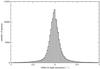 |
Fig. 1 Histogram of the off-sets between the quasars’ right ascension given in the original catalogue and those re-calculated through the LQRF algorithm. |
 |
Fig. 2 Histogram of the off-sets between the quasars’ declination given in the original catalogue and those re-calculated through the LQRF algorithm. |
To get a clear insight as to the differences brought by the recomputation of coordinates
we show in Figs. 1 and 2, respectively, the histograms of the off-sets in right ascension and
declination, between the quasar coordinates given in their original catalogue and those
recalculated through the LQRF algorithm. We note that both histograms present the same
Gaussian profile accompanied by a small asymmetry, with a slightly sharper aspect in
declination (Fig. 2) than in right ascension (Fig.
1). We took the factor cosδ into account to
evaluate the real angular offset in right ascension. The asymmetries mentioned above lead
to a relative global bias towards negative values in αcosδ and
positive ones in δ. Indeed, the mean values for both samples are
respectively  and
and
 , respectively, whereas the standard
deviations are
, respectively, whereas the standard
deviations are  and
and
 . The rather large amplitude of these
two last values attests to the generally poor astrometric quality of some of the original
catalogues involved in the LQAC-2 compilation and justifies the necessity to recalculate
them in the LQRF. We Note that they are of their order is the same as the positional
uncertainty of the UCAC-2 astrometric catalogue (Zacharias et al. 2004).
. The rather large amplitude of these
two last values attests to the generally poor astrometric quality of some of the original
catalogues involved in the LQAC-2 compilation and justifies the necessity to recalculate
them in the LQRF. We Note that they are of their order is the same as the positional
uncertainty of the UCAC-2 astrometric catalogue (Zacharias et al. 2004).
In a next paper, we plan to focus the present analysis on the sub-set of the 3414 objects of the ICRF2. It will be interesting, in particular, to check if the recalculated equatorial coordinates at optical wavelengths become closer to the ICRF2 coordinates obtained by VLBI than the original ones. Two supplementary remarks must be added: first a high proportion of ICRF2 objects have no optical counterpart either because of their faintness or because they has not been surveyed so far. Second, there is no insurance that optical photocentre of ICRF2 quasars correspond to the same position as that determined from VLBI. This is subject to recent investigations (Orosz & Frey 2013).
Difference of coordinates of quasars per V magnitude range, between the original catalogues of the LQAC-2 and the re-calculated values from the LQRF (Andrei et al. 2009).
2.2. Study of the magnitude dependence
As a supplementary study linked with astrometric performance, we investigated the
magnitude dependent systematic errors on the quasars’ positions. To this aim, we selected
all the quasars with an estimation of the V magnitude, which represents a sample of 91 183
objects (48.63% of the whole
LQAC-2). In Table 1, we list the mean values
 and
and  as well as the standard deviations σα ×
cosδ and σδ of the differences of
coordinates between those given by the original catalogues of the LQAC-2 and those based
on the improved values given by the LQRF recalculation, for each V magnitude bin. The
results for the standard deviations are plotted in Fig. 3 both in right ascension and declination. We can observe a very clear
correlation between the values of σα ×
cosδ and σδ, with a minimum at
as well as the standard deviations σα ×
cosδ and σδ of the differences of
coordinates between those given by the original catalogues of the LQAC-2 and those based
on the improved values given by the LQRF recalculation, for each V magnitude bin. The
results for the standard deviations are plotted in Fig. 3 both in right ascension and declination. We can observe a very clear
correlation between the values of σα ×
cosδ and σδ, with a minimum at
 and
and
 both for 18
<V<
19. The standard deviation is generally slightly smaller in declination
than in right ascension. Moreover, the general feature of the curves is in good agreement
with typical astrometric reductions, for which the best results in terms of accuracy are
obtained for intermediary values of magnitude. This is explained by saturation problems
for the brightest objects and insufficient S/N ratio for the faintest ones, both phenomena
leading to larger position errors.
both for 18
<V<
19. The standard deviation is generally slightly smaller in declination
than in right ascension. Moreover, the general feature of the curves is in good agreement
with typical astrometric reductions, for which the best results in terms of accuracy are
obtained for intermediary values of magnitude. This is explained by saturation problems
for the brightest objects and insufficient S/N ratio for the faintest ones, both phenomena
leading to larger position errors.
We have carried out exactly the same kind of study but with respect to the
g magnitude
instead of the V magnitude. This concerns 118 048 quasars, which
represent 62.96% of the whole
LQAC-2. Our results are presented in Table 2 and
plotted in Fig. 4. Here the values of the standard
deviation σδ are always
slightly smaller than σα ×
cosδ excepted for one magnitude bin considered,
with a minimum at  for 17
<g<
18 and
for 17
<g<
18 and  for 18
<g<
19. All these values, below
for 18
<g<
19. All these values, below  , are significantly smaller than in
the case of the precedent study by taking into account V magnitudes. This can be
explained by the following reason: quasars recorded with a V magnitude come from a
large set of individual catalogues, already compiled by Véron-Cetty & Véron (2010)
for most of them. They are characterized by poor astrometric quality, whereas quasars
recorded with a g magnitude come mainly from the SDSS catalogue (DR8
release) with homogenous and rather accurate astrometry. This explains that the agreement
with the LQRF optimized values of coordinates is much better. The astrometric quality in
g band is
stabilized at small values for a wide range of the g magnitude
(15
<g<
24) (Fig. 4), wheareas this
stability is not present in V magnitude (Fig. 3).
, are significantly smaller than in
the case of the precedent study by taking into account V magnitudes. This can be
explained by the following reason: quasars recorded with a V magnitude come from a
large set of individual catalogues, already compiled by Véron-Cetty & Véron (2010)
for most of them. They are characterized by poor astrometric quality, whereas quasars
recorded with a g magnitude come mainly from the SDSS catalogue (DR8
release) with homogenous and rather accurate astrometry. This explains that the agreement
with the LQRF optimized values of coordinates is much better. The astrometric quality in
g band is
stabilized at small values for a wide range of the g magnitude
(15
<g<
24) (Fig. 4), wheareas this
stability is not present in V magnitude (Fig. 3).
To complete our astrometric analysis, we plot the same kinds of histograms as for the
global set of LQAC-2 quasars of Figs. 1 and 2 with the sub-sets of quasars selectioned above, that is
to say, the 90 880 objects with V magnitude available (Figs. 5 and 6) and 118 048 objects with
g magnitude
available (Figs. 7 and 8). The sharpness of the histograms in the latter case with respect to the
former shows up obviously, both in right ascension (Figs. 5 and 7) and in declination (Figs. 6 and 8). This
sharpness is concretized by the corresponding values of the standard deviations:
 in g with respect to
 in V;
in V;
 in g with respect to
 in V. Concerning the mean
value of the coordinates off-sets, we note in both cases a negative bias in right
ascension with
in V. Concerning the mean
value of the coordinates off-sets, we note in both cases a negative bias in right
ascension with  in g and
 in V; The bias is close to
zero with
in V; The bias is close to
zero with  in g and
 in V for the declination.
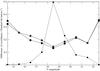 |
Fig. 3 Standard deviation between the quasar coordinates given in the original catalogue and those re-calculated through the LQRF algorithm, with respect to V magnitude. Right ascension (upper curve) and declination (lower one). The dashed line indicates the normalized number of quasars. |
 |
Fig. 4 Standard deviation between the quasar coordinates given in the original catalogue and those re-calculated through the LQRF algorithm, with respect to g magnitude. Right ascension (upper curve) and declination (lower one). The dashed curve indicates the normalized number of quasars. |
 |
Fig. 5 Histogram of off-sets in right ascension between the quasar coordinate given in the original catalogue and the one recalculated through the LQRF algorithm. The quasars considered are restricted to those that present an estimation of V magnitude. |
 |
Fig. 6 Histogram of off-sets in declination between the quasar coordinate given in the original catalogue and the one re-calculated through the LQRF algorithm. The quasars considered are restricted to those that present an estimation of V magnitude. |
3. The whole sky lack of homogeneity in the distribution of recorded quasars
Two main reasons lead to the lack of uniformity of the surface distribution of the quasars already discovered and recorded on the celestial sphere. The first one must be considered as an observational defect: it comes from the fact that each survey participating in a compiled catalogue, such as the LQAC-2 (Souchay et al. 2012), is more or less dense and complete at a given threshold of magnitude and covers a limited and generally relatively small area in the sky. Therefore the combination of the catalogues involved is naturally a source of large inhomogeneities in terms of surface density on the celestial sphere, including depletion zones for which no systematic or extended survey has been achieved so far.
The second reason is physical. It arises from the galactic extinction, which is all the more important that we consider fields close to the galactic plane, that is to say, with small absolute values of the galactic latitude. In the following, we study, with the help of histograms, the variations of surface density of the recorded quasars in the LQAC-2, with respect to galactic, equatorial, and ecliptic coordinates.
3.1. Galactic coordinates distribution
In Figs. 9 and 10 we show the histograms of the population distribution of the LQAC-2 quasars as a function of the galactic longitude l and the galactic latitude b, respectively. The horizontal line in Fig. 9 and the rounded one in Fig. 10 show the features that should be followed by these histograms in the ideal case of a uniform surface distribution. The impact of the galactic extinction on the drastic decrease of the number of objects for low absolute values of b is clearly seen in Fig. 10. For − 10°<b< + 10°, the number of recorded quasars is around 1000 objects per bin whereas it should reach approximately more than 16 times this value in the case of a homogeneous distribution. We must emphasize that this ratio should be even much larger if we only take the optical sources into account and exclude the radio emitting sources that are poorly affected by the galactic extinction. The ratio of the number of quasars in the northern galactic hemisphere to those in the southern hemisphere, which is equal to 2.614, is largely explained by the discrepancy between the surveys in the respective hemispheres, also noticed for the equatorial coordinates, as will be pointed out in the following.
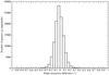 |
Fig. 7 Histogram of off-sets in right ascension between the quasar coordinate given in the original catalogue and the one re-calculated through the LQRF algorithm. The quasars considered are restricted to those that present an estimation of g magnitude. |
 |
Fig. 8 Histogram of off-sets in declination between the quasar coordinate given in the original catalogue and the one re-calculated through the LQRF algorithm. The quasars considered are restricted to those that present an estimation of g magnitude. |
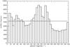 |
Fig. 9 Histogram of the quasar population with respect to galactic longitude. The straight line represents the shape the histogram should have in the case of a homogeneous distribution. |
 |
Fig. 10 Histogram of the quasar population with respect to galactic latitude. The curved line represents the shape the histogram should have in the case of a homogeneous distribution. |
3.2. Equatorial coordinates distribution
A dense and homogeneous space distribution of the equatorial coordinates of quasars is desirable for a reference frame. Indeed, quasars play the fundamental role as quasi-inertial reference objects, as has been demonstrated in the construction of the ICRF (Ma et al. 1998) and its up-dated version the ICRF-2 (Ma et al. 2009) built from observations carried out with the VLBI technique at radio wavelengths. With the event of the Gaia astrometric space mission launched December 19 2013 from the Guyana Space Center, optical observations are expected to be the key for the construction of a very dense and accurate celestial reference frame at optical wavelengths in the near future, maybe at the end of the decade. For this purpose, a rather uniform distribution in the celestial sphere in terms of equatorial coodinates is greatly recommended.
Although Gaia should considerably improve both surface density and uniformity of recorded quasars, it is instructive to study these topics with the present available sample. Thus, this sub-section is devoted to the analysis of the present quasars distribution inside the LQAC-2 compiled catalogue with respect to the equatorial coordinates. In Figs. 11 and 12, we show the histograms of the distribution of quasars of the LQAC-2 in right ascension and declination, respectively, with 10° (40mn) bins. In declination (Fig. 12), there is a general depletion of quasars in the southern hemisphere and in opposite a large excedentary count in the northern hemisphere, with respect to a uniform distibution represented by the rounded curve. This is obviously because, by far, the largest survey, the SDSS, which contains 67.51% of the total sample of the LQAC-2 (187 504 quasars), is concentrated in the northern hemisphere. Only 14 176 objects among the 126 577 ones representing the whole SDSS population belong to the southern hemisphere, that is to say a mere 11.20%. If we consider the whole LQAC-2 catalogue, the counts are 51 887 (27.67%) and 135 617 quasars (72.33%) respectively in the southern and northern hemispheres. Here two gaps appear neatly in right ascension (Fig. 11) centred around 90° and 290°, respectively, with no explanation other than the lack of uniformity of surveys.
 |
Fig. 11 Histogram of the quasar population with respect to right ascension. The straight line represents the shape the histogram should have in the case of a homogeneous distribution. |
 |
Fig. 12 Histogram of the quasar population with respect to declination. The curved line represents the shape the histogram should have in the case of a homogeneous distribution. |
3.3. Ecliptic coordinates distribution
The ecliptic band (− 30°<β< + 30°) being the priviligiate zone in which the overwhelming majority of moving objects (planets, asteroids, etc.) are detected and monitored, it also looks interesting to investigate the surface density of quasars through this band. Indeed, we can expect that, in the near future, following the Gaia mission output data, a large number of astrometric reductions of these moving bodies will be carried out directly from quasars instead of stars, on the condition that the sky surface density of the former objects is large enough. This issue has already been studied by Souchay et al. (2007) when searching for the cases of close approaches between quasars and Jupiter with possible applications to the Gaia mission. An underlying purpose in that particular study of the biggest planet was to estimate theoretically the relativistic deflection of light due to its gravitation.
In Figs. 13 and 14, we present the histograms of a number of LQAC-2 objects with respect to their ecliptic longitude and ecliptic latitude. As mentioned in the preceding subsection for equatorial coordinates, and because of the small inclination (23°27′) of the ecliptic with respect to the celestial equator, we observe (Fig. 14) a dramatic excess of quasars in the part corresponding to positive ecliptic latitudes with respect to negative ones, which is essentially a consequence of a much extended coverage of sky observations in the northern hemisphere, Here also the two gaps in ecliptic longitude appear clearly in Fig. 13, correlated with those already observed in right ascension (Fig. 11).
 |
Fig. 13 Histogram of the quasar population with respect to ecliptic longitude. The straight line represents the shape the histogram should have in the case of a homogeneous distribution. |
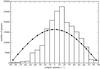 |
Fig. 14 Histogram of the quasar population with respect to ecliptic latitude. The curved line represents the shape the histogram should have in the case of a homogeneous distribution. |
4. Distance to the nearest neighbour: statistical analysis
In the case of a compiled catalogue, such as the LQAC-2, the distance to the nearest neighbour, or by extension to the kth neighbour is a fundamental parameter that should naturally obey some statistical law in the case of a uniform distribution. A general theoretical overview of the topic can be found in a Gaia DPAC Technical Note by Mignard (2008). In the following, we recapitulate the main steps of the theory to confront it with the real quasars sample of the LQAC-2.
4.1. Theoretical calculations and expected results
When supposing a point Q of the celestial sphere located at the centre of a
circular area S =
πr2, let ρ be the surface density,
so that λ =
ρS represent the mean number of sources expected in
S. In a
homogeneous sources repartition, the probability P(k) that
there are exactly k points, (k = 0,1,2...) in
S is given
by a Poisson distribution:  (1)As a consequence,
the probability that no source is found in an S is:
(1)As a consequence,
the probability that no source is found in an S is:
 (2)Thus, the
probabilty that at least one source is present inside S, that is to say, that the
distance d to
the nearest neighbour is smaller than r, is:
(2)Thus, the
probabilty that at least one source is present inside S, that is to say, that the
distance d to
the nearest neighbour is smaller than r, is:
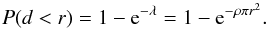 (3)From this last
equation, we get by derivation the probability density function (PDF) for the angular
variable r:
(3)From this last
equation, we get by derivation the probability density function (PDF) for the angular
variable r:
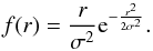 (4)Where σ can be introduced as a
characteristic distance, that is to say the average distance to find the nearest neigbour:
(4)Where σ can be introduced as a
characteristic distance, that is to say the average distance to find the nearest neigbour:
 (5)These theoretical
calculations can be extended to the search for the kth nearest neigbour
(Mignard 2008). Then the smallest distance
corresponds to the nearest neighbour, the second smallest to the second nearest neighbour,
etc. until the kth distance. The corresponding formula for PDF of
the kth
nearest neighbour, can be written:
(5)These theoretical
calculations can be extended to the search for the kth nearest neigbour
(Mignard 2008). Then the smallest distance
corresponds to the nearest neighbour, the second smallest to the second nearest neighbour,
etc. until the kth distance. The corresponding formula for PDF of
the kth
nearest neighbour, can be written:  (6)In the following, we only
deal with the study of the nearest neighbour, concerning the LQAC-2.
(6)In the following, we only
deal with the study of the nearest neighbour, concerning the LQAC-2.
 |
Fig. 15 Histogram of the number of quasars with respect to their distance to the nearest neighbour in the whole LQAC-2 catalogue. The line shows the shape the histogram should have according to the theory, if uniform distribution is assumed. |
4.2. Comparison with the all-sky LQAC-2 catalogue and a large SDSS survey field
In this sub-section, we confront the theoretical results presented above with real
samples of quasars. At first, we take the whole LQAC-2 quasars population, containing
187 504 objects distributed in the whole celestial sphere. This concerns an all-sky
surface area of 41 253 square degrees, which gives a density ρ = 4.545 sources per
square degree. Using (3), the probability that the distance between a quasar and its
nearest neighbour is located between two consecutive radii values r1 and
r2 is:
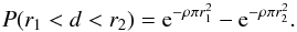 (7)Multiplying this
probability by the total number of quasars in the sample considered, we can compare our
theoretical expectation with the histogram of the number of sources with respect to the
value of the closest distance. This comparison is shown in Fig. 15. We observe that the theoretical curve corresponding to a typical
Rayleigh distribution does not fit the results at all. This can be easily understood as
the consequence of a lack of homogeneity of the sample in the celestial sphere. Because of
the high density of quasars due essentially to the SDSS survey in some area covering
roughly 1/3 of the sky, the peak for the largest number of quasars is reached near
d =
200′′ whereas its theoretical value is close to
d =
700′′. We oberve a drastic depletion of quasars for values
of the angular distance in the interval 600′′<d<
2000′′, which is clearly attributable to the fact that
when we exclude the large and dense surveys participating in the present known quasar
population, the quasars surface density is excessively small in some zones of the
celestial sphere.
(7)Multiplying this
probability by the total number of quasars in the sample considered, we can compare our
theoretical expectation with the histogram of the number of sources with respect to the
value of the closest distance. This comparison is shown in Fig. 15. We observe that the theoretical curve corresponding to a typical
Rayleigh distribution does not fit the results at all. This can be easily understood as
the consequence of a lack of homogeneity of the sample in the celestial sphere. Because of
the high density of quasars due essentially to the SDSS survey in some area covering
roughly 1/3 of the sky, the peak for the largest number of quasars is reached near
d =
200′′ whereas its theoretical value is close to
d =
700′′. We oberve a drastic depletion of quasars for values
of the angular distance in the interval 600′′<d<
2000′′, which is clearly attributable to the fact that
when we exclude the large and dense surveys participating in the present known quasar
population, the quasars surface density is excessively small in some zones of the
celestial sphere.
To avoid this artefact because of the lack of uniformity and to find a better agreement with theoretical expectations, we must carry out our study in a limited and homogeneous area of the sky, that is to say, with a relatively constant surface density. We naturally choose a zone of the LQAC-2 covered by the SDSS, but also containing objects from other catalogues. It is limited by the following conditions: 8h40m<α< 16h and 5°<δ< 55°. Indeed, in this new case, the histogram presented in Fig. 16 fits the theoretical estimation well: the real distribution of the sample with respect to the distance of the nearest neighbour is in good agreement with the theoretical curve, and it peaks for a value in accordance with the characteristic distance of σ = 375′′. Nevertheless, with a meticulous and more detailed inspection, we note that the correspondence between our sample and the theory is not perfect: there is a small O−C discrepancy characterized by an excedent of the true distribution of quasars for nearly all the values of d<σ and a significant deficiency of the number of quasars for the values of distance σ<d< 800′′. This can be attributable to an effect of the remaining imperfection in homogeneity of the quasars distribution in the area selected, because we took catalogues other than the sole SDSS into account.
A more careful and deeper analysis of the small discrepancy mentioned above could be performed by investigating the density variations inside sub-zones of the sample. These densities could have different causes such as a real inhomogeneity in the quasar’s distribution, biases due to observational climatic conditions (seeing), or declination effects. This analysis is out the scope of this paper. Here we simply want to emphasize the good correlation between the histogram of the distribution with the basic theoretical distribution law.
 |
Fig. 16 Histogram of the number of quasars with respect to their distance to the nearest neighbour in a specific zone of the LQAC-2 with homogenous surface density. The line shows the shape the histogram should have according to the theory, if uniform distribution is assumed. |
4.3. Uncertainties for quasars pairing at short angular distance
Following the study above, we take a particular here care to the excedent of quasars characterized by short angular distances to the nearest neighbour, i.e., with small values of d. Figure 17 represents a zoom of the histogram in Fig. 16 for 0°<d< 200′′. We note a significant excess of quasars in the histogram at very small distance (d< 30′′) with respect to the theoretical curve. This deserves specific attention because this excess should have different origins. Indeed, admitting that the theoretical curve represents cases of hazardous coincidence between two quasars in nearly the same line of sight, the excedent should be explained by two kinds of external cases. First, it should come from the presence of double listings in the LQAC-2 catalogue, that is to say, of a single object which, by a failed cross-identification, has been recorded twice with different coordinates. Second, it should have a physical origin and cosmological relevance: we are in presence either of a true case of binary quasars, linked by gravitational interaction, or of gravitational lensing of a single quasar reproduced twice.
The redshift related to the two objects is expected to be roughly the same, whether a double listing or a true binary. Thus, the redshift comparison is not suitable to separate the two external cases above. But such a comparison can, at least, differentiate couples of quasars in excedent from those predicted by the theory, as we explained above, for which a significant z difference between two paired quasars a priori validates the thesis of the presence of two real coincident objects with no physical interaction.
In Fig. 18, we represent in a bi-dimensional (z1,z2) graph the couple of quasars for which d< 10′′. The redshift of a quasar considered is z1 and z2 the nearest neighbour’s redshift. Frequently, a point has a symmetric with respect to the first diagonal, because, most of the time, the first quasar in a couple quasar/nearest neighbour is also the nearest neighbour of the second one (but not all the time, we will see an example in Table 4). A zone is delimited by two parallel lines following this condition: the number of points (z1,z2) inside this zone is equal to the excedent of couples of quasars from theoretical expectations, and so the number of points (z1,z2) outside this zone represents the expected cases of hazardous coincidences, in other words, quasars close to each other but with no equal redshift.
 |
Fig. 17 Zoom at the shortest distances d of the histogram in Fig. 16. The line shows the shape the histogram should have according to the theory. |
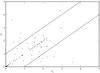 |
Fig. 18 Position of couples quasar/nearest neighbour in a bi-dimensional (z1,z2) graph in the case of quasars with an angular separation shorter than 10 arcsec. |
The same process is applied to the next bins in the histogram, that is to say, 10′′<d< 20′′ in Fig. 19 and 20′′<d< 30′′ in Fig. 20. The results can be considered as convincing if and only if the zone between the two parallels is restricted to the first diagonal and its surroundings. As we can see in Figs. 19 and 20, we cannot separate the two parallel lines with naked eye, which is because quasars in the zone delimited by these two lines have a difference in redshift of less than 0.1. So the excedent can be explained by physical couples of quasars or double listings. In Fig. 18, we remark that the two lines are far away from the other and the ends of the zone reach a difference in redshift of close to 1. In conclusion, for 10′′<d< 30′′, the excedent estimated between the theory and the real sample of the LQAC-2 can be explained by physical pairs of quasars (or single quasar seen under gravitational lensing) and double listings, but at the closest distance (d< 10′′) physical quasars and double listings are not enough to explain an excedent. This contradicting result is difficult to interpretate.
4.4. Identification and confirmation of binary quasars
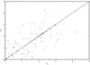 |
Fig. 19 Position of couples quasar/nearest neighbour in a bi-dimensional (z1,z2) graph in the case of quasars with an angular separation between 10 arcsec and 20 arcsec. |
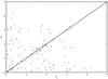 |
Fig. 20 Position of couples quasar/nearest neighbour in a bi-dimensional (z1,z2) graph in the case of quasars with an angular separation between 20 arcsec and 30 arcsec. |
In the continuity of the study above, the search for binary quasars looks like an interesting by-product of huge surveys. For instance, Hennawi et al. (2006) presented a sample of 221 quasar pairs, over the redshift range 0.5 <z< 3.0, discovered from an extensive follow-up campaign to find companions around the SDSS and 2dF QSO surveys. In particular, this sample includes 26 new binary quasars with separation θ< 10′′, which corresponds to proper transverse separation Rprop< 50 h-1 kpc.
Following our investigation above we wanted to characterize real binary quasars. To that
end, we identify the pairs of quasars with a redshift difference smaller than
 ,
where Δz0 is an arbitrary threshold. The factor
,
where Δz0 is an arbitrary threshold. The factor
 comes from the fact that we work with the distance to the first diagonal of a couple
(z1,z2)
given by the expression
comes from the fact that we work with the distance to the first diagonal of a couple
(z1,z2)
given by the expression  .
In our study, we adopt Δz0 = 0.02, which looks reasonable when
considering the precision of redshift determination (Souchay et al. 2009).
.
In our study, we adopt Δz0 = 0.02, which looks reasonable when
considering the precision of redshift determination (Souchay et al. 2009).
So, as double listings and true double quasars present the same redshift at this level, the only possibility to make an adequate differentiation between these two categories consists in searching deep field images of these objects. We decided to rely on SDSS images, when available, at the following site: http://cas.sdss.org/astro/en/tools/search/IQS.asp. Our selection for the search and validation of binary quasars leads to a set of 289 pairs based on the following constraints: their angular distance must be d< 30′′ and their off-set Δz with respect to the line z1 = z2 should be less than Δz0 = 0.02. For this global set we found 159 real binary quasars (with three of them doubtful), i.e., with same redshift and two photocentres, and 35 double listings (with five of them doubtful), for which there is only one photocentre visible on the frame. Nevertheless, in this last case we cannot exclude the possibility that we are in the presence of a real binary quasar for which one of the photocentres is out of detection from the DSS image database. At last, 97 pairs could not be accessible to the DSS data and are still waiting for further observational investigation. The fact that double listings exist at an angular distance of several arcseconds is not surprising. Some original quasars catalogues belonging to the LQAC-2 compilation present a poor positional accuracy at this level. They are not concerned by the analysis presented in Sect. 2.1 for they were not identified by the LQRF algorithm because of their poor astrometry.
We recognize that the present study constitutes a preliminary effort in the identification of binary quasars. Some point can be deepened, for example the definition of the limit of redshift difference between two quasars to consider them as binary quasars. Nevertheless, we think that this kind of analysis should be deepened at least to evaluate the proportion of binaries objects among the total sample of known quasars statistically.
An important remark, from a private communication (Mignard 2013) based on personal investigations, was that the probability that a quasar undergoes a gravitational lensing should be about 1 / 1000. So it looks legitimate to require further analysis and to understand at what extent our set of binary quasars should or should not be the consequence of these lensings. We observe that the number of binary quasars we found (159) corresponds to a little less than one thousandth of all the 187 504 quasars in the LQAC-2 catalogue. In fact, the possibility that quasars clustering at short angular distances (2′′< Δθ< 10′′) are due to gravitational lensing has been abundantly investigated for more than a decade, with the conclusion that the expected number of quasars lensed by groups and clusters is too small to account for all the controversial pairs (Oguri & Keeton 2004; Hennawi et al. 2007). The plausible explanation is that the controversial pairs are real binaries rather than lenses (Schneider 1993; Kochanek et al. 1999; Mortlock et al. 1999). Djorgovski et al. (1991) as well as Hewett et al. (1998) similarly claimed that this interpretation implied a factor 100 more binary quasars over what is expected from extrapolating the quasar correlation function power law down to co-moving scales smaller than 100 h-1 kpc. The first work interpretated this fact as the enhancement of quasar activity during merger events. The estimation of the factor above was done before the advent of very dense surveys as the 2dF and the SDSS, and should be re-calculated by taking their statistics into account.
Binary quasars of the LQAC-2 with the highest redshifts.
Binary quasars with the lowest redshifts (two of them form a triplet).
4.5. Examples of interesting binary quasars
This sub-section is devoted to a sub-sample of physical binary quasars with exceptional characteristics coming from the total LQAC-2 compilation. They should present some interest because of their uncommon properties. We have carefully checked the binary status of all of them via the DSS imaging database. In Tables 3 and 4, we show quasar binaries with the highest and lowest redshift value, respectively, whereas, in Table 5, we show binaries whose one of the component is among the brightest ones in U band. Finally, in Table 6, we selected binaries with the smallest angular separation. In all these tables, for the sake of concision, the quasars are referenced from their LQAC number instead of their equatorial coordinates. Moreover, we give all the relevant information when it is available: the angular separation r, the redshift z, and the U magnitude. For each binary component we mention the LQAC-2 flag indicating the original catalogue from which it has been picked up (Souchay et al. 2012). In all our tables we limitated our search for binaries within a maximum separation θ = 30′′.
Binary quasars with the brightest magnitude U for one of their components.
Binary quasars with the smallest separation.
Binary quasars with the shortest separation, between 0′′ and 30′′.
Some interesting remarks can be driven from these sub-samples. First, in Table 3, where we list the binary quasars with the highest redshift, we find a pair with z> 3 despite the fact that the population in this area is relatively very small as will be shown in Sect. 5.4. The following very distant binaries have a redshift around z = 2.5. On the other hand, in the case of binaries with the smallest redshifts (see Table 4), the values of these redshifts are z< 0.1. As could be expected some of the binaries with brightest component in Table 5 are also included in Table 4 with the lowest redshift. But some quasars do not follow this rule, as in the case of Lqac_137+000_026 with a redshift of 1.873 despite a relatively bright component at U = 16.9, making it the fifth brightest binary.
In Table 6, we observe that the nine closest binaries have an angular separation between 2′′ and 3′′. As a complement we present in Table 7 the complete list of the 159 binary quasars that we have clearly identified from DSS imaging, with a separation angle θ between 2′′ and 30.̋. The objects are arranged in order of increasing θ. The U magnitudes of the two components are indicated (when available) as well as their redshift, the flag of the catalogues in which each component can be found, and a number indicating the sequential number in terms of increasing magnitude U of the brightest component and decreasing value of z. We think that this extended list will be profitable for further purpose, for instance dissociating the cases of true binaries from those of gravitational lensing by specific spectral characterization. In many cases the SDSS survey (flag “E”) has identified only one of the two components despite their relative proximity.
5. Cross-identification and cross analysis of two surveys in high density fields: SDSS and 2dF
A particular and interesting study concerns the inter-comparison between two independent dense catalogues on a common explored sky area. Some important issues can be adressed from it. For instance, for the selected area, we can investigate, at a given magnitude threshold, the number of quasars common in the two surveys as well as those detected in only one survey. Thus, we can evaluate the level of completness of the respective catalogues, which could be dependent on the method of detection of the objects.
Two catalogues are particularly suitable for our study, because they are both relatively very dense and contain a rather extended common surveyed sky area: the Sloan Digital Sky Survey (SDSS, Adelman-Mc.Carthy et al. 2007) and the 2-degree Field Quasar Redshift Survey (2dF, Croom et al. 2004). After describing the properties of these surveys as well as their specific underlying method of detection of quasars, we show the results of the analysis coming from their cross-identification.
5.1. The characteristics of the SDSS and the 2dF surveys
The Sloan Digital Sky Survey, generally referred as SDSS, results from observations performed with a dedicated 2.5 m telescope at Apache Point (New Mexico, USA). The pre-selection of the quasars is based on analysis the u, g, r, i, z photometric database of the catalogue and on the analysis of the colour indexes (u − g, g − r, r − i, i − z) which are significantly different from normal stars. Once a candidate has been detected, its spectrum is obtained and the detection of broad emission lines, characteristic of a quasar, is validated from an automated analysis pipeline. A specific software detects absorption and emission lines, and fits a Gaussian function to each line profile. The SDSS criteria to qualify an object as a quasar is that at least one line must have a full-width at half maximum (FWHM) broader than 1000 km s-1. Moreover, an additional condition is that the object must be intrinsically brighter than Mi = −22.
Similar to the SDSS, the 2-degree Field (2dF) Quasar Redshift Survey, quoted as 2QZ (Croom et al. 2004) is based on a pre-selection of quasar candidates using well defined criteria on three u, b, r colours (instead of five for the SDSS). Nevertheless, the support is fundamentally different for it consists of automated measurements of UKST photographic plates. As in the case of the SDSS, a spectroscopic follow-up of the candidate quasars is completed, using a χ2 minimization technique to fit the spectrum to a number of quasars, galaxies, and stellar templates.
5.2. Cross-identification between the two surveys in a large common field
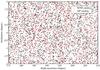 |
Fig. 21 Mapping of quasars present both in catalogues SDSS and 2dF. The area is restricted to the common area of those two catalogs and presented in equatorial coordinates. |
In order to estimate the relative completeness of the two surveys above and to identify the differences between them concerning information on the quasars taken individually, we choose a fully explored common sky area. It corresponds to an area delimited by the following equatorial coordinates intervals: 11h40m<α< 14h and − 2°<δ< + 2°.
This area, shown in Fig. 21 contains 4326 quasars among the 23 660 included in the 2dF catalogue, that is to say, 18.28% of the sample, and 1731 quasars among the 126 577 of the SDSS (8th release), which corresponds to 1.36%. A cross-identification in the area above leads to a surprising result: this area totals 5157 quasars present in at least one of the two surveys, but with only 900 objects belonging to the two catalogues (17.55%), 831 only to the SDSS (16.20%) and 3426 only to the 2dF (6682%).
Moreover, to the set of 5157 quasars mentioned above we must add 2563 quasars belonging neither to the SDSS nor the 2dF to the set of 5157 quasars mentioned above. They are present in the selected area and included in the LQAC-2. Half of them come from various sub-catalogues already compiled by Véron-Cetty & Véron (2010). The other half comes essentially from a specific investigation of the common area by da Angela et al. (2008). Thus, the total number of quasars discovered in the area amounts to 7720 objects. With respect to this total number, the percentages above are significantly reduced: no more than 22.42% of objects have been detected by the SDSS, 55.14% by the 2dF and only 11.65% by both surveys. Last, a substantial percentage of 33.20% of objects have not been detected in at least one of the two main surveys.
 |
Fig. 22 Histogram of quasars in the common area of the SDSS and the 2dF with respect to their R magnitude. We present quasars in different curves, depending on if they are common to both catalogues, and therefore depending on which catalogue the value of the magnitude comes from, or if they are present in only one catalogue. |
This means that the SDSS, which is the most ambitious quasar survey ever produced, and which gives an essential part of its objects to the LQAC-2 (67.51%), misses a majority of them (roughly about 3/4) in a given explored area. This fact should not be attributable to the limiting magnitude of detection of the SDSS survey, which is much larger than in other surveys, as will be detailed below. In comparison, the 2dF, which concerns a rather limited area of the sky, can be considered as a particularly meticulous and efficient survey, with roughly 2.5 more quasar detections for a same explored area. In conclusion, we can assert that these two surveys leave a significant large quantity of discoveries to be made, not only in the southern hemisphere, which has been poorly investigated so far, but also in the northern hemisphere, even for areas already explored.
5.3. Photometric comparative analysis
To deepen the comparative study between the two catalogues and to understand the reasons of the relatively poor number of common quasars better, we have performed a photometric analysis of the objects present in both of them. In Figs. 22 and 23, we present the histograms, with respect to respectively the R and U magnitudes, of the objects detected in at least one of the two surveys. In particular, we separate the cases for which the quasar is common to the two catalogues or not and, for cross-identified quasars, we indicate where the value of R or U magnitude comes from. The U and R magnitudes coming from the SDSS and 2dF do not exactly refer to the same nominal wavelengths and bandwidths. In the case of the SDSS (Gunn et al. 1998), the U band (noted u) corresponds to λeff = 0.3549 μm and a FWHM = 0.0560 μm whereas information cannot be extracted easily concerning the 2dF survey (Croom et al. 2004; Lewis et al. 2002).
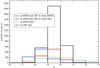 |
Fig. 23 Histogram of quasars in the common area of the SDSS and the 2dF with respect to their U magnitude. We present quasars in different curves, depending on if they are common to both catalogues, and therefore depending on which catalogue the value of the magnitude comes from, or if they are present in only one catalogue. |
In the R band (Fig. 22), we can observe that the peak of common quasars ranges between 18 <R< 19, whereas the overwhelming majority of quasars detected by the sole 2dF corresponds to 19 <R< 21. The relative number of quasars detected per magnitude bin is comparatively much more contrasted for the 2dF than for the SDSS. Thus, we remark that the number of objects detected by the 2dF alone is nearly the same as the number of objects detected by the SDSS alone for 18 <R< 19, whereas this number is roughly seven times larger for the following bin (19 <R< 20) and even ten times larger for 20 <R< 21. Last the origin of the R magnitude estimation (SDSS or 2dF) does not influence significantly the histogram for quasars common to the two catalogues. The parameter R = 22 represents roughly the limit of the detection (Fig. 22).
In the U band (Fig. 23) the origin of the magnitude value significantly influences the statistics for common quasars. When U (in fact u) is taken from the SDSS, the peak number of common identifications arises for 19 <u< 20 whereas it corresponds to 18 <U< 19 when it is taken from the 2dF. Here the very large majority of detections by the 2dF alone occurs for 18 <U< 21, with a very neat peak for the central bin, for which the number of detections is more than 10 times the corresponding one by the SDSS alone. This ratio falls to slightly greater than 3 for the following bin (20 <R< 21). In comparison, for the SDSS, the magnitude interval for a significant number of detections is much bigger, ranging between u = 17 and u = 25. Finally, the number of quasars present in 2dF but not in the SDSS as well as in contrast the number of quasars present in SDSS but not in 2dF peak at the same R or U magnitude bin (19 <R or U< 20). From all these results we can conclude that the relatively small number of cross-identifications between the two surveys is explained in a large part by different detection sensitivities with respect to magnitude intervals.
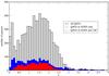 |
Fig. 24 Histogram of the number of SDSS quasars with respect to z. In red, proportion of quasars common to the SDSS and 2dF surveys; in blue, quasars only in SDSS catalogue; in grey, quasars missing from SDSS and 2dF. |
 |
Fig. 25 Histogram of the number of 2dF quasars with respect to z. In red, proportion of quasars common to the SDSS and 2dF surveys; in green, quasars only in 2dF catalogue; in grey, quasars missing from SDSS and 2dF. |
 |
Fig. 26 Value of the standard deviation of zSDSS − z2dF for quasars common to SDSS and 2dF surveys. |
5.4. Redshift comparative analysis
To complete our study, and to fully benefit from the presence of the common 2dF-SDSS selected area, we focus on the redshift of quasars present or missing in both surveys. The histograms of the number of quasars with respect to their redshift are presented in Figs. 24 and 25, respectively, for the SDSS and for the 2dF. For the sake of comparison, we also present in each figure the histogram of quasars common to the two surveys as well as the histogram of the total sample of recorded quasars in the explored area. Some important remarks can be pointed out. First, for very low redshifts (z< 0.2), the contribution of both large surveys is very small with respect to that of other catalogues. This is certainly due to selection effects, wherein the photometric filtering algorithms lead to particularly efficient selection of candidate quasars, in both surveys, for sufficiently large values of z.
Second, all the histograms present a leading peak around z = 1.5. By combining the QSO sample from the 2dF-SDSS luminous red galaxy (LRG) and QSO survey, da Angela et al. (2008) remarked on and deeply investigated the clustering of z ≈ 1,5 QSO’s, deducing some cosmological consequences from appropriate correlation functions.
Third, the histogram for quasars only detected by the SDSS is rather flat with a short peak for a small redshift value (at z = 0.3), which can again be explained by a selection effect. At last, the cut-off limit for z in the 2dF survey as well as for the other surveys, except the SDSS, is around z = 3, whereas for this last catalogue a significant number of quasars is found up to z = 5. Detections of objects with 5 <z< 7 are not represented because of their very small relative number. Whatever is considered to be the z interval, the number of quasars detected by the SDSS alone (24) is slightly bigger than the number of quasars in common, whereas it is several times larger in the case of the 2dF (Fig. 25).
Another instructive topic related to the common selected area concerns the comparison of the values of the redshifts for the cross-identified quasars in both surveys. This gives clear and direct information on the external accuracy of the z determination and its dependency on the value of z itself. In Fig. 26, we show the standard deviation between the determinations of z done by each survey, with respect to each 0.1 interval of z. We can notice that the difference is smaller than 0.04 excepted for two intervals for which the number of objects is particularly high, i.e., 1.5 <z< 1.6 and 1.8 <z< 1.9, respectively. Finally, the quality of determination is much better for z< 1 with an uncertainty smaller than 0.02, than for z> 1, where it is generally larger than this last value.
6. An estimation of the whole set of quasars NGaia detectable by the space probe Gaia
The results shown in the preceding section should help us to make a rough evaluation of the total number of quasars NGaia that could be detected by the space astrometric mission Gaia. To understand the method of detection of quasars by the probe we can refer to Mignard (2002): the major problem will be the recognition among many point-like sources, as stars. Several indicators will help make the decision, such as the absence of parallax, the negligible proper motion, the short term variability and, before all, the spectral signature summarized by a set of colour indices. Indeed, the combination of the broadband and medium band filters will permit a photometric identification of quasars from virtually any type of star. In particular, the decontamination from white dwarfs, a traditional contaminant in colour selected quasars will be resolved from medium band colours thanks to a good sensitivity to the Lyα line. In the following, we accept the principle that from these criteria that the quasars as selected by Gaia will be the same kinds of objects as those compiled in the LQAC-2.
As the detection of quasars by the satellite will be possible under the magnitude threshold V = 20 (Mignard 2002), NGaia could be determined from the following principle: first, we estimate the total number of quasars with V< 20 in the dense area considered in the last section, common to the SDSS and 2dF surveys. Second, we simply extrapolate this number to the whole sky. Third, we take the galactic extinction into account, which significantly diminishes the value of NGaia. This way of computation is rather straightforward once we have solve two difficulties. First, we have V magnitudes for only 3775 quasars in the selected area, which constitutes no more than 48.90% of the total population of 7720 recorded objects, whereas the U magnitude has been evaluated for a large majority of 7662 objects, that is to say, 99.25% of the sample. Second, it is difficult to evaluate the ratio ρG.E. of the number of quasars non-visible because of the galactic extinction, which concerns a band of galactic latitude included roughly inside the interval −20°<b< + 20° (Fig. 10).
We can remedy the first difficulty by adopting the following procedure: for the 3749 quasars of the selected area having both a V and a u magnitude we calculate at a given magnitude m (and more particularly for m = 20) the ratio of quasars with V<m to the number of quasars with u<m. The results are shown in Fig. 27 for each integer value of the magnitude between m = 15 and m = 23.
 |
Fig. 27 Numbers nV and nU of quasars found at a given magnitude threshold in a dense selected sky area, respectively in V and U bands. The thin curve indicates the ratio nU/nV. (This ratio is multiplied by 1000.) |
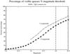 |
Fig. 28 Percentage of quasars found at a given magnitude threshold in a dense selected sky area, in V and U bands, respectively, with respect to the total number of qusars detected. The dashed vertical line corresponds to the GAIA cut-off in V band. |
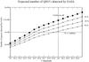 |
Fig. 29 Number of expected quasars detected by the GAIA satellite during its mission, according to four values of the percentage of quasars missed because of the galactic extinction missing ratio ρG.E. = 0,0.1,0.2,0.3. |
We study the value of the ratio in a magnitude range that concerns us particularly, around the Gaia V magnitude cut-off, between 19.0 and 20.5. This ratio, always bigger than 1, is slightly decreasing with the magnitude. It takes the maximum value 1.583 for V = u = 19.0, and the minimum value 1.113 for V = u = 20.4. Then, we extrapolate this ratio to the total sample of 7720 quasars detected in the area. This gives us an estimation of the total number of quasars visible at a given V magnitude threshold. At the magnitude value m = 20.0, the ratio V/u of quasars visible below this threshold is 1.140. Supposing that the sample of 4283 quasars (55.9%) detected in the area and characterized by u< 20.0 represents the complete estimation, we deduce that approximatively 4882 quasars should be visible at V< 20.0 for the same area, which corresponds to 63.7% of our sample. By adopting the same process we could deduce the ratio of quasars visible in the field at various magnitude thresholds from 18 <u< 20.5 and 19 <V< 20.5. The results are presented in Fig. 28 with the real percentages for u and the extrapolated ones for V, with respect to the total sample.
Now we can evaluate, in absence of galactic extinction, what should be the total number of quasars Nt with V< 20. Our test area above was extended along ± 2° in declination north and south of the celestial equator, and 35° in right ascension, which results in a sky surface coverage of 140 square degrees. That constitutes 0.33096% of the total celestial sphere surface. By simple extrapolation, this leads to a total estimation of Nt = 4882/0.0033096 = 1 475 290 quasars with V< 20 for the total celestial sphere. The same kind of calculation can be carried out at any other magnitude threshold.
As we have already explained above, the second difficulty to evaluate NGaia consists in evaluating the ratio ρG.E. of quasars that are not visible because of the presence of galactic extinction, with the relationship: NGaia = Nt × (1 − ρG.E.). The effect of the galactic extinction on the apparent magnitude of quasars can be computed locally as was the case in the LQAC-2 when estimating at the same time their absolute magnitude MB in the blue band and in the infrared band Mi (Souchay et al. 2012). For that purpose, the reddening value E(B − V) in magnitude was based on the galactic extinction map of Schlegel et al. (1998). Nevertheless, it is difficult to extrapolate the magnitude algorithm for the whole sky, in particular because of the absence of an accurate extinction map for some areas of the celestial sphere close to the galactic plane.
Basically, a total impenetrable and isolated screen extended on galactic latitude − 20°<b< + 20° would lead to ρG.E. = 0.342. We expect that the real value of ρG.E. is lower than this last value. In Fig. 29, we show the number of quasars that should be detected at a given V magnitude threshold, for four different percentages (0%, 10%, 20%, 30%) of quasars lost for detection due to the galactic extinction, that is to say, for ρG.E = 0.0,0.1,0.2,0.3. We observe that even by adopting a 30% loss, our estimation of quasars brighter than V = 20.0 accessible to detection by Gaia is slightly bigger than 1 million. This corresponds roughly to twice the number currently mentioned in the frame of the preparation of the Gaia mission (Mignard 2011). This number significantly decrease when taking the possible lack of detection at the magnitude limit V = 20 into account because of an unsufficient signal/noise ratio for some colours of the photometry. With a detection limit at V = 19, it should reach appoximatively 500 000 quasars.
7. Conclusion
The construction of a compiled catalogue of all the recorded quasars, such as the LQAC-2, represented a unique opportunity to perform various studies on the whole known quasar population. This was the purpose of this paper, in which we carried out several kinds of analysis.
First, we evaluated the improvement due to the recalculation of the quasars equatorial coordinates through the LQRF algorithms set up by Andrei et al. (2009), with respect to the coordinates initially given by the original catalogues taken into account in the compilation. In particular, we have pointed out the magnitude dependence of the quality of these astrometric determinations.
Second, we have shown in some detail the dramatic lack of uniformity of the whole sky quasar distribution, in terms of galactic, equatorial, and ecliptic coordinates. In all case, we have compared this distribution with an ideal uniform one, thus clearly showing the depleted areas for which observational efforts could be done towards a better coverage. Obviously, the galactic extinction will constitute an unavoidable obstacle for this aim at low absolute galactic latitudes.
Third, we have performed a meticulous analysis on the statistical distribution of the nearest neighbour, both for the overall LQAC-2 quasar population and for a specific limited area of the sky, homogeneous in terms of surface density. We have shown that in the second case the distribution of quasars with respect to the distance of the nearest neighbour is in very good agreement with theoretical modelling, in contrast with the first case, characterizing an important heterogeneity of the sample. This study on the distance of the nearest neighbours enabled us to detect the cases of pairs with very small angular distances, which could be interpreted with three different categories: pairs of quasars in the same line-of-sight, but without any link together, real binary quasars which should in consequence offer the same redhift, at last double listings, i.e., single quasars which by error have been recorded twice with different equatorial coordinates. We have compared the number of quasars of the first category (close position but significant difference of redshifts) with theoretical expectations, thus showing a good agreement, excepted for angular distance smaller than 10′′. Then we have analysed DSS optical images, when available, to separate the quasars belonging to the second and third category. From this study, we extracted a set of 159 objects clearly identified and confirmed by the DSS as binary
quasars, from which we have isolated and listed a subset of those with exceptional characteristics (smallest angular distance, lowest and highest redshifts, lowest U magnitude for one of the components).
Fourth, we have compared the data given by the two densiest surveys, the SDSS and the 2dF, in a common area. This comparative study enabled us to understand the degree of completeness of these surveys under their respective magnitude threshold as well as their relative number of quasars detected at a given R or U magnitude interval. Globally, we showed that 4326 objects were detected by the 2dF while only 1731 ones were detected by the SDSS, that is a ratio roughly 2.5 compared with the first catalogue. Moreover, only 900 objects were found in both surveys, whereas 2563 supplementary quasars of the LQAC-2 are not found in at least one of the two surveys. The study shows globally that 2dF quasars are concentrated in small magnitude intervals with a neat peak at 19 <R/U< 20, whereas SDSS detections are regularly displayed along magnitude intervals 17 <r< 22 and 17 <u< 23.
Finally, on the basis of the preceding study we extrapolated the counting results to evaluate the whole sky number of quasars that could be observed by the up-coming Gaia space mission. We arrived at the conclusion that by adopting the same surface density as in the common area above and even by considering a 30% miss of quasars due to galactic extinction, a little more than 1 million objects could be detected by the probe with a V = 20 cut-off.
References
- Adelman-McCarthy, J. K., Agüeros, M. A., Allam, S. S., et al. 2007, ApJS, 172, 634 [NASA ADS] [CrossRef] [Google Scholar]
- Andrei, A. H., Souchay, J., Zacharias, N., et al. 2009, A&A, 505, 385 [NASA ADS] [CrossRef] [EDP Sciences] [MathSciNet] [Google Scholar]
- Boboltz, D. A., Gaume, R. A., Fey, A. L., Ma, C., Gordon, D., et al. 2010, BAAS, 42, 512 [NASA ADS] [Google Scholar]
- Claussen, M. 2006, VLA Calibrator Manual [Google Scholar]
- Croom, S. M., Smith, R. J., Boyle, B. J., et al. 2004, MNRAS, 349, 1397 [NASA ADS] [CrossRef] [Google Scholar]
- da Angela, J., Shanks, T., Croom, S. M., et al. 2008, MNRAS 383, 565 [NASA ADS] [CrossRef] [Google Scholar]
- Djorgovski, S. G. 1991, in The Space Distribution of Quasars, ed. D. CRampton (San Francisco), ASP Conf. Ser., 21, 349 [Google Scholar]
- Gunn, J. E., Carr, M., Rockosi, C., et al. 1998, AJ, 116, 3040 [NASA ADS] [CrossRef] [Google Scholar]
- Hennawi, J. F., Strauss, M. A., Oguri, M., Inada, N., et al. 2006, AJ, 131, 1 [NASA ADS] [CrossRef] [Google Scholar]
- Hennawi, J. F., Dalal, N., Bode, P., & Ostriker, J. P. 2007, ApJ, 654, 714 [NASA ADS] [CrossRef] [Google Scholar]
- Hewett, P. C., Foltz, C. B., Harding, M. E., & Lewis, G. F. 1998, AJ, 115, 383 [NASA ADS] [CrossRef] [Google Scholar]
- Kochanek, C. S., Falco, E. E., & Munoz, J. A. 1999, ApJ, 510, 590 [NASA ADS] [CrossRef] [Google Scholar]
- Lasker, B., Lattanzi, M. G., Mc Lean, B. J. et al. 2008, AJ, 136, L735 [NASA ADS] [CrossRef] [Google Scholar]
- Lewis, I. J., Cannon, R. D., Taylor, K., et al. 2002, MNRAS, 333, 279 [NASA ADS] [CrossRef] [Google Scholar]
- Ma, C., Arias, E. F., Eubanks, T. M., et al. 1998, AJ, 116, 516 [NASA ADS] [CrossRef] [Google Scholar]
- Ma, C., Arias, E. F., Bianco, G., et al. 2009, IERS Technical Note No. 35 [Google Scholar]
- Mignard, F. 2002, GAIA: A European Space Project, eds. O. Bienaymé, & C. Turon, EAS Pub. Ser., 2, 327 [Google Scholar]
- Mignard, F. 2008, GAIA-C4-Technical Note-OCA-FM-035-1 [Google Scholar]
- Monet, D. G., Levine, S. E., Anzian, C. B., et al. 2003, AJ, 125, 984 [NASA ADS] [CrossRef] [Google Scholar]
- Mortlock, D. J., Webster, R. L., & Francis, P. J. 1999, MNRAS, 309, 836 [NASA ADS] [CrossRef] [Google Scholar]
- Oguri, M., & Keeton, C. R. 2004, ApJ, 610, 663 [NASA ADS] [CrossRef] [Google Scholar]
- Orosz, G., & Frey, S. 2013, A&A, 553, A130 [NASA ADS] [CrossRef] [EDP Sciences] [Google Scholar]
- Schlegel, D. J., Finkbeiner, D. P., & Davis, M. 1998, ApJ, 500, 525 [NASA ADS] [CrossRef] [Google Scholar]
- Schneider, P. 1993, in Gravitational Lenses in the Universe, eds. D. Frainpont-Caro, E. Gosset, Surdej et al. (Liège: Univ. Liège), 41 [Google Scholar]
- SDSS DR8 2011, The SDSS Data Release 8, Description and data available at: http://www.sdss3.org/dr8/ [Google Scholar]
- Souchay, J., Le Poncin-Lafitte, C., & Andrei, A. H. 2007, A&A, 471, 335 [NASA ADS] [CrossRef] [EDP Sciences] [Google Scholar]
- Souchay, J., Andrei, A. H., Barache, C., et al. 2009, A&A, 494, 799 [NASA ADS] [CrossRef] [EDP Sciences] [Google Scholar]
- Souchay, J., Andrei, A. H., Barache, C., et al. 2012 A&A, 537, A99 [Google Scholar]
- Véron-Cetty, M. P., & Véron, P. 2010, A&A, 518, A10 [NASA ADS] [CrossRef] [EDP Sciences] [Google Scholar]
- Zacharias, N., & Zacharias, M. I. 2014, AJ, 147, 95 [NASA ADS] [CrossRef] [Google Scholar]
- Zacharias, N., Urban, S. E., Zacharias, M. I., et al. 2004, AJ, 127, 3043 [NASA ADS] [CrossRef] [Google Scholar]
All Tables
Difference of coordinates of quasars per V magnitude range, between the original catalogues of the LQAC-2 and the re-calculated values from the LQRF (Andrei et al. 2009).
All Figures
|
Fig. 1 Histogram of the off-sets between the quasars’ right ascension given in the original catalogue and those re-calculated through the LQRF algorithm. |
| In the text | |
|
Fig. 2 Histogram of the off-sets between the quasars’ declination given in the original catalogue and those re-calculated through the LQRF algorithm. |
| In the text | |
|
Fig. 3 Standard deviation between the quasar coordinates given in the original catalogue and those re-calculated through the LQRF algorithm, with respect to V magnitude. Right ascension (upper curve) and declination (lower one). The dashed line indicates the normalized number of quasars. |
| In the text | |
|
Fig. 4 Standard deviation between the quasar coordinates given in the original catalogue and those re-calculated through the LQRF algorithm, with respect to g magnitude. Right ascension (upper curve) and declination (lower one). The dashed curve indicates the normalized number of quasars. |
| In the text | |
|
Fig. 5 Histogram of off-sets in right ascension between the quasar coordinate given in the original catalogue and the one recalculated through the LQRF algorithm. The quasars considered are restricted to those that present an estimation of V magnitude. |
| In the text | |
|
Fig. 6 Histogram of off-sets in declination between the quasar coordinate given in the original catalogue and the one re-calculated through the LQRF algorithm. The quasars considered are restricted to those that present an estimation of V magnitude. |
| In the text | |
|
Fig. 7 Histogram of off-sets in right ascension between the quasar coordinate given in the original catalogue and the one re-calculated through the LQRF algorithm. The quasars considered are restricted to those that present an estimation of g magnitude. |
| In the text | |
|
Fig. 8 Histogram of off-sets in declination between the quasar coordinate given in the original catalogue and the one re-calculated through the LQRF algorithm. The quasars considered are restricted to those that present an estimation of g magnitude. |
| In the text | |
|
Fig. 9 Histogram of the quasar population with respect to galactic longitude. The straight line represents the shape the histogram should have in the case of a homogeneous distribution. |
| In the text | |
|
Fig. 10 Histogram of the quasar population with respect to galactic latitude. The curved line represents the shape the histogram should have in the case of a homogeneous distribution. |
| In the text | |
|
Fig. 11 Histogram of the quasar population with respect to right ascension. The straight line represents the shape the histogram should have in the case of a homogeneous distribution. |
| In the text | |
|
Fig. 12 Histogram of the quasar population with respect to declination. The curved line represents the shape the histogram should have in the case of a homogeneous distribution. |
| In the text | |
|
Fig. 13 Histogram of the quasar population with respect to ecliptic longitude. The straight line represents the shape the histogram should have in the case of a homogeneous distribution. |
| In the text | |
|
Fig. 14 Histogram of the quasar population with respect to ecliptic latitude. The curved line represents the shape the histogram should have in the case of a homogeneous distribution. |
| In the text | |
|
Fig. 15 Histogram of the number of quasars with respect to their distance to the nearest neighbour in the whole LQAC-2 catalogue. The line shows the shape the histogram should have according to the theory, if uniform distribution is assumed. |
| In the text | |
|
Fig. 16 Histogram of the number of quasars with respect to their distance to the nearest neighbour in a specific zone of the LQAC-2 with homogenous surface density. The line shows the shape the histogram should have according to the theory, if uniform distribution is assumed. |
| In the text | |
|
Fig. 17 Zoom at the shortest distances d of the histogram in Fig. 16. The line shows the shape the histogram should have according to the theory. |
| In the text | |
|
Fig. 18 Position of couples quasar/nearest neighbour in a bi-dimensional (z1,z2) graph in the case of quasars with an angular separation shorter than 10 arcsec. |
| In the text | |
|
Fig. 19 Position of couples quasar/nearest neighbour in a bi-dimensional (z1,z2) graph in the case of quasars with an angular separation between 10 arcsec and 20 arcsec. |
| In the text | |
|
Fig. 20 Position of couples quasar/nearest neighbour in a bi-dimensional (z1,z2) graph in the case of quasars with an angular separation between 20 arcsec and 30 arcsec. |
| In the text | |
|
Fig. 21 Mapping of quasars present both in catalogues SDSS and 2dF. The area is restricted to the common area of those two catalogs and presented in equatorial coordinates. |
| In the text | |
|
Fig. 22 Histogram of quasars in the common area of the SDSS and the 2dF with respect to their R magnitude. We present quasars in different curves, depending on if they are common to both catalogues, and therefore depending on which catalogue the value of the magnitude comes from, or if they are present in only one catalogue. |
| In the text | |
|
Fig. 23 Histogram of quasars in the common area of the SDSS and the 2dF with respect to their U magnitude. We present quasars in different curves, depending on if they are common to both catalogues, and therefore depending on which catalogue the value of the magnitude comes from, or if they are present in only one catalogue. |
| In the text | |
|
Fig. 24 Histogram of the number of SDSS quasars with respect to z. In red, proportion of quasars common to the SDSS and 2dF surveys; in blue, quasars only in SDSS catalogue; in grey, quasars missing from SDSS and 2dF. |
| In the text | |
|
Fig. 25 Histogram of the number of 2dF quasars with respect to z. In red, proportion of quasars common to the SDSS and 2dF surveys; in green, quasars only in 2dF catalogue; in grey, quasars missing from SDSS and 2dF. |
| In the text | |
|
Fig. 26 Value of the standard deviation of zSDSS − z2dF for quasars common to SDSS and 2dF surveys. |
| In the text | |
|
Fig. 27 Numbers nV and nU of quasars found at a given magnitude threshold in a dense selected sky area, respectively in V and U bands. The thin curve indicates the ratio nU/nV. (This ratio is multiplied by 1000.) |
| In the text | |
|
Fig. 28 Percentage of quasars found at a given magnitude threshold in a dense selected sky area, in V and U bands, respectively, with respect to the total number of qusars detected. The dashed vertical line corresponds to the GAIA cut-off in V band. |
| In the text | |
|
Fig. 29 Number of expected quasars detected by the GAIA satellite during its mission, according to four values of the percentage of quasars missed because of the galactic extinction missing ratio ρG.E. = 0,0.1,0.2,0.3. |
| In the text | |
Current usage metrics show cumulative count of Article Views (full-text article views including HTML views, PDF and ePub downloads, according to the available data) and Abstracts Views on Vision4Press platform.
Data correspond to usage on the plateform after 2015. The current usage metrics is available 48-96 hours after online publication and is updated daily on week days.
Initial download of the metrics may take a while.