| Issue |
A&A
Volume 564, April 2014
|
|
|---|---|---|
| Article Number | A3 | |
| Number of page(s) | 8 | |
| Section | The Sun | |
| DOI | https://doi.org/10.1051/0004-6361/201322998 | |
| Published online | 26 March 2014 | |
Thermal structure of a hot non-flaring corona from Hinode/EIS
1
Dipartimento di Fisica & ChimicaUniversità di
Palermo, Piazza del Parlamento
1, 90134
Palermo, Italy
e-mail:
apetralia@astropa.unipa.it
2
INAF-Osservatorio Astronomico di Palermo,
Piazza del Parlamento 1,
90134
Palermo,
Italy
3
Harvard-Smithsonian Center for Astrophysics,
60 Garden Street, MS 58,
Cambridge
MA
02138,
USA
4
DAMTP, Centre for Mathematical Sciences, Wilberforce
Road, Cambridge,
UK
Received:
6
November
2013
Accepted:
29
January
2014
Aims. In previous studies, a very hot plasma component has been diagnosed in solar active regions through the images in three different narrow-band channels of Atmospheric Imaging Assembly (AIA) on board the Solar Dynamics Observatory (SDO). This diagnostic from extreme ultraviolet (EUV) imaging data has also been supported by the matching morphology of emission in the hot Ca XVII line, as observed with Extreme-Ultraviolet Imaging Spectrometer (EIS) on board Hinode. This evidence is debated because of the unknown distribution of the emission measure along the line of sight. Here we investigate in detail the thermal distribution of one such region using EUV spectroscopic data.
Methods. In an active region observed with SDO/AIA, Hinode/EIS, and X-ray telescope (XRT), we select a sub-region with a very hot plasma component and another cooler sub-region for comparison. The average spectrum is extracted for both, and 14 intense lines are selected for analysis that probe the 5.5 < log T < 7 temperature range uniformly. From these lines, the emission measure distributions are reconstructed with the Markov-chain Monte Carlo method. Results are cross-checked in comparison with the two sub-regions, with a different inversion method, with the morphology of the images, and with the addition of fluxes measured with narrow, and broadband imagers.
Results. We find that, whereas the cool region has a flat and featureless distribution that drops at temperature log T ≥ 6.3, the distribution of the hot region shows a well-defined peak at log T = 6.6 and gradually decreasing trends on both sides, thus supporting the very hot nature of the hot component diagnosed with imagers. The other cross-checks are consistent with this result.
Conclusions. This study provides a completion of the analysis of active region components, and the resulting scenario supports the presence of a minor very hot plasma component in the core, with temperatures log T > 6.6.
Key words: Sun: corona / Sun: UV radiation / Sun: X-rays, gamma rays / techniques: spectroscopic / techniques: imaging spectroscopy
© ESO, 2014
1. Introduction
It is accepted that the energy source that sustains the high temperature of solar corona is in the magnetic field (Klimchuk 2006). Regarding the way in which this energy is converted to thermal energy, we can broadly distinguish between two scenarios that depend on the timescale of the energy release: one is continuous heating, and the other is in the form of discrete, rapid pulses. The latter is consistent with the nanoflare model proposed by Parker (1988). According to this model, the magnetic field tubes are displaced by the photospheric motions, and can approach and interact. When two flux tubes are almost in contact they will form a current sheet where the field lines can reconnect. The reconnection can release a large quantity of energy in impulsive events called nanoflares. Signatures of these events are difficult to observe for several reasons, one of which is the fine structuring of the magnetic loops, which is hardly resolved with present-day instruments (e.g., Testa et al. 2013).
In active regions, the coronal plasma is typically hot, with a mean temperature of 2−3 MK. If heat pulses occur, we expect that a small amount of plasma hotter than the average (6−10 MK) will be ever-present. Therefore, one feature to discriminate the heating release is the presence or absence of such very hot plasma (T ≥ 6 MK).
Recently, a number of studies, mostly based on data from the Hinode and the Solar Dynamics Observatory (SDO) missions, have shown increasing evidence for such small very hot components in active regions (Reale et al. 2009a,b; McTiernan 2009; Schmelz et al. 2009; Ko et al. 2009; Patsourakos & Klimchuk 2009; Shestov et al. 2010; Sylwester et al. 2010), but the issue is still under debate (Teriaca et al. 2012; Warren et al. 2011). In SDO images taken with a channel also sensitive to emission of plasma at 6 MK (94 Å), cores of active regions contain bright strands (Reale et al. 2011), as predicted by models of nanoflaring loops (Guarrasi et al. 2010). It remains to be proven whether this plasma is really at such high temperatures or not. Spectroscopic observations should help greatly. In this work, we analyse an active region that shows evidence for this very hot component in data from Atmospheric Imaging Assembly (AIA, Lemen et al. 2012), but for which spectroscopic data are also available from the Extreme-Ultraviolet Imaging Spectrometer (EIS, Culhane et al. 2007) on board the Hinode mission. In a previous work (Testa & Reale 2012, hereafter Paper I), emission in the CaXVII line, which forms around the temperatures 6−8 MK, was detected in the hot structures identified with SDO/AIA data. In that work, they built a three-colour image to highlight the presence of a very hot component of emitting plasma inside the active region. The AIA 94 Å band is known to be multi-thermal. It is sensitive to hot plasma due to the presence of an Fe XVIII line formed around 6 MK, but is also sensitive to plasma at 1 MK, because of the presence of a Fe X line and cooler Fe IX and Fe VIII (see, e.g., Del Zanna et al. 2011b; Testa et al. 2012b; Martínez-Sykora et al. 2011; Foster & Testa 2011; O’Dwyer et al. 2012; Del Zanna 2012). Recently, a Fe XIV line was also identified in Del Zanna (2012). This line is normally stronger than the other cool components in active region cores, as shown in Del Zanna (2013b). It is therefore not simple to assess if the hot emission seen in the AIA 94 Å band is really due to Fe XVIII. To clarify this point, Testa & Reale (2012) compared the AIA 94 Å image with the Ca XVII image obtained from the EIS spectrometer. They showed a strong correlation between the hot CaXVII and the emission in the 94 Å AIA band and therefore concluded that the hot emission seen in the AIA 94 Å band is effective due to very hot plasma (6−8 MK). More direct evidence has been found from observations of another Fe XVIII line by the Solar Ultraviolet Measurements of Emitted Radiation (SUMER) spectrometer on board the Solar and Heliospheric Observatory (SOHO) mission (Teriaca et al. 2012).
However, even if the indication is rather strong, it is still not enough to establish that the plasma is actually so hot, since in theory it is possible that plasma at a lower temperature, but with a very high emission measure, can have the same line intensity, as suggested by Teriaca et al. (2012). Indeed, Del Zanna (2013b) used simultaneous EIS and AIA observations of active region cores to show that a significant fraction of the Fe XVIII 94 Å intensity can be due to plasma at 3 MK and not 6 MK. In fact, Del Zanna (2013b) showed that Fe XVIII 94 Å emission is often present in the cores of active regions, but Ca XVII (which has a narrower formation temperature, hence is sensitive to hotter plasma) is not present. The only way to disentangle the various contributions to the AIA 94 Å band is, therefore, to model the emission measure in detail. To this purpose, here we use the same observations from Hinode and SDO as in Paper I, which include both high-resolution spectroscopic data, over a wide spectral window, and images with high spatial resolution.
All this information provides simultaneous constraints on the plasma thermal structure along the line of sight. To further support the analysis, we replicate the same analysis on the same data set but selecting a region outside of the core that shows no evidence of these very hot components. We also compare two different inversion methods. In Sect. 2, we describe the observation and the data analysis, and the results are discussed in Sect. 3.
2. Observation and data analysis
We analyse the active region (AR 11289) observed on 2011 September 13, from 10.30 to 11.30 UT. Our analysis is focused on spectroscopic data of EIS on board Hinode. We analyse data from a study designed by one of us, called ATLAS_60, where the entire full spectral range, 178−213 Å and 245−290 Å, is extracted. The observations are obtained by stepping the 2′′ slit from solar west to east, with a 120′′ × 160′′ field of view. The exposure time was 60 s. The EIS data were processed using eis_prep, available in SolarSoft. This routine removes CCD dark current, cosmic ray strikes and takes hot, warm and dusty pixels into account. After that, radiometric calibration was applied to convert digital data (related to photon counts) into physical units (erg s-1 cm-2 sr-1 Å). We then re-aligned the fields of view by correcting for the wavelength offset of the two CCDs (by using the EIS routine eis_ccd_offset), and obtained a new cropped field of view of 120′′ × 140′′.
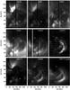 |
Fig. 1 EIS, AIA, and XRT images of the region analysed, i.e., six EIS spectral lines (Fe VIII, Fe IX, Fe XII, Fe XV, Fe XVI and Ca XVII, see Table 1), two AIA channels (171 Å, 94 Å), and one XRT channel (Ti_poly). The position of the hot (H) and cold (C) regions analysed here are marked in all images. |
In the same temporal window, we selected frames from two imagers, the X-ray telescope (XRT, Golub et al. 2007) on board Hinode (512′′ × 512′′ in Ti_poly filter, exposure times between 0.7 and 1 s) and the AIA on board SDO (full disk in 171 Å, 335 Å, 94 Å channels, exposure times 2, 2.9, 2.9 s, respectively).
The two sets of images were processed with the standard routines available in SolarSoft (xrt_prep and aia_prep). The images of the two instruments were co-aligned to each other (tr_get_disp.pro in SolarSoft) and to the EIS raster image in the He II 256 Å line, to match the EIS field of view. To improve the homogeneity between the XRT or AIA images and the EIS images, we have to consider that the latter are built from rastering that takes some time, while the former are “instantaneous”. We then built up new composite XRT and AIA images, which account for this different time spacing as follows: each vertical strip is extracted from the images closest in time to when the EIS slit was at that location. Figure 1 shows EIS, AIA, and XRT representative images of the same field of view and with the same timing. The EIS images are obtained by integrating the spectrum in a narrow band (0.1 Å wide) centered at the position of each line.
The information available for very hot plasma from EIS data is mostly based on the Ca XVII line, with the strongest EIS line formed around 6 MK (Del Zanna 2008). This line is severely blended with Fe XI and O V lines, as discussed in Young et al. (2007); Del Zanna (2009); Del Zanna et al. (2011a); Testa & Reale (2012). As in Paper I, in the case of the Ca XVII line we use the procedure developed by Ko et al. (2009) for de-blending the line from Fe XI and O V lines, and extract the Ca XVII emission.
The AIA and XRT images are composite images as explained above. The line images span emission from plasma in a broad temperature range 5.7 < log T < 6.7. The cold line images (log T < 6) show a very bright feature consisting of fan loops in the top-left region, consistent with the image in the AIA 171 Å channel. In the images around log T = 6.4 the morphology becomes very different: the whole region in the bottom part is quite bright and closed loops are visible, while where the bright cold features are present there is little emission. It has long been known that hot and cold emission is not often co-spatial, and this is often true even at high spatial resolution, such as that of AIA (Del Zanna 2013b). The Ca XVII image shows only two bright loops bifurcating southwards from a common point near the middle of the field of view. These features clearly show similar morphology to the AIA 94 Å emission, and are the same features found in Paper I. Here we also analyse XRT observations, which show that these loops are also bright in the X-rays. We see also some other emission around that recalls the EIS Fe XV and Fe XVI images.
Inside this field of view, we selected two small regions for more detailed analysis. In Paper I, a special three-colour coding is devised to highlight hot and cool regions immediately. In the three-colour image (where each colour is the intensity in a different AIA channel, green 171 Å, blue 335 Åand red 94 Å), we selected a strip 1-pixel wide and 7-pixels long, deep inside the hot region (where the hot part of the 94 Å emission is high), and another (equal) strip inside a colder region (high 171 Å emission, Fig. 2).
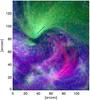 |
Fig. 2 Image of the active region in three AIA channels: 171 Å (green), 335 Å (blue), and 94 Å (red). We analyse in more detail the two small regions marked by the strips, one is hot (pink), the other is cold (green). |
We extracted EIS spectra in each pixel of the selected strips and, to increase the signal-to-noise ratio, we averaged the spectra over all the pixels in each strip. The resulting average spectra are shown in Figs. 3 and 4. In these spectra, the continuum is low and we see many emission lines for several elements, e.g., Fe, Ca, and Mg. We selected a subset of the emission lines with the following criterion. We conceptually divided the temperature range 5.5 < log T < 7 into bins Δlog T ~ 0.1 and chose approximately only one line that has the maximum formation temperature in a given bin, possibly the most intense one in at least one of the two spectra. We ended up with 14 lines, listed in Table 1, nine from Fe ions, three from Ca, and one from S and Mg, which provide a reasonably uniform coverage of the temperature range, as shown in Fig. 5. We use data from CHIANTI v 7.1 (Landi et al. 2013). We then fitted each line profile with a Gaussian (or multi-Gaussian for blended lines) and then we measured the flux by integrating the area below each Gaussian (Table 1). To each flux we applied the new EIS radiometric calibration, which also includes a correction for the long-term degradation of the EIS effective area (Del Zanna 2013a). This leads to significantly higher (by a factor of about two) radiances of the EIS lines in the long wavelength channel (245−290 Å). Our DEM modelling is mostly constrained by strong iron lines, for which the atomic data are reliable. To a first approximation, we can therefore neglect any uncertainty due to atomic data and chemical abundances. Since it is difficult to assess the accuracy of the new EIS calibration, we decided to associate only the uncertainty due to photon statistics with each flux, and then use the results of the DEM modelling to discuss systematic errors (see Sect. 3). We measure zero flux for the Ca XVII line in the cold region, and the value in the table is the corresponding upper limit.
2.1. The DEM reconstruction
We use the radiances in the selected lines (Table 1) to derive the distribution of the emission measure vs temperature, DEM(T). As a first step of the analysis, we use the EM loci method (Strong 1978), by which each line intensity is divided by its emissivity. The loci of these curves represent, at each temperature, the maximum value of the emission measure at that temperature, if the entire plasma were isothermal. Therefore, if the plasma were isothermal along the line of sight, all the curves would cross at a single point, exactly at the plasma temperature (see Del Zanna et al. 2002 for more details). There are many inversion methods to obtain the DEM.
We applied the widely-used Markov-chain Monte Carlo (MCMC, Kashyap & Drake 1998) method. This technique is based on a Bayesian statistical formalism to determine the most probable DEM curves that reproduce the observed line intensities by Monte Carlo simulations. A very useful feature of this technique is the possibility to obtain an estimate of the uncertainty of the DEM in each temperature bin in which the DEM is computed (see, e.g., Testa et al. 2011, 2012a for more detail).
For the application of the MCMC method, we assumed an electron density of 3 × 109cm-3, Feldman (1992) coronal abundances and CHIANTI 7.1 ionization equilibrium to compute the emissivity (per unit emission measure) of each line. The temperature range was divided into equal bins Δlog T ~ 0.1. Figure 6 shows the result of the reconstruction in which we added the EM-loci curves. We mark the most probable solution and the cloud of solutions in each temperature bin. The broader the cloud, the less constrained is the value of the best fit curve in that bin.
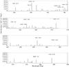 |
Fig. 3 Average Hinode/EIS spectrum over the strip in the cold region (green in Fig. 2). The lines selected for further analysis are marked and labelled (with their temperature of maximum formation, log T). |
There is no small region in the plot where EM-loci curves all intersect; the plasma is therefore clearly multi-thermal both in the cold and in the hot segments. The information about the very hot plasma comes mostly from the Ca lines. The very low flux of the Ca XVII line in the cold region puts a strong constraint that yields a very low emission measure for log T > 6.5, while the flux is much higher in the hot region. The Fe and Ca lines show a good overall agreement, while the Mg line leads to a higher emission measure in the cold region.
The MCMC method applied to the EIS data provides very different distributions in the cold and hot regions. In the cold region, the distribution is mostly flat for log T < 6.4, then it decreases rapidly. The local peak at log T = 6.3 might be significant, because of the small uncertainty. Overall the impression of a cool distribution is confirmed. In the hot region, we see a different trend: the DEM increases monotonically for log T > 6, with a slope between 2 and 3, it has a peak at log T = 6.6 and then decreases gradually at higher temperatures. This shape is not new for the active region core (Warren et al. 2011), but our treatment of uncertainties makes the solutions better constrained. In particular, the components on the hot side of the DEM peak look quite well defined even with respect to the cooler side, where several lines have maximum formation temperatures. These hot emission measure components are at a level of ~20% of the emission measure peak, and therefore a significant fraction.
Table 1 also contains the ratio of the line flux computed from the DEM reconstruction with the MCMC method to the observed line flux. Except for some well known lines (Mg VII, Fe XIII) and for hot lines (log T ≥ 6.45) in the cold region, not relevant for our analysis, good agreement (within 20%) is found, comparable to that obtained in other similar analyses (e.g., Warren et al. 2011).
In an attempt to better constrain the high temperature part of the DEM, first we add the
information provided by the flux measured in the 94 Å AIA channel. As we briefly discussed
previously, this band contains lines sensitive to emission from plasma at log T ~ 6.8 (Fe XVIII), but
also contains lines sensitive to lower temperatures, so the intensity in the AIA band can
be written as  (1)where EMcold and
EMhot are the emission
measures of the cold and hot components, and G94(Tcold)
and G94(Thot)
are the values of the channel response functions of the cold and hot peaks, respectively.
(1)where EMcold and
EMhot are the emission
measures of the cold and hot components, and G94(Tcold)
and G94(Thot)
are the values of the channel response functions of the cold and hot peaks, respectively.
We use the technique devised by Reale et al.
(2011) to separate the two contributions and pick up the hot one. The technique
uses the flux measured in the 171 Å channel: 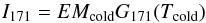 (2)to constrain the cold
component. Substituting in Eq. (1), we
obtain
(2)to constrain the cold
component. Substituting in Eq. (1), we
obtain  (3)We can then subtract the
flux extrapolated from the 171 Å channel from the 94 Å flux. What is left is the hot part
of the 94 Å emission:
(3)We can then subtract the
flux extrapolated from the 171 Å channel from the 94 Å flux. What is left is the hot part
of the 94 Å emission:  (4)that we show in Table
2, together with the corresponding ratio of the
flux from the DEM reconstruction (MCMC method) to the observed flux. We note that a
similar procedure, using the 171 and 193 Å AIA bands, was devised by Warren et al. (2012). Del Zanna
(2013b) suggested the use of the 171 and 211 Å AIA bands instead, the latter band
being used to estimate the contribution of the Fe XIV line to the 94 Å band. As shown in
Del Zanna (2013b), this method produces similar
results to the method of Warren et al. (2012). The
94 Å flux in the cold region is compatible with zero flux, so we imposed an upper limit as
we did for the Ca XVII flux in the same region in Table 1.
(4)that we show in Table
2, together with the corresponding ratio of the
flux from the DEM reconstruction (MCMC method) to the observed flux. We note that a
similar procedure, using the 171 and 193 Å AIA bands, was devised by Warren et al. (2012). Del Zanna
(2013b) suggested the use of the 171 and 211 Å AIA bands instead, the latter band
being used to estimate the contribution of the Fe XIV line to the 94 Å band. As shown in
Del Zanna (2013b), this method produces similar
results to the method of Warren et al. (2012). The
94 Å flux in the cold region is compatible with zero flux, so we imposed an upper limit as
we did for the Ca XVII flux in the same region in Table 1.
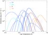 |
Fig. 5 Emissivity of the selected lines per unit emission measure. |
Fluxes measured in the AIA-94 Å channel and in the XRT-Ti_poly bands.
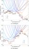 |
Fig. 6 Results of DEM reconstruction using the MCMC technique on 14 Hinode/EIS line fluxes (see text, and Table 1) for a) the cold region, b) the hot region, shown in Fig. 2. The red (histogram) curve is the solution that better reproduces the observed fluxes, the histogram cloud contains the solutions. The EM-loci curves are also shown for reference, each colour marks a different element. |
After including the information from the AIA 94 Å channel, the EM-loci AIA curves are in good agreement with the Ca XVII curves. In the hot region, the curves intersect both at log T ~ 6.6 and at log T ~ 6.8, but they are very similar in between. The DEM solutions derived with the MCMC method are very similar to those obtained without the AIA flux, thus confirming coherent information.
Additional information about the hot components is independently available from the X-ray observation with the Hinode/XRT. However, we expect looser constraints from the XRT filters because they are broadband, and have a broader temperature response. We can simply plug the flux measured in one XRT filter into our analysis; in particular, we consider the Ti_poly filter, which has the highest sensitivity to emission from plasma at log T ~ 6.9. The XRT flux and the related flux ratio are shown in Table 2. The XRT errors include the effect of the deterioration of the CCD response (Kobelski et al. 2013)1. The result, after including both AIA and XRT fluxes, is shown in Fig.7. The DEM in this figure is not qualitatively different from the DEM in Fig. 6, as expected from the broader AIA and XRT temperature responses (see EM-loci curve). A quantitative difference is that the DEM on the hot side of the DEM peak of the hot region is reduced by a factor ~2, i.e., to about 10% of the peak, while maintaining a narrow cloud distribution for log T < 6.9.
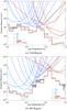 |
Fig. 7 Same as Fig. 6, adding the contribution of the fluxes measured in the “hot part" (see text) of the AIA 94 Å channel (black line) and in the XRT Ty_poly filter (red line). |
We further supported our analysis by comparing the best solutions of the DEM reconstruction on EIS data from the MCMC method with those from another method, devised by Del Zanna (1999). The method assumes that a smooth DEM distribution exists, and models it with a spline function. The choice of the nodes of the spline is somewhat subjective, but the actual inversion is carried out following the maximum entropy method described in Monsignori Fossi & Landini (1991). We note that the same atomic data and input parameters were used for both inversions. The comparison is shown in Fig. 8.
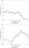 |
Fig. 8 Best DEM solutions from MCMC method (histogram, red in Fig. 6) and from the Del Zanna method (solid line + symbols) for a) the cold and b) the hot region. The emission measure values with MCMC are divided by the temperature to match the output from the Del Zanna method. |
The results from the spline method are obviously smoother, but overall there is very good agreement between the two methods for both regions, especially in the temperature ranges of interest, and in particular, in the hot part of the hot region. Good agreement (within 20%) between observed and predicted intensities is also found with this method.
3. Discussion and conclusions
We analysed the thermal distribution of the plasma along the line of sight in two different regions where the narrow-band imagers diagnosed two very different dominant temperatures (cool and hot). The analysis was mostly based on the spectral data from Hinode/EIS. Our major attention was to the hottest components that may be a signature of impulsive heating at work, and here our aim was to reconstruct the whole EM distribution and check the coherence of the overall scenario, including the hot component. At variance from many other similar analyses, our approach was to consider a limited number of spectral lines (~1 per temperature bin), and we picked the most intense lines uniformly covering the temperature range. In this way, we simplified our control and interpretation of the reconstruction results, and all measured fluxes had the same weight in determining the global emission measure distribution. We also had a particular approach regarding the assessment of the uncertainties. The typical choice is to associate the same percentage error with all measured fluxes; 20% is the most commonly assumed value (e.g., Warren et al. 2011). This uncertainty safely includes possible systematic unknown effects due to the instrument, atomic data, and chemical abundances, but weighs all measured values identically, independent of whether a line is strong or weak. Our choice is different. The measured fluxes were assigned the poissonian error exclusively, dictated only by the photon statistics. This allowed us to weigh the intense lines more heavily and to minimise the uncertainties of the solutions of the DEM reconstructions.
As a consequence, the DEM reconstruction with the MCMC technique leads to solution clouds with a narrow distribution around the best solution for many temperature bins (factor 2−3), which is significantly narrower than in previous works. Only a minority of temperature bins show a spread solution cloud. The constraint on the hot components is tighter.
The error estimate is important in this analysis, and we are aware that the real uncertainties are surely larger than those that we assume. The uncertainties can influence the error on the DEM solution considerably, and sometimes they can even influence the solution itself, as is thoroughly discussed in Testa et al. (2012b). We should also consider that the cloud spread may underestimate the real error on the DEM solution. The small uncertainties typically lead to a larger number of iterations with the MCMC method for better convergence (Testa et al. 2012b), but our 400 iterations are certainly an appropriate number for our cases. Tests show that DEM structures are reliably recovered on scales larger than Δlog T = 0.2, so we do not discuss narrower features.
The good agreement between predicted and observed line intensities confirms this, although we note that some significant discrepancies are present, in particular with the Ca XV line, as also found previously (Del Zanna 2013b). The good agreement between the two inversion methods, already found in Del Zanna et al. (2011b), is confirmed. This suggests that the main source of uncertainty resides in the choice of parameters, atomic data, and instrument calibration.
Although our assumptions probably underestimate the errors, the coherent support from other instruments (AIA, XRT), the agreement with the results from another reconstruction method, and the coherence with the morphology seen in the images spanning the different temperature regimes makes us confident that other errors should not affect our results considerably.
Overall, the analysis has confirmed the two general characteristics anticipated by the imagers. The comparison of the DEM distributions of the cold and hot regions has, on the one hand, revealed substantial thermal components for log T < 6.3 in the cold region, without showing prominent features. The reconstruction of the cold region also shows minor components for log T > 6.3. Since the images show no bright features in the hot channels and lines, we may use the values of these emission measure components as sensitivity limits of our analysis, i.e., we may not trust emission measure components below 1026 cm-5.
The hot region shows a much more peaked thermal structure, with the positive gradient typically found in previous studies in coronal loops of active region cores (Warren et al. 2011). The peak is at a rather high temperature (log T = 6.6) and beyond that the emission measure declines, but not very steeply, and still shows a significant fraction of emission measure at temperature log T ≤ 6.8. Some components might be present at even higher temperatures, although with higher uncertainties, up to the limit of the thermal sensitivity of our analysis (log T ~ 7). We believe that the joint use of hot spectral lines, AIA 94 Å channel and XRT filterbands, helps to partially remove the so-called blind spot for log T > 6.8 (Winebarger et al. 2012). Although the presence of the very hot component looks confirmed, still it is based on a very limited amount of information, and therefore some care should still be used. Some further feedback is provided by the comparison with the images and between the images. The morphology of the region in the Ca XVII line only partially overlaps the morphology in immediately cooler lines (Fe XVI), while it matches the X-ray and AIA 94 Å morphology well. This confirms that in the hot region selected in the present analysis there is indeed significant emission at 6 MK, resulting in strong Ca XVII. The Fe XVIII emission in the AIA 94 Å band is also due to this component, unlike other cases in the core of active regions where Ca XVII is not observed, and the Fe XVIII emission is due to a large emission measure at 3 MK (Del Zanna 2013b).
Our analysis has demonstrated how spectral data are by far more constraining than the data from imagers because the spectral lines are much more sensitive to temperature variations that the broader bands of the imagers (in agreement with the findings of Testa et al. 2012a). Still our analysis stresses that a quantum leap in the diagnostics of the hottest DEM components needs constraints from more lines sensitive to emission from high temperature plasma. These might be, for instance, easily accessible to broadband X-ray spectrometers, which we look forward to in future space missions.
Acknowledgments
A.P. and F.R. acknowledge support from Italian Ministero dell’Università e Ricerca (MIUR). G.D.Z. acknowledges support from STFC (UK). P.T. was supported by contract SP02H1701R from Lockheed-Martin, NASA contract NNM07AB07C to SAO, and NASA grant NNX11AC20G. CHIANTI is a collaborative project involving the NRL (USA), the Universities of Florence (Italy) and Cambridge (UK), and George Mason University (USA). Hinode is a Japanese mission developed and launched by ISAS/JAXA, with NAOJ, NASA, and STFC (UK) as partners, and operated by these agencies in cooperation with ESA and NSC (Norway). SDO data were supplied courtesy of the SDO/AIA consortium. SDO is the first mission to be launched for NASA’s Living With a Star Program. We thank the International Space Science Institute (ISSI) for hosting the International Team of S. Bradshaw and H. Mason: Coronal Heating – Using Observables to Settle the Question of Steady vs. Impulsive Heating.
References
- Culhane, J. L., Harra, L. K., James, A. M., et al. 2007, Sol. Phys., 243, 19 [Google Scholar]
- Del Zanna, G. 1999, Ph.D. Thesis, Univ. of Central Lancashire, UK [Google Scholar]
- Del Zanna, G. 2008, A&A, 481, L69 [NASA ADS] [CrossRef] [EDP Sciences] [Google Scholar]
- Del Zanna, G. 2009, A&A, 508, 501 [NASA ADS] [CrossRef] [EDP Sciences] [Google Scholar]
- Del Zanna, G. 2012, A&A, 546, A97 [NASA ADS] [CrossRef] [EDP Sciences] [Google Scholar]
- Del Zanna, G. 2013a, A&A, 555, A47 [NASA ADS] [CrossRef] [EDP Sciences] [Google Scholar]
- Del Zanna, G. 2013b, A&A, 558, A73 [NASA ADS] [CrossRef] [EDP Sciences] [Google Scholar]
- Del Zanna, G., Landini, M., & Mason, H. E. 2002, A&A, 385, 968 [NASA ADS] [CrossRef] [EDP Sciences] [Google Scholar]
- Del Zanna, G., Mitra-Kraev, U., Bradshaw, S. J., Mason, H. E., & Asai, A. 2011a, A&A, 526, A1 [NASA ADS] [CrossRef] [EDP Sciences] [Google Scholar]
- Del Zanna, G., O’Dwyer, B., & Mason, H. E. 2011b, A&A, 535, A46 [NASA ADS] [CrossRef] [EDP Sciences] [Google Scholar]
- Feldman, U. 1992, Phys. Scr., 46, 202 [CrossRef] [Google Scholar]
- Foster, A. R., & Testa, P. 2011, ApJ, 740, L52 [NASA ADS] [CrossRef] [Google Scholar]
- Golub, L., Deluca, E., Austin, G., et al. 2007, Sol. Phys., 243, 63 [NASA ADS] [CrossRef] [Google Scholar]
- Guarrasi, M., Reale, F., & Peres, G. 2010, ApJ, 719, 576 [NASA ADS] [CrossRef] [Google Scholar]
- Kashyap, V., & Drake, J. J. 1998, ApJ, 503, 450 [NASA ADS] [CrossRef] [Google Scholar]
- Klimchuk, J. A. 2006, Sol. Phys., 234, 41 [NASA ADS] [CrossRef] [Google Scholar]
- Ko, Y.-K., Doschek, G. A., Warren, H. P., & Young, P. R. 2009, ApJ, 697, 1956 [NASA ADS] [CrossRef] [Google Scholar]
- Kobelski, A. R., Saar, S. H., Weber, M. A., McKenzie, D. E., & Reeves, K. K. 2013, Sol. Phys., submitted [arXiv:1312.4850] [Google Scholar]
- Landi, E., Young, P. R., Dere, K. P., Del Zanna, G., & Mason, H. E. 2013, ApJ, 763, 86 [NASA ADS] [CrossRef] [Google Scholar]
- Lemen, J. R., Title, A. M., Akin, D. J., et al. 2012, Sol. Phys., 275, 17 [NASA ADS] [CrossRef] [Google Scholar]
- Martínez-Sykora, J., De Pontieu, B., Testa, P., & Hansteen, V. 2011, ApJ, 743, 23 [NASA ADS] [CrossRef] [Google Scholar]
- McTiernan, J. M. 2009, ApJ, 697, 94 [NASA ADS] [CrossRef] [Google Scholar]
- Monsignori Fossi, B. C., & Landini, M. 1991, Adv. Space Res., 11, 281 [Google Scholar]
- O’Dwyer, B., Del Zanna, G., Badnell, N. R., Mason, H. E., & Storey, P. J. 2012, A&A, 537, A22 [NASA ADS] [CrossRef] [EDP Sciences] [Google Scholar]
- Parker, E. N. 1988, ApJ, 330, 474 [Google Scholar]
- Patsourakos, S., & Klimchuk, J. A. 2009, ApJ, 696, 760 [NASA ADS] [CrossRef] [Google Scholar]
- Reale, F., McTiernan, J. M., & Testa, P. 2009a, ApJ, 704, L58 [NASA ADS] [CrossRef] [Google Scholar]
- Reale, F., Testa, P., Klimchuk, J. A., & Parenti, S. 2009b, ApJ, 698, 756 [CrossRef] [Google Scholar]
- Reale, F., Guarrasi, M., Testa, P., et al. 2011, ApJ, 736, L16 [NASA ADS] [CrossRef] [Google Scholar]
- Schmelz, J. T., Saar, S. H., DeLuca, E. E., et al. 2009, ApJ, 693, L131 [NASA ADS] [CrossRef] [Google Scholar]
- Shestov, S. V., Kuzin, S. V., Urnov, A. M., Ul’Yanov, A. S., & Bogachev, S. A. 2010, Astron. Lett., 36, 44 [NASA ADS] [CrossRef] [Google Scholar]
- Strong, K. T. 1978, Ph.D. Thesis, Univ. College London, UK [Google Scholar]
- Sylwester, B., Sylwester, J., & Phillips, K. J. H. 2010, A&A, 514, A82 [NASA ADS] [CrossRef] [EDP Sciences] [Google Scholar]
- Teriaca, L., Warren, H. P., & Curdt, W. 2012, ApJ, 754, L40 [NASA ADS] [CrossRef] [Google Scholar]
- Testa, P., & Reale, F. 2012, ApJ, 750, L10 [NASA ADS] [CrossRef] [Google Scholar]
- Testa, P., Reale, F., Landi, E., DeLuca, E. E., & Kashyap, V. 2011, ApJ, 728, 30 [NASA ADS] [CrossRef] [Google Scholar]
- Testa, P., De Pontieu, B., Martínez-Sykora, J., Hansteen, V., & Carlsson, M. 2012a, ApJ, 758, 54 [NASA ADS] [CrossRef] [Google Scholar]
- Testa, P., Drake, J. J., & Landi, E. 2012b, ApJ, 745, 111 [NASA ADS] [CrossRef] [Google Scholar]
- Testa, P., De Pontieu, B., Martínez-Sykora, J., et al. 2013, ApJ, 770, L1 [NASA ADS] [CrossRef] [Google Scholar]
- Warren, H. P., Brooks, D. H., & Winebarger, A. R. 2011, ApJ, 734, 90 [NASA ADS] [CrossRef] [Google Scholar]
- Warren, H. P., Winebarger, A. R., & Brooks, D. H. 2012, ApJ, 759, 141 [NASA ADS] [CrossRef] [Google Scholar]
- Winebarger, A. R., Warren, H. P., Schmelz, J. T., et al. 2012, ApJ, 746, L17 [NASA ADS] [CrossRef] [Google Scholar]
- Young, P. R., Del Zanna, G., Mason, H. E., et al. 2007, PASJ, 59, 857 [Google Scholar]
All Tables
All Figures
|
Fig. 1 EIS, AIA, and XRT images of the region analysed, i.e., six EIS spectral lines (Fe VIII, Fe IX, Fe XII, Fe XV, Fe XVI and Ca XVII, see Table 1), two AIA channels (171 Å, 94 Å), and one XRT channel (Ti_poly). The position of the hot (H) and cold (C) regions analysed here are marked in all images. |
| In the text | |
|
Fig. 2 Image of the active region in three AIA channels: 171 Å (green), 335 Å (blue), and 94 Å (red). We analyse in more detail the two small regions marked by the strips, one is hot (pink), the other is cold (green). |
| In the text | |
|
Fig. 3 Average Hinode/EIS spectrum over the strip in the cold region (green in Fig. 2). The lines selected for further analysis are marked and labelled (with their temperature of maximum formation, log T). |
| In the text | |
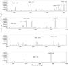 |
Fig. 4 As in Fig. 3 for the strip in the hot region (pink in Fig. 2). |
| In the text | |
|
Fig. 5 Emissivity of the selected lines per unit emission measure. |
| In the text | |
|
Fig. 6 Results of DEM reconstruction using the MCMC technique on 14 Hinode/EIS line fluxes (see text, and Table 1) for a) the cold region, b) the hot region, shown in Fig. 2. The red (histogram) curve is the solution that better reproduces the observed fluxes, the histogram cloud contains the solutions. The EM-loci curves are also shown for reference, each colour marks a different element. |
| In the text | |
|
Fig. 7 Same as Fig. 6, adding the contribution of the fluxes measured in the “hot part" (see text) of the AIA 94 Å channel (black line) and in the XRT Ty_poly filter (red line). |
| In the text | |
|
Fig. 8 Best DEM solutions from MCMC method (histogram, red in Fig. 6) and from the Del Zanna method (solid line + symbols) for a) the cold and b) the hot region. The emission measure values with MCMC are divided by the temperature to match the output from the Del Zanna method. |
| In the text | |
Current usage metrics show cumulative count of Article Views (full-text article views including HTML views, PDF and ePub downloads, according to the available data) and Abstracts Views on Vision4Press platform.
Data correspond to usage on the plateform after 2015. The current usage metrics is available 48-96 hours after online publication and is updated daily on week days.
Initial download of the metrics may take a while.