| Issue |
A&A
Volume 564, April 2014
|
|
|---|---|---|
| Article Number | A47 | |
| Number of page(s) | 9 | |
| Section | The Sun | |
| DOI | https://doi.org/10.1051/0004-6361/201322650 | |
| Published online | 03 April 2014 | |
The formation heights of coronal shocks from 2D density and Alfvén speed maps
Astrophysics Research Group, School of Physics, Trinity College Dublin, 2 Dublin, Ireland
Received: 11 September 2013
Accepted: 6 February 2014
Context. Super-Alfvénic shocks associated with coronal mass ejections (CMEs) can produce radio emission known as Type II bursts. In the absence of direct imaging, accurate estimates of coronal electron densities, magnetic field strengths, and Alfvén speeds are required to calculate the kinematics of shocks. To date, 1D radial models have been used, but these are not appropriate for shocks propagating in non-radial directions.
Aims. Here, we study a coronal shock wave associated with a CME and Type II radio burst using 2D electron density and Alfvén speed maps to determine the locations that shocks are excited as the CME expands through the corona.
Methods. Coronal density maps were obtained from emission measures derived from the Atmospheric Imaging Assembly (AIA) on board the Solar Dynamic Observatory (SDO) and polarized brightness measurements from the Large Angle and Spectrometric Coronagraph (LASCO) on board the Solar and Heliospheric Observatory (SOHO). Alfvén speed maps were calculated using these density maps and magnetic field extrapolations from the Helioseismic and Magnetic Imager (SDO/HMI). The computed density and Alfvén speed maps were then used to calculate the shock kinematics in non-radial directions.
Results. Using the kinematics of the Type II burst and associated shock, we find our observations to be consistent with the formation of a shock located at the CME flanks where the Alfvén speed has a local minimum.
Conclusions. The 1D density models are not appropriate for shocks that propagate non-radially along the flanks of a CME. Rather, the 2D density, magnetic field and Alfvén speed maps described here give a more accurate method for determining the fundamental properties of shocks and their relation to CMEs.
Key words: Sun: radio radiation / Sun: magnetic fields / Sun: corona / Sun: coronal mass ejections (CMEs)
© ESO, 2014
1. Introduction
Solar flares and coronal mass ejections (CMEs) are energetic manifestations of the restructuring coronal magnetic fields. As a CME travels through the corona, its velocity can become sufficiently larger than the background coronal Alfvén speed, causing a shock wave to form along its leading edge and/or flanks (Cho et al. 2007). It is within these shocks that electrons can be accelerated to near-relativistic energies to produce Type II radio signatures in low-frequency dynamic spectra (see Carley et al. 2013). Although CMEs and Type II radio bursts have been studied for many decades (see Pick et al. 2006), there remains unanswered questions in relation to where CME shocks are formed and how these phenomena are associated with the generation of Type II bursts.
It has long been suggested that Type II radio bursts are signatures of coronal shocks (Wild & McCready 1950; Uchida 1960). They appear as features slowly drifting toward lower frequencies at decimetric to kilometric wavelengths in dynamic radio spectra. This drift is the result of plasma emission generated by a super-Alfvénic shock traveling upwards in the corona (Cane et al. 1981), where density decreases with height. When direct low-frequency imaging is not available, a key problem is therefore the accurate calculation of the coronal density and Alfvén speed distributions with height. This is to relate the Type II emission frequency to its height and to investigate the direction of the shock propagation. The plasma frequency is related to the density of the emitting plasma by  , where C = 8980 Hz cm3/2 is a constant. To derive the shock kinematics, electron density models are normally employed to relate the plasma density to its coronal height and velocity. Specifically, the shock radial velocity is related to the plasma frequency drift rate, dfp/dt, and the electron density model, ne(r), by,
  (1)where v is the shock velocity, ne is the coronal plasma electron density and r is the heliocentric radial distance. Different coronal density models can therefore lead to differing kinematics. Several density models have been used to calculate the Type II shock position, such as the Newkirk (1961) model derived from the barometric height behavior of a gravitationally stratified corona, the Saito et al. (1977) model obtained from measurements of coronal polarized brightness (pB), and the Mann et al. (1999) model, derived from solutions of magnetohydrodynamic equations.
 |
Fig. 1 A variety of commonly used electron density models, which can give very different height estimates. For example, a density of 107 cm-3 can be located at ~1.4 R⊙ or ~2.0 R⊙, depending on the density model. Plotted for comparison, the set of density measurements obtained with Mars Express (MEX) between the years 2006−2008 (Verma et al. 2013). |
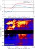 |
Fig. 2 GOES−15 soft X-ray light curve showing an X1.4 flare starting at 10:29:00 UT on 2011 Septemeber 22 (top) and the associated RSTO dynamic spectrum showing a Type II radio burst starting at 10:39:06 UT (bottom). This burst shows fundamental (F) and harmonic (H) emission. |
The use of an arbitrary radial density model can lead to an inaccurate calculation of shock heights and hence velocities. This is due to the significant difference in the shock height derived from different density models. An example is shown in Fig. 1, where an electron density of 107 cm-3, occurs at a height of 1.4 R⊙ for the Mann et al. (1999) model, while it occurs at a height of 2.0 R⊙ for the Allen-Baumbach model (Allen 1947). Another reason for an inaccurate shock height and velocity calculation is the time variability of the coronal density distribution (Parenti et al. 2000; Bemporad et al. 2003), which is not taken into account with typically employed density models. Finally, if a Type II radio source propagates non-radially, speeds derived from 1D radial density models underestimate the true shock speed.
Knowledge of the coronal density in the 2D plane is therefore crucial for determining accurate shock kinematics, while the knowledge of the 2D Alfvén speed is important to determine when the propagating shock reaches a super-Alfvénic speed. A 2D analytic model of the Alfvén speed was presented by Warmuth & Mann (2005). However, due to the temporal variability of the density and magnetic field in the corona, it is important to use observational data specific to the radio emission time rather than a generic analytic model for the Alfvén speed.
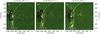 |
Fig. 3 SDO/AIA running-difference images of the erupting CME at 10:36:39−10:40:24 UT in the 211 Å passband. The CME leading edge is outside the field-of-view of SDO in panel a), while the propagation of the coronal bright front is visible at the location of the CME flanks at 10:38:38 UT panel b) and at 10:40:24 UT panel c). |
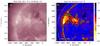 |
Fig. 4 SDO/AIA 211 Å passband intensity at 10:39:24 UT a) and the corresponding density map b). The contours show the harmonic plasma emission frequencies related to the measured coronal densities at 150, 200 and 300 MHz. The contours have been smoothed by a boxcar average of 3.6 arcsecs for display purposes, while dashed lines are at 1.0 R⊙ and 1.2 R⊙. |
Here, a new method to calculate coronal densities, magnetic field strengths, and Alfvén speeds in a 2D plane is presented. These 2D maps are then used to calculate the kinematics and the direction of propagation of a Type II radio burst observed on 2011 September 22. The Type II radio burst and coronal mass ejection (CME) are described in Sect. 2. The observational method and the models used to produce the 2D density maps are described in Sect. 3, while the Alfvén maps are shown in Sect. 4. Results are presented in Sect. 5, and finally, conclusions are discussed in Sect. 6.
2. Observations
On 2011 September 22, an X1.4 class flare was observed by GOES−15. The flare was identified to have originated in the NOAA active region 11302 and was associated with a CME eruption observed by the Atmospheric Imaging Assembly (AIA; Lemen et al. 2012) on board the Solar Dynamic Observatory (SDO; Pesnell et al. 2012) and by the Large Angle and Spectrometric Coronagraph (LASCO; Brueckner et al. 1995) on board the Solar and Heliospheric Observatory (SOHO; Domingo et al. 1995). The flare was followed by a Type II radio burst starting at 10:39:06 UT, which was observed with the e-Callisto spectrometer at the Rosse Solar-Terrestrial Observatory (RSTO; Zucca et al. 2012)1. In Fig. 2, the dynamic spectrum from RSTO (20−180 MHz) is shown together with its related GOES−15 soft X-ray light curve showing the X1.4 flare. The radio burst shows both fundamental (F) and harmonic (H) emission. The fundamental emission showing a drift rate of ~0.15 MHz s-1 is evident between 35 and 55 MHz, while the harmonic emission lies between 70 and 88 MHz reaching the FM broadcasting radio band.
The Type II related CME was observed at low altitude with the SDO/AIA 211 Å (Fe xiv) bandpass filter. Three running difference images are shown in Fig. 3, which are obtained by subtracting the image recorded one minute prior to the current time (i.e., five 211 Å frames previous). The CME leading edge is already outside the SDO field-of-view (FOV) at 10:36:39 UT (Fig. 3a), while the propagation of the coronal bright front related with the expansion of the CME flanks is visible at 10:38:38 UT (Fig. 3b) and at 10:40:24 UT (Fig. 3c).
In Fig. 4a, the intensity from SDO/AIA is shown at 10:39:24 UT. The corresponding coronal density map for this field of view (see Sect. 3.1), is shown in Fig. 4b. Higher in the corona, electron densities were obtained from pB images from LASCO C2. Only one polarization sequence is taken per day, so 02:57:00 UT was used in this work (see Sect. 3.2).
3. Density maps
Density was estimated using images from SDO/AIA for the height range 1−1.3 R⊙ and SOHO/LASCO for 2.5−5 R⊙. Unfortunately, there are no direct observations available at 1.3−2.5 R⊙. As a result, a data-constrained density model was used to interpolate between the SDO/AIA and SOHO/LASCO data coverage. In the following subsections the calculation of this map is described for the SDO/AIA density, the SOHO/LASCO density, and finally, the data-constrained analytic model.
3.1. SDO/AIA densities (<1.3 R⊙)
Electron densities were calculated from emission measure maps derived using the SDO/AIA’s six coronal filters and the method of Aschwanden et al. (2011). The method starts by reconstructing the differential emission measure dEM/dT (DEM) using the intensity of the six SDO/AIA filters for each pixel. The DEM is a measure of the amount of plasma along the line-of-sight (LOS) that contributes to the emitted radiation in the temperature range T to T + dT (Craig & Brown 1976). Once the column EM was obtained by integrating the DEM over the temperature range dT, the plasma electron density can be calculated by estimating an effective path length of the emitting plasma along the LOS. The 2D EM(r,φ) map, which is a function of heliocentric distance r and latitude φ, can then be written as, ![\begin{eqnarray} \label{Emission_measure} {\rm EM}(r,\phi) & =& \int{\left ( \frac{{\rm dEM}(r,\phi,T)}{{\rm d}T} \right ){\rm d}T}, \nonumber \\ & =& \int <N_\mathrm{e}^{2}(r,\phi)> {\rm d}s \mathrm{~~~~~~[cm^{-5}]}. \end{eqnarray}](/articles/aa/full_html/2014/04/aa22650-13/aa22650-13-eq23.png) (2)Knowing the effective LOS path length, s, the density of the emitting plasma can be obtained from the EM,
(2)Knowing the effective LOS path length, s, the density of the emitting plasma can be obtained from the EM, ![\begin{equation} N_\mathrm{e}(r,\phi)=\sqrt{\frac{{\rm EM}(r,\phi)}{s(r)}} \mathrm{~~~~~~[cm^{-3}]}. \end{equation}](/articles/aa/full_html/2014/04/aa22650-13/aa22650-13-eq25.png) (3)The effective LOS path length was calculated using a geometrical method used widely in stellar atmospheres (Menzel 1936) with a schematic of the problem shown in Fig. 5. The length of s changes at different heliocentric distances r, which contributes to the intensity of the emitting plasma measured by the observer. This gives the effective LOS path length using an asymptotic series expansion in the form,
(3)The effective LOS path length was calculated using a geometrical method used widely in stellar atmospheres (Menzel 1936) with a schematic of the problem shown in Fig. 5. The length of s changes at different heliocentric distances r, which contributes to the intensity of the emitting plasma measured by the observer. This gives the effective LOS path length using an asymptotic series expansion in the form,  (4)where H is the scale height. Using a typical coronal temperature of 2 MK, the scale height H measures ~9 × 109 cm and s ~ 4 × 1010 cm. The value of s does not significantly change in the 1−1.3 R⊙ range. The density map obtained with SDO/AIA centered on NOAA 11302, and the related harmonic plasma frequency contours at 150, 200, and 300 MHz are shown in Fig. 4b.
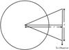 |
Fig. 5 Geometry for the emitting solar atmosphere effective LOS path length. The observer measures the contribution of the plasma emitting along the path s, which varies with the heliocentric distance r. |
3.2. SOHO/LASCO densities (>2.5 R⊙)
For the density calculation using SOHO/LASCO, we use pB images. The K-coronal brightness results from Thomson scattering of photospheric light by coronal electrons (Billings 1966). The intensity of scattered light and its polarization depends on the number of scattering electrons and a number of geometric factors, which was first outlined by Minnaert (1930). A method for estimating the electron density using these geometric factors and polarized brightness observations was first employed by van de Hulst (1947), which remains the standard procedure today. The F corona (arising from interplanetary dust scattering) must be eliminated from the data. In the case of pB observations at small elongations (≤5 R⊙; Mann 1992), the F corona can be assumed unpolarized and thus does not contribute to the pB signal; hence, we restrict our analysis to ≤5 R⊙. For full details on the calculation see Hayes et al. (2001).
3.3. Data-constrained density model (1.3−2.5 R⊙)
For the height range 1.3−2.5 R⊙, a combined plane-parallel and spherically-symmetric model, which is described below, was employed. Assuming a spherically-symmetric corona in hydrostatic equilibrium, the gradient of the pressure, P, is balanced by gravity, 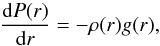 (5)where ρ(r) is the coronal plasma mass density and g(r) = GM⊙/r2. By integrating, using the ideal gas law (P = 2nkT), the spherically-symmetric (SS) density, nss(r), in an hydrostatic stratified corona is derived as,
 ![\begin{equation} \label{spherical_hydrostatic} n^{\mathrm{ss}}(r)=n^{\mathrm{ss}}_0\exp\left[-\frac{1}{H} \left(r-R_{\odot}\right) \right], \end{equation}](/articles/aa/full_html/2014/04/aa22650-13/aa22650-13-eq39.png) (6)where
(6)where  is the SS electron density at the solar surface (i.e., r = 1 R⊙), H(r) = kTr2/μmpGM⊙ is the scale height, k is the Boltzmann constant, T is the plasma temperature, μ is the mean molecular weight, mp is the proton mass, G is the gravitational constant and M⊙ is the solar mass. This expression holds well for quiet Sun conditions at large distances from the Sun (i.e., r > 2 R⊙).
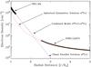 |
Fig. 6 Radial profile of the coronal density model constrained by densities from SDO/AIA and SOHO/LASCO. In blue, the plane-parallel solution reproduces the active region, (Eq. (7)), and in red, the spherical-symmetric solution reproduces the quiet Sun (Eq. (6)). The combined model in orange (Eq. (8)) is used to replace the missing data in the range 1.3−2.5 R⊙. |
Low in the solar atmosphere, where r ≪ 2 R⊙, this reduces to the plane-parallel (PP) solution, ![\begin{equation} \label{planeparallel_hydrostatic} n^{\mathrm{pp}}(r)=n^{\mathrm{pp}}_0\exp\left[-\frac{1}{H_0}(r-R_{\odot}) \right], \end{equation}](/articles/aa/full_html/2014/04/aa22650-13/aa22650-13-eq50.png) (7)where
(7)where  is the PP electron density, H0 = kT/μmpg⊙ is the scale height, and g⊙ is the acceleration due to gravity, which are all defined at the solar surface (i.e., r = 1R⊙).The PP solution is a good approximation of the electron density distribution in the low corona and in active regions (see, Aschwanden et al. 2001).
In this work, we simultaneously model the outer corona using the SS model (r > 2 R⊙) and the possible presence of a PP active region at r < 2 R⊙ using,  (8)This was then used to interpolate the observational data between 1.3 R⊙ and 2.5 R⊙. Figure 6 presents an example electron density radial profile with data from SDO/AIA and SOHO/LASCO. The PP solution (Eq. (7)) is displayed in blue. It reproduces the density enhancement of an active region well, but it decays too fast to reproduce the quiet Sun (QS) density at large coronal heights. The SS solution (Eq. (6)) is displayed in red and it reproduces the quiet Sun coronal density. The combined PP and SS model (Eq. (8)) is displayed in orange. The combined model fits the observational data well and is employed in producing the density map for the height range 1.3−2.5 R⊙, which is shown in Fig. 7. The map shows the difference in electron density between polar and equatorial regions and the presence of coronal streamers and active regions are clear. Electron density at different position angles for the heights of 1.1 and 1.3 R⊙ are shown in Fig. 8. Coronal holes (CH) have a density of ~3 × 10⁷ electrons cm-3 at 1.1 R⊙ at the position angle of ~170° and ~1 × 107 cm-3 at 1.3 R⊙. Meanwhile, active regions (AR) reach a density of ~2 × 108 cm-3 at 1.1 R⊙ at a position angle of ~70° and ~9 × 107 cm-3 at 1.3 R⊙. These density maps are in good agreement with those derived using EUV line ratios by Gallagher et al. (1999).
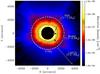 |
Fig. 7 2D electron density map on 2011 September 22 obtained from SDO/AIA (1−1.3 R⊙) and SOHO/LASCO (2.5−5 R⊙) with an interpolated electron density from the density model given in Eq. (8) (1.3−2.5 R⊙). |
 |
Fig. 8 Electron density at different position angles (PA) for heights of 1.1 R⊙ and 1.3 R⊙. Coronal holes measure a density of ~3 × 107 cm-3 at 1.1 R⊙ and ~1 × 107 cm-3 at 1.3 R⊙, while the active regions reach a density of ~2 × 108 cm-3 at 1.1 R⊙ and ~9 × 107 cm-3 at 1.3 R⊙. |
4. Alfvén speed maps
The Alfvén speed, which is the speed at which information travels in a magnetized plasma, was obtained by combining measurements of electron density (described in Sect. 3) and magnetic field strength. Specifically, the 2D Alfvén speed map was calculated using a 2D magnetic field plane obtained from 3D magnetic extrapolations, which are described in the following section.
4.1. Magnetic field
The coronal magnetic field strength was obtained from the potential-field source-surface (PFSS) extrapolation, which is based on Schatten et al. (1969) and the software of Schrijver & De Rosa (2003)2. The PFSS package combines measured LOS photospheric magnetograms with an evolving surface flux transport model. This provides full solar surface coverage by evolving magnetic flux that rotates over the Earth-viewed western limb to cover the far side of the Sun. This spherical surface is then used as the lower boundary condition for the PFSS extrapolation, which provides a vector magnetic field solution for a 3D grid of polar coordinates (r− radial distance; θ− longitude; φ− latitude). The vector field is described by components in the direction of each of the polar coordinates (i.e., Br, Bθ, Bφ), such that the total magnetic field, B, is given by 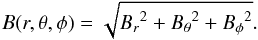 (9)One limitation to this model is the handling of magnetic field that emerges on the far side of the Sun. Such fields may not be fully present in the PFSS model for several days after their location rotates over the Earth-viewed eastern limb. This is due to the gradual transition from only flux-transported fields at and behind the eastern limb to only measured fields some distance onto the visible disk.
At the time of the event studied here (2011 September 22 10:39 UT), the photospheric signature of NOAA 11302 was not present in the PFSS model due to its proximity to the east limb (heliographic coordinates N11E81). This region first appears in the PFSS lower boundary on 2011 September 24 but shows significant flux imbalance until 2011 September 26. The PFSS model used here was taken from 2011 September 26 at 12:04 UT, and the effective Earth-viewed plane-of-sky (POS) from 2011 September 22 was extracted. This was achieved by averaging B(r,θ,φ) over a ±10° range of longitudes, θ, centered on both the AR Carrington longitude and its 180°-separated location; the result is shown in Fig. 9b.
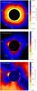 |
Fig. 9 a) 2D electron density map from 2011 September 22. b) The magnetic field strength obtained with PFSS extrapolation, and c) the Alfvén speed map obtained from the electron density and magnetic field strength values (Eq. (10)). The active region (AR), quiet Sun (QS), and coronal hole (CH) radial profiles used in Fig. 10 are also shown. |
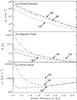 |
Fig. 10 a) Electron density at a function of height for an active region (PA = 75°) the quiet Sun (PA = 270°) and coronal hole (PA = 165°). b) Magnetic field strength is shown for the same position angles. c) Calculated Alfvén speed for the three profiles. Active region (AR), coronal hole (CH), and quiet Sun (QS) profiles are displayed in Fig. 9. |
 |
Fig. 11 Distance-time plot at different propagation angles of the CME observed with SDO/AIA running difference images (red data points) and of the Type II radio burst using different non-radial density profiles (green data points). The SDO distance-time plot was obtained by plotting the intensity of the running difference image (grey scale) for the specific trace over time. The Type II distance-time was obtained by plotting the dynamic spectra with the frequency axis converted in height using the density of the correspondent non-radial trace for the harmonic emission. The considered profiles on top of the active region is shown on the inset of each plot. The profiles are marked with white traces separated by 10°; the profile used is marked with a red trace. a) The distance-time plot for the northern flank region at +40° from the radial trace; and b) distance-time for the Radial profile (0°), while the distance-time for the southern flank region at −60° from the radial trace is in panel c). |
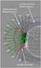 |
Fig. 12 Running difference image of the CME observed with SDO/AIA 211 Å passband at 10:40:24 UT with superimposed, non-radial profiles used to calculate the Type II radio burst and CME kinematics (black traces). Traces showing matching kinematics between the CME and the Type II burst are marked in green. The red contours are the Nançay NRH emission at 150 MHz at 10:40:26 UT. The blue contours are the harmonic plasma emission at 70 and 150 MHz estimated from the density map. The suggested locations of the Type II burst at the CME flanks are positioned at the intersection between the CME front (indicated with the dashed black curve) and the 70 MHz harmonic plasma frequency contour (in blue). |
4.2. Alfvén speed
The 2D map of Alfvén speed, vA(r,φ), is obtained using the electron density and the magnetic field maps by  (10)Figures 9a and 9b present the 2D maps of density and magnetic field used to calculate the Alfvén speed. At the base of the corona, the extrapolated magnetic field reaches ~500 G in active regions, while it reaches ~3−10 G outside of active regions (i.e., across both quiet Sun and coronal hole regions). The resulting 2D Alfvén speed map is shown in Fig. 9c. The Alfvén speed reaches ~104 km s-1 in active regions and decreases to ~200 km s-1 in local minima in neighboring QS regions. Also notable are the relatively high Alfvén speeds (~1000 km s-1) in coronal holes because the magnetic field in CHs decreases more slowly than that in ARs and the electron density is significantly lower in CHs than in ARs. Radial profiles of density, magnetic field, and Alfvén speed are shown in Figs. 10a−c, respectively, for an active region (PA = 75°), quiet Sun (PA = 270°) and coronal hole regions (PA = 165°).
5. Results and discussion
A CME was observed low in the corona with SDO/AIA (Fig. 3), which is the candidate for triggering the Type II radio burst observed with RSTO (Fig. 2). To verify this, the kinematics of the Type II burst and the CME were calculated. The kinematics of the Type II radio burst were calculated relating the plasma frequency measured in the dynamic spectrum to its electron density ( ). The position of the shock is then obtained by relating the emitting electron plasma density to its position on the calculated density map (Fig. 7). To date, this has been done by employing radial models of the coronal density even if Type II radio bursts propagate often non-radially.
Using the calculated 2D density map, non-radial density traces from NOAA 11302 were extracted. The traces, which start at the solar region from the solar limb, have 10 degree separation from the radial trace (α = 0°) with positive values toward solar north and negative values toward solar south. For each of the non-radial profiles a distance-time plot for the CME and the Type II radio burst was obtained. The CME kinematics were obtained using SDO/AIA 211 Å running difference images. Three example frames of running difference images are shown in Fig. 3. For each of the non-radial traces, a distance-time plot was obtained. In Fig. 11, three example distance-time plots are shown for α = + 40°, 0°, −60°. The CME distance-time evolution obtained from the running difference intensity along the non-radial trace is displayed in gray scale with explicit data points in red. The Type II radio burst dynamic spectra are displayed in red-blue color scale, where frequency has been converted into distance along the non-radial trace. This was achieved using the density obtained along that trace and by considering a harmonic plasma emission. The data points related with the position of the harmonic emission are displayed in green. The panel at the left of each plot indicates the considered non-radial trace. Comparable kinematics were found between the SDO/AIA front and the Type II radio burst position for α between −60° and + 40° (green traces in Fig. 12). We note that the SDO FOV limits the maximum observable height to ~1.3 R⊙ for near-radial traces (e.g., α between −20° and + 20°), making the kinematic comparison with the Type II radio burst complicated. In addition, the SDO running difference front for these traces (see Fig. 11a) is most likely related with the loop structure emerging below the CME leading edge, which is already outside the FOV of SDO (see Fig. 3).
 |
Fig. 13 Propagation speed calculated for the CME and the Type II radio burst for two different non-radial profiles in the “flank” region at α = + 40° and α = −60° (profiles are displayed on the insets). The calculated Alfvén speed is displayed in the shaded region. |
In Fig. 12, the SDO/AIA 211 Å running difference image shows the lower portion of the CME at 10:40:24 UT with the Nançay radio heliograph (NRH; Kerdraon & Delouis 1997) emission at 150 MHz, which is superimposed as red contours (40%, 60%, 70%, and 90% of the peak flux). The NRH emission at 150 MHz shows a brightness temperature of log 10T = 7.1, while the dynamic spectrum at 150 MHz shows a faint continuum (Fig. 2). This emission is most likely originated from the CME plasma (see, Ramesh 2005). The relation of the 150 MHz emission and the CME is also evident from the spatial correspondence of the NRH contours and the CME flanks. The harmonic plasma emission contours at 70 and 150 MHz were calculated from the density map are displayed in blue. The 70 MHz contour corresponds to the frequency of the Type II shock upstream region (harmonic emission in Fig. 2). The 150 MHz contour is shown for height comparison with the NRH emission. We suggest two locations where the Type II radio burst could be originated; these positions at the CME flanks are located where the 70 MHz contour (Type II upstream region) intersects the CME front edge (indicated with a black dashed line) at a height of ~1.6 R⊙. For the same CME eruption, Carley et al. (2013) found that a series of herringbone radio bursts have originated along the southern flank as it expands through the corona. This agrees with our finding of comparable kinematics between the Type II shock and the CME expansion in the southern flank region (i.e., α = −60°).
The speeds of the CME and of the Type II radio burst for the flank regions (α = + 40°, −60°) are compared with the Alfvén speed (shaded area) in Fig. 13. The Alfvén speed was extracted along the non-radial traces (α = + 40°, −60°) from the 2D map shown in Fig. 9c. The CME flank speed remains sub-Alfvénic, while the Type II burst shows a super-Alfvénic speed. The Type II burst in the flank regions reaches a max speed of ~1400 km s-1 and then decelerates to ~700 km s-1. This deceleration may result in the fading of the Type II burst in the dynamic spectra as the burst speed approaches the local Alfvén speed.
6. Conclusion
A new method to obtain semi-empirical 2D maps of coronal density and Alfvén speed has been presented. Using these calculated maps, a decametric Type II burst and a CME that occurs on 2011 September 22, were analyzed to understand their relationship.
The analysis of the Type II kinematics, using the 2D density maps, have been performed for non-radial profiles in the POS starting from the active region. Previously, analytical radial density models have been employed to calculate the radio burst kinematics (e.g., Robinson 1985; Vršnak et al. 2002). Using a 2D density map at the specific time of the radio burst and performing a non-radial analysis, we were able to relate the Type II burst with the CME and discriminate which portion of the CME front was responsible for triggering the Type II emission. Comparing the CME kinematics calculated for different non-radial traces to the Type II burst we find evidence for the shock to be formed in the flank region of the CME. This agrees with previous interpretations (e.g., Claßen & Aurass 2002; Mancuso & Raymond 2004). By calculating the height of the upstream shock front (70 MHz) using the 2D density map and relating it to the position of the CME, we were able to locate the position of the shock in the CME flanks at a height of ~1.6 R⊙.
In addition, we were able to compare the Type II burst shock speed with the local Alfvén speed using the 2D Alfvén speed maps. The Type II burst speed was found to be super-Alfvénic (e.g., Vršnak & Cliver 2008; Cho et al. 2005; Klein et al. 1999). Furthermore, the decelerating phase of the Type II shock can be related with the fading of the Type II burst in the dynamic spectrum as the shock approaches the local Alfvén speed.
The method used to construct 2D density and Alfvén speed maps presented in this work can be used for the study of all Type II radio bursts. These time specific semi-empirical maps improve the calculation of shock kinematics and represent a step forward from the standardized radial density profiles currently employed. Further investigation relating the kinematics of the limb event of Type IIs and CMEs using the 2D maps and radio imaging is necessary. This can be done with Type II radio bursts in the NRH frequency range (i.e., 150−445 MHz) where direct radio imaging can be used to locate the position of the burst, or with lower frequency imaging telescopes, such as the LOw Frequency ARray (LOFAR; van Haarlem et al. 2013).
Acknowledgments
P.Z. is supported by a TCD Innovation Bursary. EC is a Government of Ireland Scholar supported by the Irish Research Council. D.S.B. is supported by the European Space Agency Prodex programme. We are grateful to the SDO, LASCO and Nançay NRH team for the open access data. We are grateful to David Long for the beneficial discussions and help.
References
- Allen, C. W. 1947, MNRAS, 107, 426 [NASA ADS] [Google Scholar]
- Aschwanden, M. J., Schrijver, C. J., & Alexander, D. 2001, ApJ, 550, 1036 [NASA ADS] [CrossRef] [Google Scholar]
- Aschwanden, M. J., Boerner, P., Schrijver, C. J., & Malanushenko, A. 2011, Sol. Phys., 384 [Google Scholar]
- Bemporad, A., Poletto, G., & Romoli, M. 2003, Mem. Soc. Astron. It., 74, 721 [NASA ADS] [Google Scholar]
- Bougeret, J. L., Goetz, K., Kaiser, M. L., et al. 2008, Space Sci. Rev., 136, 487 [NASA ADS] [CrossRef] [Google Scholar]
- Billings, D. E. 1966, A guide to the Solar Carona (New York: Academic Press) [Google Scholar]
- Brueckner, G. E., Howard, R. A., Koomen, M. J., et al. 1995, Sol. Phys., 162, 357 [NASA ADS] [CrossRef] [Google Scholar]
- Cane, H. V., Stone, R. G., Fainberg, J., et al. 1981, Geophys. Res. Lett., 8, 1285 [Google Scholar]
- Carley, E. P., McAteer, R. T. J., & Gallagher, P. T. 2012, ApJ, 752, 36 [NASA ADS] [CrossRef] [Google Scholar]
- Carley, E. P., Long, D. M., Byrne, J. P., et al. 2013, Nature Phys., 2767 [Google Scholar]
- Claßen, H. T., & Aurass, H. 2002, A&A, 384, 1098 [NASA ADS] [CrossRef] [EDP Sciences] [Google Scholar]
- Cho, K.-S., Moon, Y.-J., Dryer, M., et al. 2005, J. Geophys. Res., 110, 12101 [NASA ADS] [CrossRef] [Google Scholar]
- Cho, K.-S., Lee, J., Moon, Y.-J., et al. 2007, A&A, 461, 1121 [NASA ADS] [CrossRef] [EDP Sciences] [Google Scholar]
- Craig, I. J. D., & Brown, J. C. 1976, A&A, 49, 239 [NASA ADS] [Google Scholar]
- Domingo, V., Fleck, B., & Poland, A. I. 1995, Sol. Phys., 162, 1 [NASA ADS] [CrossRef] [Google Scholar]
- Elmore, D. F., Burkepile, J. T., Darnell, J. A., Lecinski, A. R., & Stanger, A. L. 2003, Proc. SPIE, 4843, 66 [NASA ADS] [CrossRef] [Google Scholar]
- Gallagher, P. T., Mathioudakis, M., Keenan, F. P., Phillips, K. J. H., & Tsinganos, K. 1999, ApJ, 524, L133 [NASA ADS] [CrossRef] [Google Scholar]
- Hannah, I. G., & Kontar, E. P. 2012, A&A, 539, A146 [NASA ADS] [CrossRef] [EDP Sciences] [Google Scholar]
- Hanser, F. A., & Sellers, F. B. 1996, Proc. SPIE, 2812, 344 [Google Scholar]
- Hayes, A. P., Vourlidas, A., & Howard, R. A. 2001, ApJ, 548, 1081 [NASA ADS] [CrossRef] [Google Scholar]
- Kerdraon, A., & Delouis, J.-M. 1997, Coronal Physics from Radio and Space Observations, Proc. of the CESRA Workshop, 483, 192 [Google Scholar]
- Klein, K.-L., Khan, J. I., Vilmer, N., Delouis, J.-M., & Aurass, H. 1999, A&A, 346, L53 [NASA ADS] [Google Scholar]
- Lemen, J. R., Title, A. M., Akin, D. J., et al. 2012, Sol. Phys., 275, 17 [NASA ADS] [CrossRef] [Google Scholar]
- Mancuso, S., & Raymond, J. C. 2004, A&A, 413, 363 [NASA ADS] [CrossRef] [EDP Sciences] [Google Scholar]
- Mann, I. 1992, A&A, 261, 329 [NASA ADS] [Google Scholar]
- Mann, G., Jansen, F., MacDowall, R. J., Kaiser, M. L., & Stone, R. G. 1999, A&A, 348, 614 [NASA ADS] [Google Scholar]
- Mann, G., Klassen, A., Aurass, H., & Classen, H.-T. 2003, A&A, 400, 329 [NASA ADS] [CrossRef] [EDP Sciences] [Google Scholar]
- Menzel, D. H. 1936, Harvard College Observatory Circular, 417, 1 [NASA ADS] [Google Scholar]
- Minnaert, M. 1930, Z. Astrophys., 1, 209 [NASA ADS] [Google Scholar]
- Newkirk, G., Jr. 1961, ApJ, 133, 983 [NASA ADS] [CrossRef] [Google Scholar]
- Parenti, S., Bromage, B. J. I., Poletto, G., et al. 2000, A&A, 363, 800 [NASA ADS] [Google Scholar]
- Pesnell, W. D., Thompson, B. J., & Chamberlin, P. C. 2012, Sol. Phys., 275, 3 [NASA ADS] [CrossRef] [Google Scholar]
- Pick, M., Forbes, T. G., Mann, G., et al. 2006, Space Sci. Rev., 123, 341 [NASA ADS] [CrossRef] [Google Scholar]
- Quémerais, E., & Lamy, P. 2002, A&A, 393, 295 [NASA ADS] [CrossRef] [EDP Sciences] [Google Scholar]
- Ramesh, R. 2005, Coronal and Stellar Mass Ejections, IAU Symp. Proc., 226, 83 [NASA ADS] [Google Scholar]
- Roberts, J. A. 1959, Aust. J. Phys., 12, 327 [NASA ADS] [CrossRef] [Google Scholar]
- Robinson, R. D. 1985, Sol. Phys., 95, 343 [NASA ADS] [CrossRef] [Google Scholar]
- Saito, K., Poland, A. I., & Munro, R. H. 1977, Sol. Phys., 55, 121 [NASA ADS] [CrossRef] [Google Scholar]
- Schatten, K. H., Wilcox, J. M., & Ness, N. F. 1969, Sol. Phys., 6, 442 [Google Scholar]
- Schrijver, C. J., & De Rosa, M. L. 2003, Sol. Phys., 212, 165 [Google Scholar]
- Uchida, Y. 1960, PASJ, 12, 376 [NASA ADS] [Google Scholar]
- van de Hulst, H. C. 1947, ApJ, 105, 471 [NASA ADS] [CrossRef] [Google Scholar]
- van Haarlem, M. P., Wise, M. W., Gunst, A. W., et al. 2013, A&A, 556, A2 [NASA ADS] [CrossRef] [EDP Sciences] [Google Scholar]
- Verma, A. K., Fienga, A., Laskar, J., et al. 2013, A&A, 550, A124 [Google Scholar]
- Vourlidas, A., Buzasi, D., Howard, R. A., & Esfandiari, E. 2002, Solar Variability: From Core to Outer Frontiers, ESA Publ. Division, 506, 91 [Google Scholar]
- Vršnak, B., & Cliver, E. W. 2008, Sol. Phys., 253, 215 [NASA ADS] [CrossRef] [Google Scholar]
- Vršnak, B., Magdalenić, J., Aurass, H., & Mann, G. 2002, A&A, 396, 673 [NASA ADS] [CrossRef] [EDP Sciences] [Google Scholar]
- Warmuth, A., & Mann, G. 2005, A&A, 435, 1123 [NASA ADS] [CrossRef] [EDP Sciences] [Google Scholar]
- Wild, J. P., & McCready, L. L. 1950, Austral. J. Sci. Res. A Physical Sciences, 3, 387 [NASA ADS] [Google Scholar]
- Zucca, P., Carley, E. P., McCauley, J., et al. 2012, Sol. Phys., 94 [Google Scholar]
All Figures
|
Fig. 1 A variety of commonly used electron density models, which can give very different height estimates. For example, a density of 107 cm-3 can be located at ~1.4 R⊙ or ~2.0 R⊙, depending on the density model. Plotted for comparison, the set of density measurements obtained with Mars Express (MEX) between the years 2006−2008 (Verma et al. 2013). |
| In the text | |
|
Fig. 2 GOES−15 soft X-ray light curve showing an X1.4 flare starting at 10:29:00 UT on 2011 Septemeber 22 (top) and the associated RSTO dynamic spectrum showing a Type II radio burst starting at 10:39:06 UT (bottom). This burst shows fundamental (F) and harmonic (H) emission. |
| In the text | |
|
Fig. 3 SDO/AIA running-difference images of the erupting CME at 10:36:39−10:40:24 UT in the 211 Å passband. The CME leading edge is outside the field-of-view of SDO in panel a), while the propagation of the coronal bright front is visible at the location of the CME flanks at 10:38:38 UT panel b) and at 10:40:24 UT panel c). |
| In the text | |
|
Fig. 4 SDO/AIA 211 Å passband intensity at 10:39:24 UT a) and the corresponding density map b). The contours show the harmonic plasma emission frequencies related to the measured coronal densities at 150, 200 and 300 MHz. The contours have been smoothed by a boxcar average of 3.6 arcsecs for display purposes, while dashed lines are at 1.0 R⊙ and 1.2 R⊙. |
| In the text | |
|
Fig. 5 Geometry for the emitting solar atmosphere effective LOS path length. The observer measures the contribution of the plasma emitting along the path s, which varies with the heliocentric distance r. |
| In the text | |
|
Fig. 6 Radial profile of the coronal density model constrained by densities from SDO/AIA and SOHO/LASCO. In blue, the plane-parallel solution reproduces the active region, (Eq. (7)), and in red, the spherical-symmetric solution reproduces the quiet Sun (Eq. (6)). The combined model in orange (Eq. (8)) is used to replace the missing data in the range 1.3−2.5 R⊙. |
| In the text | |
|
Fig. 7 2D electron density map on 2011 September 22 obtained from SDO/AIA (1−1.3 R⊙) and SOHO/LASCO (2.5−5 R⊙) with an interpolated electron density from the density model given in Eq. (8) (1.3−2.5 R⊙). |
| In the text | |
|
Fig. 8 Electron density at different position angles (PA) for heights of 1.1 R⊙ and 1.3 R⊙. Coronal holes measure a density of ~3 × 107 cm-3 at 1.1 R⊙ and ~1 × 107 cm-3 at 1.3 R⊙, while the active regions reach a density of ~2 × 108 cm-3 at 1.1 R⊙ and ~9 × 107 cm-3 at 1.3 R⊙. |
| In the text | |
|
Fig. 9 a) 2D electron density map from 2011 September 22. b) The magnetic field strength obtained with PFSS extrapolation, and c) the Alfvén speed map obtained from the electron density and magnetic field strength values (Eq. (10)). The active region (AR), quiet Sun (QS), and coronal hole (CH) radial profiles used in Fig. 10 are also shown. |
| In the text | |
|
Fig. 10 a) Electron density at a function of height for an active region (PA = 75°) the quiet Sun (PA = 270°) and coronal hole (PA = 165°). b) Magnetic field strength is shown for the same position angles. c) Calculated Alfvén speed for the three profiles. Active region (AR), coronal hole (CH), and quiet Sun (QS) profiles are displayed in Fig. 9. |
| In the text | |
|
Fig. 11 Distance-time plot at different propagation angles of the CME observed with SDO/AIA running difference images (red data points) and of the Type II radio burst using different non-radial density profiles (green data points). The SDO distance-time plot was obtained by plotting the intensity of the running difference image (grey scale) for the specific trace over time. The Type II distance-time was obtained by plotting the dynamic spectra with the frequency axis converted in height using the density of the correspondent non-radial trace for the harmonic emission. The considered profiles on top of the active region is shown on the inset of each plot. The profiles are marked with white traces separated by 10°; the profile used is marked with a red trace. a) The distance-time plot for the northern flank region at +40° from the radial trace; and b) distance-time for the Radial profile (0°), while the distance-time for the southern flank region at −60° from the radial trace is in panel c). |
| In the text | |
|
Fig. 12 Running difference image of the CME observed with SDO/AIA 211 Å passband at 10:40:24 UT with superimposed, non-radial profiles used to calculate the Type II radio burst and CME kinematics (black traces). Traces showing matching kinematics between the CME and the Type II burst are marked in green. The red contours are the Nançay NRH emission at 150 MHz at 10:40:26 UT. The blue contours are the harmonic plasma emission at 70 and 150 MHz estimated from the density map. The suggested locations of the Type II burst at the CME flanks are positioned at the intersection between the CME front (indicated with the dashed black curve) and the 70 MHz harmonic plasma frequency contour (in blue). |
| In the text | |
|
Fig. 13 Propagation speed calculated for the CME and the Type II radio burst for two different non-radial profiles in the “flank” region at α = + 40° and α = −60° (profiles are displayed on the insets). The calculated Alfvén speed is displayed in the shaded region. |
| In the text | |
Current usage metrics show cumulative count of Article Views (full-text article views including HTML views, PDF and ePub downloads, according to the available data) and Abstracts Views on Vision4Press platform.
Data correspond to usage on the plateform after 2015. The current usage metrics is available 48-96 hours after online publication and is updated daily on week days.
Initial download of the metrics may take a while.