| Issue |
A&A
Volume 564, April 2014
|
|
|---|---|---|
| Article Number | A97 | |
| Number of page(s) | 16 | |
| Section | The Sun | |
| DOI | https://doi.org/10.1051/0004-6361/201322147 | |
| Published online | 11 April 2014 | |
Rayleigh-Taylor instability in partially ionized compressible plasmas: One fluid approach
1 Instituto de Astrofísica de Canarias, 38205, C/vía Láctea, s/n, 38205 La Laguna, Tenerife, Spain
2 Departamento de Astrofísica, Universidad de La Laguna, 38205 La Laguna, Tenerife, Spain
e-mail: This email address is being protected from spambots. You need JavaScript enabled to view it.
; This email address is being protected from spambots. You need JavaScript enabled to view it.
; This email address is being protected from spambots. You need JavaScript enabled to view it.
Received: 26 June 2013
Accepted: 20 December 2013
Abstract
Aims. We study the modification of the classical criterion for the linear onset and growth rate of the Rayleigh-Taylor instability (RTI) in a partially ionized (PI) plasma in the one-fluid description by considering a generalized induction equation.
Methods. The governing linear equations and appropriate boundary conditions, including gravitational terms, are derived and applied to the case of the RTI in a single interface between two partially ionized plasmas. The boundary conditions lead to an equation for the frequencies in which some have positive complex parts, marking the appearance of the RTI. We study the ambipolar term alone first, extending the result to the full induction equation later.
Results. The configuration is always unstable because of the presence of a neutral species. In the classical stability regime, the growth rate is small, since the collisions prevent the neutral fluid to fully develop the RTI. For parameters in the classical instability regime, the growth rate is lowered, but the differences with the compressible MHD case are small for the considered theoretical values of the collision frequencies and diffusion coefficients for solar prominences.
Conclusions. The PI modifies some aspects of the linear RTI instability, since it takes into account that neutrals do not feel the stabilizing effect of the magnetic field. For the set of parameters representative for solar prominences, our model gives the resulting timescale comparable to observed lifetimes of RTI plumes.
Key words: instabilities / Sun: oscillations / Sun: corona / Sun: filaments, prominences
© ESO, 2014
1. Introduction
One of the well-known fluid instabilities that has been applied widely in many different astrophysical contexts is the Rayleigh-Taylor instability (RTI), which appears when a lighter fluid supports or accelerates a heavier one. We can cite as examples: the RTI in planetary nebulas (Bucciantini et al. 2004), supernova explosions (Fryxell et al. 1991), acretion disks (Wang & Nepveu 1983), relativistic jets (Matsumoto & Masada 2013), the evolution of the inner layers of red giants (Eggleton et al. 2006), the formation of hydrogen clouds in the local bubble (Breitschwerdt et al. 2000), the solar atmospheric flux tubes (Parker 1979), and prominences (Isobe et al. 2005). These topics are among the vast literature regarding this instability in astrophysical plasmas.
The starting point of these studies is the classical hydrodynamic instability with the addition of a magnetic field. To study the Rayleigh-Taylor instability in magnetohydrodynamics (MHD), it is better to use the divergence-free velocity condition (which is the type of movement more likely to produce instabilities, since the energy is not wasted in compressing the plasma). Hence, the dispersion relation for the two fluids with densities ρ1 and ρ2 that lay one below the other with a magnetic field parallel to the contact surface is (Chandrasekhar 1961; Priest 1982), 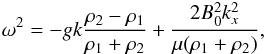 (1)where B0 is the magnetic field strength, k is the modulus of the wavenumber, kx is the component of the wavenumber along the magnetic field direction, ky the component across the field, g is the acceleration of gravity, and μ is the magnetic permittivity. The hydromagnetic case is recovered if no magnetic field is considered, which means that the configuration is unstable if ρ2>ρ1. The magnetic field stabilizes perturbations down to a critical value of kx along its direction, but the field cannot stabilize perturbations across the field (kx = 0) no matter how strong it might be.
Other effects, such as compressibility, viscosity, tension forces, relativistic corrections, magnetic fields perpendicular to the surface or other types of stratification, and forces may introduce corrections to the classical stability criterion and linear growth rate of the RTI. Compressibility is normally the leading effect, which must be taken into account in most of the applications. There have been many studies of the effect of compressibility in the magnetic RTI (see for example Vandervoort 1961; Shivamoggi 1982; Bernstein & Book 1983; Ribeyre et al. 2004; Livescu 2004; Shivamoggi 2008; Liberatore & Bouquet 2008, and references therein). These studies show that the compressibility has mainly a stabilizing influence by lowering the linear growth rates, although the stability threshold that appears in Eq. (1) is not modified. On the other hand, by considering only this extra effect greatly complicates the solution, so simple relations, such as Eq. (1), are no longer obtained.
Prominences are a very likely candidate to display the RTI in the solar atmosphere, since they are composed of cool and dense plasma surrounded by much lighter coronal plasma (see the reviews Labrosse et al. 2010; Mackay et al. 2010). The magnetic field plays a key role in the structure and dynamics of prominences; hence, the RTI must be studied in the context of the MHD theory. Using computational techniques allow us to directly solve the MHD partial differential equations and study the non-linear regime of the RTI. These numerical studies of RTI (see for example Jun et al. 1995; Arber et al. 2007; Stone & Gardiner 2007) agree with the results of the linear theory and show some new interesting features, such as the growth enhancement of bubbles and fingers in the non-linear regime across the field, since it prevents secondary Kelvin-Helmholtz instabilities and mixing between the fluids. This non-linear phase agrees qualitatively with the observations of turbulent plumes and bubbles in prominences (Isobe et al. 2005; Berger et al. 2008, 2010, 2011; Heinzel et al. 2008; Ryutova et al. 2010) and has even been used to infer plasma properties from observational features (Hillier et al. 2012b). The presence of the RTI has also been confirmed numerically in more general prominence models with 3D geometry (Isobe et al. 2006; Hillier et al. 2011, 2012a,c).
Prominences also have another feature that can be relevant for the RTI because of their physical properties, namely partial ionization. Since prominences are relatively cool and dense objects, their plasma is expected to be partially ionized (Patsourakos & Vial 2002; Gilbert et al. 2007; Labrosse et al. 2010; Zaqarashvili et al. 2011b). The ionization degree of the prominence plasma has not been directly measured with accuracy but the plasma is neither in a completely ionized state or is a neutral gas with the typical physical parameters of this objects. This partially ionized prominence plasma can no longer be described with a one-fluid ideal MHD. Chhajlani & Vaghela (1989) studied the magnetic RTI in a two-fluid model without considering the full dynamics of the neutral fluid (which was only subject to collisions) and concluded that the stability threshold is not changed, but the growth rate is lowered. A two-fluid description with one neutral and one ion-electron fluid coupled only by ion-neutral collision (without electron collisions and diffusive terms in the induction equation) was considered in Soler et al. (2012b) for the Kelvin-Helmholtz instability due to shear flow at an interface between two partially ionized plasmas and for the RTI in a similar setup in Díaz et al. (2012). The conclusion in Díaz et al. (2012) was that the instability threshold of the RTI is modified, so the configuration with heavier fluid on the top of lighter fluid is always unstable. However, the linear growth rate is substantially reduced depending on the parameters. This approach has also been used by Shadmehri et al. (2013) in the context of the RTI in the borders of the local bubble, where partial ionization also plays a relevant role.
Our main objective in this paper is to study the stability threshold and the linear growth rate of the RTI in a plasma described in a one-fluid model. This takes into account the partial ionization effects in the form of a generalized induction equation and considers all the types of collisions, forces present, and the diffusive terms in the induction equation. We develop a general formulation, having in mind its global applicability to different astrophysical situations. After this general formulation has been set, we particularize it to the case of solar prominences and consider the importance of the different terms in the induction equation (many of them neglected in previous works) for the development of the RTI in this environment. We compare our results with those from the simple two-fluid approach in Díaz et al. (2012) and try to understand the linear phase of the RTI in a partially ionized plasma to use it as a comparison with more complicated computational models with complex geometry and the non-linear stages.
2. Multi-fluid equations for partially ionized plasma
2.1. Fluid equations for each species
The general transport equations for a multi-component plasma can be derived from the Boltzmann kinetic equation, taking into acount general properties of the collisions terms (Braginskii 1965; Bittencourt 1986; Balescu 1988). The most common form of the MHD theory can only be applied to totally ionized plasma, where the different species are completely coupled dynamically and thermally by collisions, so partial ionization cannot be described. The first extension from MHD in the presence of neutrals for strong collisional coupling is to only consider the modifications due to collisions in the generalized Ohm’s law and energy transport (Braginskii 1965; Khodachenko et al. 2004; Forteza et al. 2007), by assuming a strong thermal coupling and neglecting the transport coefficients. Another way of including partial ionization effects is to use a multi-fluid treatment, where ions and electrons are considered together as an ion-electron fluid (due to their strong electromagnetic coupling) and neutrals are separately considered with as many neutral species as one wishes to include (see, e.g., Zaqarashvili et al. 2011b,a; Soler et al. 2012a). The two-fluid approach (a hydrogen plasma only considered) was used in Díaz et al. (2012) for studying the RTI with the additional neglection of other diffusive terms in the induction equation. Here, we take the single fluid approach by combining the equations for each species in a single fluid equation and obtaining a generalized form of the MHD equations valid for PI plasmas.
We proceed with the derivation of the generalized one-fluid equations starting from the macroscopic equations for each species. In the following expressions, the subscripts i, n, and e stand for ions, neutrals, and electrons, respectively. The momentum equation for each species is ![Mathematical equation: \begin{eqnarray} \rho_{\rm e} \left( \frac{\partial {\vec v}_{\rm e}}{\partial t} + {\vec v}_{\rm e} \cdot \nabla {\vec v}_{\rm e} \right) &=& -\nabla p_{\rm e} - e n_{\rm e} \left( {\vec E} + {\vec v}_{\rm e} \times {\vec B} \right) + \rho_{\rm e} {\vec g} + {\vec R}_{\rm e}, \nonumber \\[-1.5mm] \rho_{\rm i} \left( \frac{\partial {\vec v}_{\rm i}}{\partial t} + {\vec v}_{\rm i} \cdot \nabla {\vec v}_{\rm i} \right) &=& -\nabla p_{\rm i} + e n_ {\rm i}\left( {\vec E} + {\vec v}_{\rm i} \times {\vec B} \right) + \rho_{\rm i} {\vec g} + {\vec R}_{\rm i}, \nonumber \\[-1.5mm] \rho_{\rm n} \left( \frac{\partial {\vec v}_{\rm n}}{\partial t} + {\vec v}_{\rm n} \cdot \nabla {\vec v}_{\rm n} \right) &=& -\nabla p_{\rm n} + \rho_{\rm n} {\vec g} + {\vec R}_{\rm n}, \label{3fluid_eqs} \end{eqnarray}](/articles/aa/full_html/2014/04/aa22147-13/aa22147-13-eq12.png) (2)where vi, ve, and vn are the velocity of the ion, electron, and neutral fluid, respectively; pi, pe, and pn are the pressure of the ion, electron and the neutral fluid, respectively; ρi, ρe and ρn are the ion, electron and neutron densities, respectively; and Ri, Re, and Rn are the momentum transfer terms due to collisions for ions, electrons, and neutrals, respectively. We also define the total density ρ = ρn + ρi, the neutral fraction ξn = ρn/ρ, and the ion fraction ξi = ρi/ρ, with ξn + ξi = 1. Hence, the parameter ξn indicates the ionization degree from ξn = 0 for a fully ionized plasma to ξn = 1 for a neutral gas. We have assumed the non-diagonal terms of the pressure tensors to be negligible and the diagonal terms to be equal, so the pressure tensor becomes isotropic and can be represented by the scalar pressure. The elastic collision term of each species is approximated as (Braginskii 1965; Bittencourt 1986)
(2)where vi, ve, and vn are the velocity of the ion, electron, and neutral fluid, respectively; pi, pe, and pn are the pressure of the ion, electron and the neutral fluid, respectively; ρi, ρe and ρn are the ion, electron and neutron densities, respectively; and Ri, Re, and Rn are the momentum transfer terms due to collisions for ions, electrons, and neutrals, respectively. We also define the total density ρ = ρn + ρi, the neutral fraction ξn = ρn/ρ, and the ion fraction ξi = ρi/ρ, with ξn + ξi = 1. Hence, the parameter ξn indicates the ionization degree from ξn = 0 for a fully ionized plasma to ξn = 1 for a neutral gas. We have assumed the non-diagonal terms of the pressure tensors to be negligible and the diagonal terms to be equal, so the pressure tensor becomes isotropic and can be represented by the scalar pressure. The elastic collision term of each species is approximated as (Braginskii 1965; Bittencourt 1986) 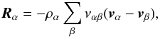 (3)where ναβ is the collisional frequency of species α with particles of species β. For our three species, they become
 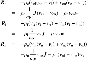 (4)with w = vi − vn as the diffusion velocity of ions with respect to neutrals and J = ene(vi − ve) as the total current density. This form of the friction momentum transfer does not alter the one-fluid equations of mass conservation and momentum conservation from their MHD counterparts when written in terms of the overall velocity of the plasma, v = ∑ α = i,e,i(ραvα) /ρ ≈ ξivi + ξnvn. However, the energy equation has to take into account the currents arising from these non-MHD terms, and an additional equation for the evolution of the magnetic field, namely a generalized induction equation, is also required to close the system.
2.2. Equation for the diffusion velocity
To obtain the momentum equation for the diffusion velocity w, we proceed as follows. The momentum equation for electrons and ions are added up, neglecting the electron inertial terms because of the small electron mass compared to the other species. We do not neglect the electron gravity compared to the ion gravity yet (ρeg compared to ρig), 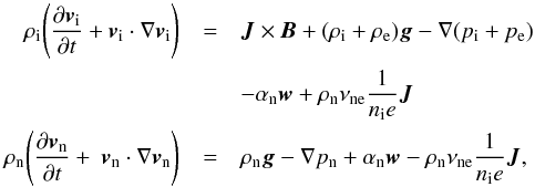 (5)with the definition for the coefficient of friction between the plasma and the neutral gas as
  (6)Now, we add the upper equation multiplied by ξn and lower equation, multiplied by − ξi. The result is:
 ![Mathematical equation: \begin{eqnarray} \xi_{\rm i} \xi_{\rm n} \rho \left( \frac{{\rm D}_{\rm i} {\vec v}_{\rm i}}{{\rm D}t} -\frac{{\rm D}_{\rm n} {\vec v}_{\rm n}}{{\rm D}t} \right ) = \xi_{\rm n} \left[{\vec J} \times {\vec B} \right] - {\vec G} - \alpha_{\rm n} {\vec w} \nonumber \\ + \rho_{\rm n} \nu_{\rm ne} \frac{1}{n_{\rm i} e} {\vec J} + \xi_{\rm n} \rho_{\rm e} {\vec g}, \label{dif_eq1} \end{eqnarray}](/articles/aa/full_html/2014/04/aa22147-13/aa22147-13-eq46.png) (7)where
(7)where 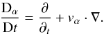 (8)We have taken into account that ξi + ξn = 1, thus the gravity terms for ions and neutrals cancel out and the electron term might become relevant. This gravitional term is similar to those of the electron inertia that have been already neglected, but we keep it here to check its magnitude, especially since the RTI is driven by gravity. It is therefore important to assure its effect as much as possible. Regarding the pressure gradients, we have introduced the new PI pressure terms following Braginskii (1965) as
  (9)We still have the ion and neutral inertia terms in Eq. (7). These are neglected on the basis of the following argument. We can express the total derivative in terms of the diffusion velocity
 ![Mathematical equation: \begin{eqnarray} \left(\frac{{\rm D}_{\rm i} {\vec v}_{\rm i}}{{\rm D}t} - \frac{{\rm D}_{\rm n} {\vec v}_{\rm n}}{{\rm D}t} \right) &=& \frac{\partial {\vec w}}{\partial t} + (\xi_{\rm n}-\xi_{\rm i}) {\vec w} \cdot \nabla {\vec w} \nonumber \\[2mm] &&+\,{\vec w} \cdot \nabla {\vec v} + {\vec v} \cdot \nabla {\vec w} \approx \frac{\partial {\vec w}}{\partial t}\cdot \end{eqnarray}](/articles/aa/full_html/2014/04/aa22147-13/aa22147-13-eq50.png) (10)In a linear regime, all the advection terms in this equation are second order effects, and the remaining time derivative of w can be neglected when compared with the friction terms, which are of the order of w/τcol with τcol ~ 1/ναβ being the characteristic timescale related to collisions.
(10)In a linear regime, all the advection terms in this equation are second order effects, and the remaining time derivative of w can be neglected when compared with the friction terms, which are of the order of w/τcol with τcol ~ 1/ναβ being the characteristic timescale related to collisions.
Taking all the aforementioned simplifications into account, we obtain an expression for the diffusion velocity between ions and neutrals: 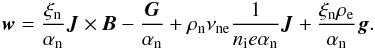 (11)From this expression, we can see that the ion and neutral fluids do not follow each other exactly, which raises additional dissipative effects. On the other hand, by neglecting the inertial terms, we have obtained an explicit expression for the diffusion velocity in terms of other variables, assuming that collisions lead to the terminal values of w given by Eq. (11). These are much faster than the evolution of the remaining variables. Thus, the velocities of the ion and neutral species do not longer appear in the equations and the diffusion velocity w can be computed from the single-fluid variables.
2.3. Induction equation
To proceed further, we need a generalized Ohm’s law and an induction equation to obtain an equation for the magnetic field evolution. These are obtained from the momentum equation for electrons in Eq. (2), again neglecting their inertial terms. After some algebra we obtain ![Mathematical equation: \begin{eqnarray} {\vec E} + {\vec v}\times{\vec B} &=& -\xi_{\rm n} \, {\vec w}\times{\vec B} + \frac{1}{n_{\rm i} e} {\vec J}\times{\vec B} \nonumber \\[2mm] &&- \frac{\nabla p_{\rm e}}{e n_{\rm e}} + \alpha_{\rm e} \frac{1}{n_{\rm i}^2{\rm e}^2} {\vec J} - \frac{\rho_{\rm e}\nu_{\rm en}{\vec w}}{en_{\rm e}} + \frac{\rho_{\rm e}}{n_{\rm e} e} {\vec g}, \label{ohmlaw} \end{eqnarray}](/articles/aa/full_html/2014/04/aa22147-13/aa22147-13-eq55.png) (12)with the definition αe = ρe(νei + νen). We then substitute the expression for the diffusion velocity in Eq. (11) and insert the result in Faraday’s law, obtaining
(12)with the definition αe = ρe(νei + νen). We then substitute the expression for the diffusion velocity in Eq. (11) and insert the result in Faraday’s law, obtaining ![Mathematical equation: \begin{eqnarray} \frac{\partial{\vec B}}{\partial t} &=& {\vec \nabla}\times \left[ ({\vec v}\times{\vec B}) - \frac{{\vec J}}{\sigma} -\left( \frac{1-2\varepsilon\xi_{\rm n}}{en_{\rm e}}{\vec J}\times{\vec B}\right) \right. \nonumber \\[2mm] &&+ \left. \left( \frac{\xi_{\rm n}^2}{\alpha_{\rm n}}({\vec J}\times{\vec B}) \times{\vec B}\right) - \left( \frac{\varepsilon{\vec G} - \nabla p_{\rm e}}{en_{\rm e}} \right)- \left(\frac{\xi_{\rm n}}{\alpha_{\rm n}}{\vec G}\times{\vec B} \right) \right. \nonumber \\[2mm] && \left. -\,\left( \frac{\rho_{\rm e}}{e n_{\rm e}} (1+\xi_{\rm n} \varepsilon) {\vec g} + \frac{\xi_{\rm n}^2 \rho_{\rm e}}{\alpha_{\rm n}} {\vec g} \times {\vec B} \right) \right] \label{eq_induction} \end{eqnarray}](/articles/aa/full_html/2014/04/aa22147-13/aa22147-13-eq57.png) (13)with the definitions of ε = ρeνen/αn (which is a small parameter) and the Ohmic conductivity σ = (ene)2/(αe − ε2αn). In this equation, the terms on the right hand side are: ideal MHD induction term, Ohmic term, Hall term, ambipolar term, generalized battery term (which includes a part already present in fully ionized plasmas and a part depending on partial ionization by means of G), a G × B term of perpendicular currents caused by these pressure gradients (similar to the Hall term with currents), and gravity terms (again with a similar g × B part also included). We can define the coefficients in the different terms as
(13)with the definitions of ε = ρeνen/αn (which is a small parameter) and the Ohmic conductivity σ = (ene)2/(αe − ε2αn). In this equation, the terms on the right hand side are: ideal MHD induction term, Ohmic term, Hall term, ambipolar term, generalized battery term (which includes a part already present in fully ionized plasmas and a part depending on partial ionization by means of G), a G × B term of perpendicular currents caused by these pressure gradients (similar to the Hall term with currents), and gravity terms (again with a similar g × B part also included). We can define the coefficients in the different terms as 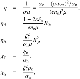 (14)with η, ηH, ηA, χp, and χg being the ohmic diffusivity, Hall diffusivity, ambipolar diffusivity, and coefficients related to the battery and gravity terms, respectively. Assuming that the acceleration of gravity is uniform, the curl of the second to last term in Eq. (13) vanishes, and the induction equation is finally written as
 ![Mathematical equation: \begin{eqnarray} \frac{\partial{\vec B}}{\partial t} &=& {\vec \nabla}\times \left[ \rule{0mm}{3.5mm} ({\vec v}\times{\vec B}) - \eta \nabla \times {\vec B} - \eta_\mathrm{H} \left(\nabla \times {\vec B} \right) \times{\vec B}/B_0 \right. \nonumber \\ &&+ \left. \rule{0mm}{3.5mm} \eta_\mathrm{A} \left\{ \left( \nabla \times {\vec B} \right) \times{\vec B} \right\} \times{\vec B} /B_0^2 - \left(\varepsilon{\vec G} - \nabla p_{\rm e} \right) /(en_{\rm e}) \right. \nonumber \\ &&- \left. \rule{0mm}{3.5mm}\chi_\mathrm{p} {\vec G}\times{\vec B} - \chi_\mathrm{g} {\vec g} \times {\vec B} \right], \label{ind_etas} \end{eqnarray}](/articles/aa/full_html/2014/04/aa22147-13/aa22147-13-eq70.png) (15)in which we used Ampere’s law (neglecting Maxwell’s displacement current) to eliminate the current density in terms of the magnetic field, J = ∇ × B/μ. Equation (15) is a very general form of the induction equation in the one-fluid description of partial ionized plasmas, and it is a generalization of the well-known generalized induction equation in classical textbooks (see for example Braginskii 1965) with all the pressure gradient, gravity terms, and the expressions of the diffusion coefficients.
(15)in which we used Ampere’s law (neglecting Maxwell’s displacement current) to eliminate the current density in terms of the magnetic field, J = ∇ × B/μ. Equation (15) is a very general form of the induction equation in the one-fluid description of partial ionized plasmas, and it is a generalization of the well-known generalized induction equation in classical textbooks (see for example Braginskii 1965) with all the pressure gradient, gravity terms, and the expressions of the diffusion coefficients.
The formulation of the induction equation in Eq. (15) allows for very general analyses that can be useful in a broad context of astrophysical plasmas. Some of the terms are a priory expected to be smaller than others (as those related to the electron mass), but others cannot be ruled out just from general considerations. We discuss their importance for a case with parameter values appropriate for solar prominences below. We describe next the plasma and magnetic field configuration used to study the RTI in this environment in Sect. 3 and then explore the effect of the leading term under these conditions in Sect. 4, namely, with the ambipolar diffusion 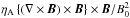 . Then, we consider the full induction equation in Sect. 5 to test the magnitude of the remaining terms and finish discussing the results and drawing our conclusions.
3. Reference configuration
Since we aim to obtain some extensions to the well-known formula in Eq. (1), we restrict the analysis to the simple configuration of a contact surface following the classical analysis in Chandrasekhar (1961), Drazin & Reid (1981), Priest (1982), which is amenable to analytical solutions. We use this configuration to study the RTI in prominence threads, especially for choosing the values of the equilibrium and perturbation parameters, but the method developed in this paper is general and can be applied to other astrophysical situations, which involve the RTI in PI plasmas.
The reference configuration consists of two regions filled with uniform plasmas composed of ions, electrons, and neutrals separated by a contact surface at z = 0. We use Cartesian coordinates and denote the quantities in the plasma below the discontinuity (z< 0) with a subscript 1 and those in the plasma above the discontinuity (z> 0) with a subscript 2. The magnetic field permeating the plasma is uniform and tangent to the discontinuity, so  . Since gravity is perpendicular to it, the gravity direction is g = −gẑ. The whole configuration is invariant in the x and y-directions.
 |
Fig. 1 Sketch of the equilibrium configuration used in the analysis of this work. The equilibrium state is a contact surface between two regions filled uniformly with plasma having different properties with the lower quantities labelled as “1” and the upper ones as “2”. The magnetic field is uniform and directed along the x-axis, while the whole configuration is invariant in the x- and y-directions. |
In absence of hydrostatic pressure gradients or flows, the plasma described in the previous paragraph is not in equilibrium, since nothing counteracts the gravity force. We are not interested in the overall equilibrium, only in the local region where the instability is triggered. More precisely, the equilibrium pressure gradient ∇p0 is related to the gravitational scale height, while the perturbed quantities vary on a much shorter spatial scale. Hence, we assume that all the plasma magnitudes (namely the density, the pressure, and the ionization degree) are constant in each zone. Pressure balance along the discontinuity demands that the total pressure for each species must be equal in each side, and since the magnetic field is assumed to be uniform, this means the gas pressures are equal in each side (p1 = p2). On the other hand, the temperature, density, and ionization degree on each region are parameters of our model. Since we are interested in studying the RTI, we assume that ρ2>ρ1. No ionization-recombination processes are included, so the ionization degree in each region remains constant. Note also that the plasma beta  is then constant all over the domain.
Another important simplification in this particular configuration is that we can neglect the variations in the coefficients in Eq. (14) during the evolution of the instability. The equilibrium field satisfies ∇ × B0 = 0, so there are no currents in the reference state and the only contribution of the diffusive terms to the first-order induction equation are those with the coefficients calculated in the reference configuration.
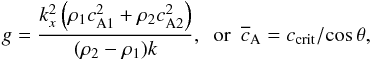
Finally, using this reference configuration, the classical instability criterion (Eq. (1)) can be written in the following form  (16)with θ being the angle between the equilibrium magnetic field and the wavevector k and k the wavevector modulus (wavenumber). We define the critical speed as
 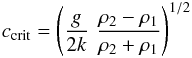 (17)and the reduced square Alfvén speed as
  (18)with the usual definition for the squared Alfvén speed
  , so
, so 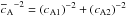 . It is convenient then to use
  as a parameter. Notice that we have
  in the case of a prominence with ρ2 ≫ ρ1, so this averaged Alfvén speed is approximately the Alfvén speed in the prominence.
4. MHD and ambipolar diffusion
It is clear that dealing with the all the terms in Eq. (15) is very difficult. Hence, we first concentrate in the modifications introduced in the ideal MHD theory by the ambipolar term, which has proved to be relevant in solar atmospheric situations (see for example Khodachenko et al. 2004; Arber et al. 2007; Khomenko & Collados 2012, and references therein). We neglect all the magnetic diffusion terms in this section except the ambipolar one, obtaining a simple form of the induction equation, 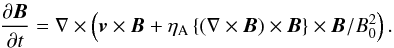 (19)The mass and momentum conservation equations are not modified by the presence of ambipolar diffusion. In addition, we assume an adiabatic energy equation plus the contribution from the ambipolar diffusion term (neglecting transport terms such as conduction, radiation of other heating sources). Hence, after deriving the energy term corresponding to the ambipolar diffusion, our system of basic equations is
 ![Mathematical equation: \begin{eqnarray} &&\frac{\partial \rho}{\partial t} = - \nabla \cdot \left( \rho {\vec v} \right), \nonumber \\ &&\rho \frac{\partial {\vec v}}{\partial t} = - \rho {\vec v} \cdot \nabla {\vec v} -\nabla p + \frac{1}{\mu} \left( \nabla \times {\vec B}\right) \times {\vec B} + \rho {\vec g}, \nonumber \\ &&\frac{\partial {\vec B}}{\partial t} = \nabla \times \left( {\vec v} \times {\vec B} + \eta_\mathrm{A} \left\{ \left( \nabla \times {\vec B} \right) \times{\vec B} \right\} \times{\vec B} /B_0^2 \right),\nonumber \\ &&\frac{\partial p}{\partial t} = - {\vec v} \cdot \nabla p - \gamma p \nabla \cdot {\vec v} \nonumber \\ &&\qquad\; + (\gamma-1) \frac{\eta_\mathrm{A}}{\mu B_0^2} \left(\nabla \times {\vec B} \right) \times \left[ \left\{ \left( \nabla \times {\vec B} \right) \times{\vec B} \right\} \times{\vec B} \right], \end{eqnarray}](/articles/aa/full_html/2014/04/aa22147-13/aa22147-13-eq96.png) (20)where γ is the adiabatic index and p = pi + pe + pn the total scalar pressure of the fluid.
(20)where γ is the adiabatic index and p = pi + pe + pn the total scalar pressure of the fluid.
4.1. Linearized equations
Next, we study linear perturbations from the uniform state. To obtain a general formulation, we label the reference quantities with the subscript 0 and the linear perturbations without subscript (B = B0x + b). The subscript 0 can be replaced with 1 of 2 when one of the regions in which the physical domain is considered, but otherwise, the deduction is valid for any uniform configuration.
Since no equilibrium flow is present (v0 = 0), all the advection terms are second order effects. No currents are present in the reference state, so the term in the energy equation coming from the ambipolar diffusion is also a second order effect and can be neglected in the linealized problem. Hence, we are left with a considerably simpler system of differential equations, namely
 (21)
(21)
This system of equations can be reduced to only two by taking the time derivative of the momentum equation and substituting the expressions for the density and pressure from the continuity and energy equations, respectively. We obtain a system of two partial differential equations for the perturbations in velocity and magnetic field, namely ![Mathematical equation: \begin{eqnarray} &&\frac{\partial^2 {\vec v}}{\partial t^2} = \casq \left(\nabla \times \frac{\partial {\vec b}}{\partial t} \right) \times {\vec B}_0 - \left(\nabla \cdot {\vec v}\right) {\vec g} + \cssq \nabla \left( \nabla \cdot {\vec v} \right), \nonumber \\[2mm] &&\frac{\partial {\vec b}}{\partial t} = \nabla \times \left( {\vec v} \times {\vec B}_0 + \frac{\eta_\mathrm{A}}{B_0^2} \left\{ \left( \nabla \times {\vec b} \right) \times{\vec B}_0 \right\} \times{\vec B}_0 \right). \label{linear_eqs} \end{eqnarray}](/articles/aa/full_html/2014/04/aa22147-13/aa22147-13-eq102.png) (22)We have defined the squared sound speed as
(22)We have defined the squared sound speed as  . The equilibrium properties of the medium relevant for the RTI are included in the sound speed, the Alfvén speed, and the ambipolar diffusivity coefficient. In our problem, it is not possible to derive a single equation by eliminating the Lorentz force term in the motion equation by using the induction equation as is routinely done in ideal MHD (see for example Roberts 1981; Priest 1982; Goedbloed & Poedts 2004).
We are left with the ambipolar diffusivity ηA (Eq. (14) as the only parameter depending on the ionization fraction. This diffusivity is calculated in the equilibrium state and depends on the ionization degree ξn and the neutral friction coefficient (Eq. (6)),  (23)We can neglect the term with the ratio of the electron and ion mass and use the expression for the ion-neutral collision frequency in a plasma (see, e.g., Braginskii 1965; Soler et al. 2009),
  (24)where T is the temperature, mn the neutron mass, kB is the Boltzmann constant, and σin ≈ 5 × 10-19 m2 is the collisional cross section for proton-hydrogen collisions (assuming a hydrogen plasma). Notice that this collision frequency is a theoretical value for hard-sphere collisions between protons and H molecules, while there are hints that actual values can differ from this simple calculation (Mitchner & Kruger 1973; Vranjes & Krstic 2013). A strong thermal coupling is assumed, so the temperature of the different species is the same. Hence,
  and the expression for the friction coefficient is
  (25)Finally, we obtain an equation for ηA from Eq. (14) in terms of the equilibrium parameters in each region.
  (26)This expression depends on the medium density. We use ρ0 = 1010 kg m-3, a value representative of typical densities in prominences, for computing this coefficient in the prominence region through the paper, while the value in the corona is adjusted by taking into account the prominence-corona contrast ratio ρ2/ρ1 used in each calculation.
4.2. Normal mode analysis
We consider the normal mode decomposition and write the temporal dependence of the perturbation as e− iωt. We use Fourier analysis in the spatial directions, where the medium is uniform, and write the perturbations as eikxx + ikyy with kx and ky as the wavenumbers in the x- and y-directions, respectively, and  as the wavevector parallel to the surface.
Then, we combine Eqs. (22) and arrive at a system of two coupled equations for vz, the z-component of the velocity (normal to the surface), and bx, the x-component of the perturbation of the magnetic field (along the equilibrium magnetic field): ![Mathematical equation: \begin{eqnarray} &&{\rm i} \omega \casq \left(\omega^2 - k_x^2 \cssq\right) \frac{{\rm d} b_x}{{\rm d}z} - \frac{{\rm i} g k_y^2 \omega^2 \casq (\omega + {\rm i} \etaa k_x^2) }{\omega^2+ {\rm i}k_x^2 (\omega \etaa - {\rm i} \casq)} \, b_x = ~~~~~~~~~~~~~ \nonumber \\ &&\qquad\qquad\qquad\omega \cssq (\omega + {\rm i} k_x^2 \etaa) \frac{{\rm d}^2 v_z}{{\rm d} z^2} - g \omega (\omega + {\rm i} k_x^2 \etaa) \frac{{\rm d} v_z}{{\rm d} z} \nonumber \\ &&\qquad\quad+ \left[ \omega (\omega^2 - k^2 \cssq) (\omega + {\rm i} k_x^2 \etaa) - k_x^2 \casq (\omega^2- k_x^2 \cssq) \right] \, v_z, ~~~~~~~~~~~~~ \label{bx_eq}\\ &&\frac{{\rm d} v_z}{{\rm d}z} = \etaa \left\{-k_x^2 \casq(\omega^2-k_x^2 \cssq)+ \omega (\omega^2 - k^2 \cssq) \right. ~~~~~~~~~~~~~\nonumber \\ &&\qquad\;\, \times\, (\omega+ \left. {\rm i} k_x^2 \etaa)\right\}/\left\{(\omega^2 - k_x^2 \cssq)(\omega^2 - k_x^2 \casq \right. \nonumber \\ &&\qquad\;\, +\, \left. {\rm i} \omega \etaa k_x^2)\right\} \frac{{\rm d}^2 b_x}{{\rm d} z^2} + \left\{{\rm i} (\omega + {\rm i} k_x^2 \etaa)[-k^2 \casq (\omega^2 \right. \nonumber \\ &&\qquad\;\, -\, \left. k_x^2 \cssq) +\omega (\omega^2 - k^2 \cssq) (\omega + k^2 \etaa)] \right\}/\left\{(\omega^2 - k_x^2 \cssq)\right. \nonumber \\ &&\qquad\;\, \times\, \left. (\omega^2 - k_x^2 \casq + {\rm i} \omega \etaa k_x^2) \right\} \, b_x. \label{vz_eq} \end{eqnarray}](/articles/aa/full_html/2014/04/aa22147-13/aa22147-13-eq123.png) We can further operate these equations to obtain a single differential equation,
We can further operate these equations to obtain a single differential equation,  (29)with the following definitions for the coefficients,
 ![Mathematical equation: \begin{eqnarray} C_4 &=& \omega \cssq \etaa, \nonumber \\ C_3 &=& - g \omega \etaa, \nonumber \\ C_2 &=& {\rm i} \casq (\omega^2 - k_x^2 \cssq) + \omega \left[ \omega^2 \etaa + \cssq ({\rm i} \omega - 2 k^2 \etaa) \right], \nonumber \\ C_1 &=& -{\rm i} g \omega (\omega + {\rm i}k^2 \etaa), \nonumber \\ C_0 &=& {\rm i} \left[ -k^2 \casq (\omega^2 - k_x^2 \cssq) + \omega (\omega^2 - k^2 \cssq) (\omega + {\rm i} k^2 \etaa )\right]. \end{eqnarray}](/articles/aa/full_html/2014/04/aa22147-13/aa22147-13-eq125.png) (30)This ordinary differential equation is valid in each zone with the equilibrium quantities
(30)This ordinary differential equation is valid in each zone with the equilibrium quantities  ,
,  , and ηA. The subscripts 1 or 2 are applied to the two regions above and below the contact surface at z = 0, respectively.
Finally, we need the boundary conditions to match the solutions at the boundary z = 0. In ideal MHD, the continuity of the normal component of the velocity perturbation and the continuity of the total pressure are enough, along with the contribution of gravity from the momentum balance at the boundary. However, additional constraints are necessary in this particular problem. We derive these conditions by integrating Eqs. (21) across the surface z = 0 and finding the limit of infinitesimal integration volume. We obtain only four independent jump relations, namely ![Mathematical equation: \begin{eqnarray} &&\left[ \rho_{0} \cssq v_z \right] =0, \nonumber \\[2mm] &&\left[ \rho_{0} ({\rm i} \omega \casq b_x - {\rm i} k_x \cssq v_x -{\rm i} k_y \cssq v_y + \cssq v_z' - g v_z)\right] = 0, \nonumber \\[2mm] &&\left[ {\rm i} k_x \etaa b_z -v_z +\etaa b_x' \right]=0, \nonumber \\[2mm] &&\left[ \etaa b_x \right]=0, \label{bc2_vs} \end{eqnarray}](/articles/aa/full_html/2014/04/aa22147-13/aa22147-13-eq128.png) (31)where the prime represents a derivative on the z-direction and [ X] = X2(0+) − X1(0−) stands for the jump of the quantity X across z = 0. Expressing the components of the perturbed velocity in terms of bx and vz, we obtain the set of jump relations required for our system (since vz requires the integral of bx). The first relation is just the typical boundary condition for the velocity perturbation (since
(31)where the prime represents a derivative on the z-direction and [ X] = X2(0+) − X1(0−) stands for the jump of the quantity X across z = 0. Expressing the components of the perturbed velocity in terms of bx and vz, we obtain the set of jump relations required for our system (since vz requires the integral of bx). The first relation is just the typical boundary condition for the velocity perturbation (since  is equal in both sides due to the equilibrium pressure balance), and the second is related to the momentum balance, since the first term is related to the magnetic pressure, the next three to the gas pressure and the last one to the gravity force. The remaining two conditions come from the new terms from the induction equation, which do not give any additional information for ηA = 0. In terms of vx and bz, our final set of boundary conditions is
 ![Mathematical equation: \begin{eqnarray} &&\left[ v_z \right] = 0, \nonumber \\[2mm] &&\left[ {\rm i} \omega \rho_0 \frac{\casq (\omega^2-k_x^2 \cssq) + \omega \cssq (\omega + {\rm i} k^2 \etaa)}{\omega^2 - k_x^2 \cssq} \, b_x \right. \nonumber \\[2mm] &&\qquad\qquad\qquad\qquad +\, \left. \rho_0 g v_z + \frac{\omega^2 \cssq \etaa b_x''}{\omega^2 - k_x^2 \cssq} \right] = 0, \nonumber \\[2mm] &&\left[ \frac{\etaa b_x' - v_z}{\omega + {\rm i} k_x^2 \etaa} \right] = 0, \nonumber \\[2mm] &&\left[ \etaa b_x \right] = 0. \label{bc} \end{eqnarray}](/articles/aa/full_html/2014/04/aa22147-13/aa22147-13-eq135.png) (32)
(32)
We use the standard definition for the linear growth rate of the instability, Im(ω). Hence, Im(ω) > 0 is related to unstable modes, while Im(ω) < 0 marks a damping in the wave. We also define the density contrast ρ2/ρ1 and as a measure of the magnetic field strength compared with the pressure terms.
4.3. Fully ionized plasma
Before dealing with the full problem, we check the known limit of the ideal MHD. This is achieved by considering a fully ionized plasma and letting ηA → 0. In this case, the equations are highly simplified, and Eq. (29) just becomes 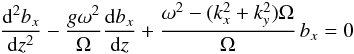 (33)with
 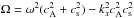 . We also obtain the relation
 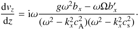 (34)This differential equation describes the propagation of ideal MHD modes. For example, inserting a solution bx = Aeikzz, we recover the well-known dispersion relation for the MHD fast and slow modes present when gravity is not taken into account. Moreover, the boundary conditions in Eqs. (32) reduce to the continuity of the normal component of the velocity perturbation and the continuity of the total pressure (plus a gravity term) by imposing ηA → 0 with the two extra conditions either identically vanishing or reducing to those; thus, they recover the ideal MHD boundary conditions.
We can study the linear phase regime of the compressible MHD RTI by solving Eq. (33). The solutions of its indicial (characteristic) equation obtained after setting bx = Aindemz (with Aind an arbitrary constant) are 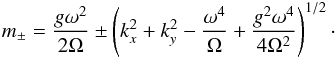 (35)We need to choose the solution in each region that guarantees the perturbation to vanish far from the discontinuity. Hence, the solution is
 ![Mathematical equation: \begin{eqnarray} b_x(z)= \left\{ \begin{array}{ll} A_{1} \, {\rm e}^{m_{1+} z}, & z < 0 , \\[3.5mm] A_{2} \, {\rm e}^{m_{2-} z}, & z > 0 , \end{array} \right. \label{mhd_sol} \end{eqnarray}](/articles/aa/full_html/2014/04/aa22147-13/aa22147-13-eq147.png) (36)with A1 and A2 being constants. Applying the remaining boundary conditions in Eq. (32), we obtain the dispersion relation for the system
(36)with A1 and A2 being constants. Applying the remaining boundary conditions in Eq. (32), we obtain the dispersion relation for the system  (37)There are a couple of interesting limiting cases to this expression. If we set g = 0, we recover the solution for surface MHD waves in an interface (see, e.g., Wentzel 1979; Roberts 1981) with no instabilities, namely
  (38)with
  . Another interesting limit is the incompressible case, which is obtained if we set csi1 → ∞ and csi2 → ∞. The dispersion relation is then
  (39)with m1 = k and m2 = −k from Eq. (35) in this limit. We can obtain an explicit equation for the frequencies of the modes,
 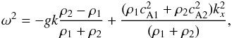 (40)which is equivalent to the classical RTI relation in Eq. (1).
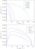 |
Fig. 2 Linear growth rate of the RTI for a fully ionized plasma (ideal MHD) as a function of the Alfvén speed |
After checking the limiting cases, we proceed to directly solve Eq. (37). The linear growth rate is plotted in Fig. 2, as compared to the predicted rate from the classical formula in Eq. (1) for the incompressible limit. The main conclusions from these results are as follows:
-
1.
The threshold is not modified by compressibility. This can beeasily demonstrated by recalling that in ideal MHD the frequencyof the modes is either real or pure imaginary (Goedbloed &Poedts 2004; Goedbloedet al. 2010), so the transition from astable to an unstable situation is necessarily at the points in whichω = 0 is satisfied. Inserting this condition in Eq. (37), we immediately recover
 (41)which matches with the stability criteria from Eq. (1) and Eq. (16). A magnetic field increase has a stabilizing effect, while increasing the angle between the equilibrium field and the wavevector has the opposite effect, as it happens in the incompressible limit.
 -
2.
The incompressible approximation becomes more valid as θ approaches π/ 2. This is caused when the incompressible limit is recovered as
 , which implies Ω → ∞, so terms containing the gravity in Eqs. (35) and (37) are negligible. We can see that increasing the longitudinal wavenumber has a similar effect in the definition of m and the dispersion relation, and hence, the incompressible limit is a better approximation as k is increased.
 -
3.
The linear growth rate for the compressible case is always below the incompressible limit prediction. As β is lowered, the linear growth rate is decreased substantially.
The curves in Fig. 2 tend to zero when the magnetic field is very low. This is caused by the choice of the sound speed: since β is fixed in these curves,  also implies that cs → 0. If the sound speed is prevented from tending to zero as B0 → 0 (implying that β is no longer held constant and tends to zero too), the drop disappears. There is also a real part of the frequency only when the configuration is stable in this ideal MHD regime, but we focus on the imaginary part and the instability. Leaky modes may also be considered (i.e., modes that propagate in the direction across the surface), but these modes do not appear for the range of parameters selected in these plots.
4.4. Partially ionized plasma
Now, we turn to the general problem with the ambipolar diffusion coefficient different from zero. Equation (29) is a fourth-order ordinary differential equation with constant coefficients, whose solutions are a combination of exponentials emkz, with mk as one of the four solutions to the indicial equation  (42)Two of these solutions are close to those in Eq. (35), while the other two are typically larger and depend strongly on the exact value of ηA. Equation (42) must be solved in each of the two regions, and then the two solutions that imply evanescence away from the discontinuity are kept. The general expression of the four roots of this fourth order algebraic equation is massive, so we choose to solve it numerically. Our general solution is then
 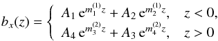 (43)with the A coefficients being arbitrary constants, the subscript of m denoting the order of the real part among the set of mk, and the superscript of m as the region where it applies.
The boundary conditions must be applied to obtain a dispersion relation, taking into account that vz must be obtained by integrating Eq. (28) after inserting the solution for bx in Eq. (43). Using the same notation in Díaz et al. (2012), the four boundary conditions are written in matricial form as ![Mathematical equation: \begin{eqnarray} \left[ \sum_{j=1,4} B_{ij} b_x^{(3-j)} \right]= 0, \label{bc_mat} \end{eqnarray}](/articles/aa/full_html/2014/04/aa22147-13/aa22147-13-eq181.png) (44)where the index i ∈ [ 1,4] stands for each boundary condition in Eqs. (32) and
(44)where the index i ∈ [ 1,4] stands for each boundary condition in Eqs. (32) and  is the j-th z-derivative of bx (j = 0 being the function itself without derivatives and j = −1 the first integral of the function). The coefficients in this matrix are given in the Appendix. Inserting the solutions from Eq. (43) in Eq. (44), we obtain a system of equations for the A-coefficients,
  (45)where the m-coefficients are defined in Eq. (42) with the requirement that the exponentials are bounded at z → ± ∞. In this expression, hk = 1 for k = 1,2, and hk = 2 for k = 3,4. The dispersion relation of the system is obtained by requiring the determinant of such system to vanish, namely
  (46)with the C-matrix defined as
  (47)The imaginary part of the solutions to Eq. (46) are plotted in Fig. 3 with the growth rates predicted by the overplotted incompressible and compressible RTI.
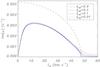 |
Fig. 3 Linear growth rate of the RTI for a partiallyl ionized plasma (taking into account ambipolar diffusion) as a function of the Alfvén speed |
The following points must be emphasized:
-
1.
A similar plot to Fig. 3 with higher values of θ would draw the collisional plasma results closer to the incompressible MHD limit and modify the critical speed. Thus, the incompressible limit is a much better approximation as θ increases, as has happened in the collisionless plasma.
-
2.
The instability threshold is no longer the one predicted by Eq. (1), namely
 km s-1 for the parameters used in the plot. The configuration is unstable for all the values of ξn and magnetic field. Considering the ambipolar term as the only effect of the presence of neutrals is enough to render this configuration (a heavier partially ionized fluid above a lighter fluid) unstable no matter how strong the magnetic field is.
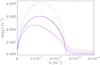
Fig. 4 Linear growth rate of the RTI for a partiallyl ionized plasma as a function of perturbation wavenumber k. The dashed line corresponds to the incompressible limit given in Eq. (1). The values ρ2/ρ1 = 100, θ = 40,
 , and ξn1 = 10-6 have been used. Solid lines are calculated with β = 0.1 and dot-dashed lines with β = 0.5, while red lines have a value for the neutral fraction ξn2 = 0.9, blue lines ξn2 = 0.5, and purple lines ξn2 = 0.1.
 -
3.
For parameters which are classically unstable (
 ), the linear growth rate is reduced a lot with respect to Eq. (1) because of the compressibility. Increasing the ambipolar coefficient slightly raises the growth rate, but the effect of the ambipolar term is small compared with compressibility in this range.
 -
4.
For parameters which are classically stable (
 ), the ambipolar diffusion still drives the instability, but the linear growth rate in this regime is an order of magnitude smaller than in the classically unstable range.
 -
5.
Close to the stability threshold (
 ), the differences induced by the ambipolar diffusion term are relatively higher.
 -
6.
In any case, the growth rate in all the parameter space is significantly lower than that of an uncoupled neutral gas that is subject to the hydrodynamic RTI (Eq. (1) with B0 = 0, ρn1 and ρn2), which would be Im[ ω] = 0.0053 s-1 for the parameters in the plot. The collisional coupling between neutrals and charged particles prevents the neutrals from fully developing their instability, even for values of ξn2 close to 1.
-
7.
As the ionization fraction is raised (and thus ξn2 and ξn1 are lowered), the curve resembles the MHD limit: there is a bifurcation very close to the critical value which can not be clearly seen in the scale of these plots and its value tends to ccrit/cos θ as the neutral fraction tends to zero.
With the inclusion of the ambipolar term, the frequencies of the modes are no longer restricted to be either pure real or pure imaginary as in the ideal MHD limit (collisionless plasma). The solutions plotted in Fig. 3 have a real conterpart Re[ ω], which are not shown in the plot. This real part is close to the compressible MHD results when  and much smaller than Im[ ω] when . We can check that there is no critical value of for which the system becomes stable: if we require ω → 0, the only real solution is ccrit = 0, confirming the numerical results in Fig. 3 and the absence of a stable region in the parameter space.
Another important parameter is the perturbation wavenumber k. So far, we have fixed a value of k = 10-7 m-1, following the typical wavenumbers from the fast transversal MHD modes of a prominence thread that was used in previous studies in prominence seismology and RTI instability in threads (Díaz et al. 2002, 2012; Terradas et al. 2012). We can further explore the effects of the initial perturbation. One important consequence is obtained after scaling the problem: it can be shown that the curves can be rescaled using the variables ω/ (ck) and  in the ideal MHD limit (with c a characteristic speed, such as Alfvén speed in the prominence, for example). This scaling involves the adimensional quantity ηAk/c if the ambipolar diffusion is included. Hence, increasing the wavenumber perturbation has the direct effect of increasing the relevance of the ambipolar term. This is expected, since it is known that the ambipolar diffusion grows as the typical length scale is reduced. On the other hand, we can also plot the linear growth rate as a function of the perturbation wavenumber (Fig. 4). We see the same main effects: there is no stable regime; the compressibility lowers the growth rate for
  , and the ambipolar diffusion slightly raises it as ξn2 is increased. It is also interesting to study this dependence near the incompressible limit with values of θ close to 90° (Fig. 5). Since compressibility is no longer dominant, the inclusion of the ambipolar term raises the growth rate over the classical RTI (as reported in Shadmehri et al. 2013 for the same assumptions that Díaz et al. 2012 uses in the context of local bubble of the solar system).
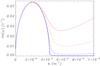 |
Fig. 5 Same plot as in Fig. 4 for the values of θ = 89 and |

Finally, we can plot the growth rate vs. the ambipolar diffusivity (Fig. 6). As mentioned above, the rate is slightly modified if the configuration is unstable in the ideal MHD limit (, upper panel) unless a very unrealistical high value of the ambipolar diffusivity is assumed. For configurations that are close to the critical value (middle panel), the dependence on the ambipolar diffusivity is more important. In the stable range (, lower panel), the linear growth rate is never zero (so strictly speaking the configuration is unstable), but the linear growth rate is at least about an order of magnitude lower than the values in classically unstable regime for typical values of ηA, so the instability would take an excessively long time to develop in practice.
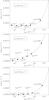 |
Fig. 6 Linear growth rate of the RTI for a partially ionized plasma as a function of the ambipolar diffusion coefficient ηA2 with some values of the neutral fraction ξn2 for which the values of ηA2 are obtained and also included in the plot as large points. The values ρ2/ρ1 = 100, β = 0.1, k = 10-7 m-1, θ = 40°, and ξn1 = 10-6 have been used (so ccrit = 47 km s-1). The upper panel corresponds to a classically unstable configuration, the middle panel to a marginally stable configuration, and the lower panel to a classically stable configuration. The dotted line in the upper panel corresponds to the MHD limit (in the middle and lower panel the classical limit is zero). |
5. Full-induction equation
We have dealt in the previous section with the effect of the induction term and the ambipolar diffusion term alone in the generalized induction equation for partially ionized plasmas (Eq. (15)). Considering only these terms has allowed us to analytically solve the linearized equations, but the effect of the other supposedly smaller terms must be taken into account. In this case, obtaining analytical solutions can be much more demanding, even in the linearized problem.
5.1. Linearized equations
In order to solve this problem, we first need to eliminate the partial pressures and the density of each species in the induction equation. This can be done by using the definition of the partial pressure pα = nαkBTα and invoking that the temperature of each species is the same (Ti = Te = Tn). Hence,  (48)and we obtain
  (49)so we can operate Eq. (9) to obtain an expression for the pressure gradients in the battery term. That is,
 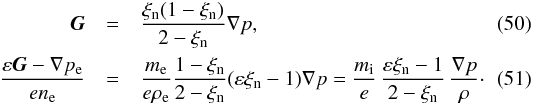 Here it is explicit that the G combination vanishes for a fully ionized plasma (ξn = 0) and the only contribution to the battery term in that case is the well-known form of the electron pressure gradient.
Next, we linearize the fluid equations. The only difference with the system in Eqs. (21) is the linear version of the induction equation. Regarding the generalized battery term, the curl of Eq. (51) is 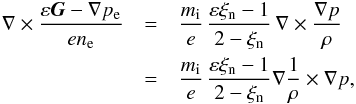 (52)and since the equilibrium state has both the density and pressure constant in each zone, this term is at least of second order for perturbed quantities and can be neglected in the linear analysis. Taking this into account the linear version of the induction equation is
 ![Mathematical equation: \begin{eqnarray} \label{lin_gen_ind} \frac{\partial {\vec b}}{\partial t} &=& \nabla \times \left( \rule{0mm}{3.5mm} {\vec v} \times {\vec B}_0 + \eta \nabla^2 {\vec b}+ \eta_\mathrm{H} \left\{ \left( \nabla \times {\vec b} \right) \times{\vec B}_0 \right\} \right. \nonumber \\ &&+ \left. \eta_\mathrm{A} \left\{ \left( \nabla \times {\vec b} \right) \times{\vec B}_0 \right\} \times{\vec B}_0 + \eta_G/(\rho_0 \cssq) \nabla p \times {\vec B}_0 \right. \nonumber \\ &&- \left. \chi_\mathrm{g1}/\rho_0 \left[ \rho_0{\vec g} \times {\vec b} + \rho \, {\vec g} \times {\vec B}_0 \right] \rule{0mm}{3.5mm} \right), \end{eqnarray}](/articles/aa/full_html/2014/04/aa22147-13/aa22147-13-eq238.png) (53)where ηA is given in Eq. (26) and the other diffusion coefficients can be also expressed in terms of the ionization fraction and the equilibrium parameters,
(53)where ηA is given in Eq. (26) and the other diffusion coefficients can be also expressed in terms of the ionization fraction and the equilibrium parameters, ![Mathematical equation: \begin{eqnarray} \eta &=& \frac{m_{\rm i} m_{\rm e}}{\mu {\rm e}^2} \frac{1}{\rho_0 (1- \xi_{\rm n})} \left[ \nu_{\rm en} (\xi_{\rm n}) + \nu_{\rm ei} (\xi_{\rm n}) \right] - \frac{m_{\rm e}^2}{\mu {\rm e}^2} \frac{(\nu_{\rm en} (\xi_{\rm n}))^2}{\alpha_{\rm n} (\xi_{\rm n})}, \nonumber \\ \eta_\mathrm{H} &=& \frac{m_{\rm i}}{\mu e} \frac{1}{\rho_0 (1-\xi_{\rm n})} \left[1 - \frac{\sqrt{2}}{5} \frac{m_{\rm e}}{m_{\rm i}} \xi_{\rm n} \right] , \nonumber \\ \chi_\mathrm{G} &=& \rho_0 \cssq \frac{\xi_{\rm n}^2}{\alpha_{\rm n}} \, \frac{1-\xi_{\rm n}}{2-\xi_{\rm n}}, \nonumber \\ \chi_\mathrm{g1} &=& \rho_0 \frac{\xi_{\rm n}^2}{\alpha_{\rm n}} \frac{m_{\rm e}}{m_{\rm i}} (1-\xi_{\rm n}). \end{eqnarray}](/articles/aa/full_html/2014/04/aa22147-13/aa22147-13-eq239.png) (54)Eliminating the perturbed pressure and density, we obtain the following set of partial differential equations for the components of the perturbed velocity and magnetic field,
(54)Eliminating the perturbed pressure and density, we obtain the following set of partial differential equations for the components of the perturbed velocity and magnetic field, ![Mathematical equation: \begin{eqnarray} \frac{\partial^2 {\vec v}}{\partial t^2} &=& \frac{1}{\mu \rho_0} \left(\nabla \times {\vec b} \right) \times {\vec B}_0 - \left(\nabla \cdot {\vec v}\right) {\vec g} + \cssq \nabla \left( \nabla \cdot {\vec v} \right), \nonumber \\ \frac{\partial^2 {\vec b}}{\partial t^2} &=& \nabla \times \left( \frac{\partial {\vec v}}{\partial t} \times {\vec B}_0 \right) + \eta \nabla^2 \frac{\partial {\vec b}}{\partial t} \nonumber \\ &&- \eta_\mathrm{H} \nabla \times \left\{ \left( \nabla \times \frac{\partial {\vec b}}{\partial t} \right) \times{\vec B}_0 \right\} \nonumber \\ &&+ \eta_\mathrm{A} \left\{ \left( \nabla \times \frac{\partial {\vec b}} {\partial t}\right) \times{\vec B}_0 \right\} \times{\vec B}_0 \nonumber \\ &&+ \chi_\mathrm{G} \nabla \times \left\{ \nabla (\nabla \cdot {\vec v}) \times {\vec B}_0 \right\} \nonumber \\ &&+ \chi_\mathrm{g1} \left[ \left\{ \nabla (\nabla \cdot {\vec v} )\right\} \times \left( {\vec g} \times {\vec B}_0 \right) - \left( {\vec g} \cdot \nabla \right) \frac{\partial {\vec b}} {\partial t} \right]\cdot \label{linear_eqs2} \end{eqnarray}](/articles/aa/full_html/2014/04/aa22147-13/aa22147-13-eq240.png) (55)The complexity of these equations is evident, and even third order derivatives are present in the term coming from G × B. Finding direct analytical solutions is still possible in our problem if we notice that all the coefficients are constant in each region of our model, so we obtain a third order linear system of six equations, whose solutions are written in terms of linear combinations of exponential functions.
(55)The complexity of these equations is evident, and even third order derivatives are present in the term coming from G × B. Finding direct analytical solutions is still possible in our problem if we notice that all the coefficients are constant in each region of our model, so we obtain a third order linear system of six equations, whose solutions are written in terms of linear combinations of exponential functions.
5.2. Normal mode analysis
We again consider the normal mode decomposition with the temporal dependence when e− iωt and the dependence on the directions where the equilibrium state is uniform when eikxx + ikyy. Now we can eliminate vx, vy, and bz to obtain the three differential equations, which are given in the Appendix. We obtain four solutions that go to zero as z → ∞ and another four that go to zero as z → − ∞, so the general solution in each zone would be a linear combination of the four linearly independent solutions that satisfy the boundary condition as | z | → ∞ in each region.
Next, we need to derive the boundary conditions appropiate to this problem, and following the procedure used in the case of ambipolar diffusion alone, we go directly to Eqs. (55) and integrate them across the boundary, obtaining only five relations between the variables ![Mathematical equation: \begin{eqnarray} \label{bc1} &&\left[ \rho_0 \cssq v_z \right] = 0, \nonumber \\ &&\left[ \rho_0 \left\{ {\rm i} \omega c_\mathrm{A}^2 b_x c_\mathrm{s} - {\rm i}k_x c_\mathrm{s}^2 v_x - {\rm i}k_y c_\mathrm{s}^2 v_y - g v_z + c_\mathrm{s}^2 v_z' \right\} \right] =0, \nonumber \\ &&\left[ \eta_\mathrm{A} ({\rm i} k_x \omega b_z + \omega b_x') -\eta \omega b_x' -{\rm i} k_x \omega b_y \eta_\mathrm{H} \right. \nonumber \\ && \qquad\qquad\quad \left. + \,\chi_\mathrm{G} c_\mathrm{s}^2 (-{\rm i} k_y^2 v_z + k_x v_x'+k_y v_y' + {\rm i}v_z'') \right. \nonumber \\ && \qquad\qquad\quad \left. -\,g \chi_\mathrm{g1} (\omega b_x + k_x v_x +k_y v_y + {\rm i}v_z') - \omega v_z \right] = 0, \nonumber \\ &&\left[ {\rm i}k_x \left( \omega b_x \eta_\mathrm{H} +k_y c_\mathrm{s}^3 \chi_\mathrm{G} v_z \right) -\omega \eta b_y' -g \omega b_y \chi_\mathrm{g1} \right] =0, \nonumber \\ &&\left[ k_x \omega \eta_\mathrm{A} b_x +{\rm i} \omega \eta b_z'- {\rm i}g k_x c_\mathrm{s} \chi_\mathrm{g1} v_z \right. \nonumber \\ && \qquad\qquad\quad \left. +\,k_x c_\mathrm{s}^3 \chi_\mathrm{G} \left(k_x v_x +k_y v_y +{\rm i} v_z' \right) \right] = 0. \end{eqnarray}](/articles/aa/full_html/2014/04/aa22147-13/aa22147-13-eq247.png) (56)However, these relations are not enough for our problem, which has four arbitrary constants in each side of the boundary. The divergence-free condition ∇·b = 0 and the expressions for the perturbed pressure and density in Eqs. (21) only give us linear combinations of the conditions in Eq. (56). To obtain the additional relations, we need to use the equation for the diffusion velocity between ions and neutrals (which introduces the higher-order derivatives in the linearized equations). The linear version of Eq. (11) is
(56)However, these relations are not enough for our problem, which has four arbitrary constants in each side of the boundary. The divergence-free condition ∇·b = 0 and the expressions for the perturbed pressure and density in Eqs. (21) only give us linear combinations of the conditions in Eq. (56). To obtain the additional relations, we need to use the equation for the diffusion velocity between ions and neutrals (which introduces the higher-order derivatives in the linearized equations). The linear version of Eq. (11) is ![Mathematical equation: \begin{eqnarray} {\vec w} &=& \eta_\mathrm{A} \left[ \nabla \times \frac{\partial {\vec b}}{\partial t} \right] \times {\vec B}_0 + \chi_\mathrm{G1} \nabla \left( \nabla \cdot {\vec v} \right) \nonumber \\ &&+ \eta_\mathrm{H1} \nabla \times \frac{\partial {\vec b}}{\partial t} - \chi_\mathrm{g2} (\nabla \cdot {\vec v}) \, {\vec g} =0 \end{eqnarray}](/articles/aa/full_html/2014/04/aa22147-13/aa22147-13-eq249.png) (57)with the coefficients defined as
(57)with the coefficients defined as 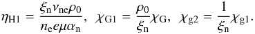 (58)Using this equation, we obtain the remaining three jump relations for our system, namely
 ![Mathematical equation: \begin{eqnarray} \label{bc2} &&\left[ \alpha_{\rm n} \left( \omega b_y \eta_\mathrm{H1} -{\rm i} k_x c_\mathrm{s} \chi_\mathrm{G1} v_z \right) \right] = 0, \nonumber \\ &&\left[ \alpha_{\rm n} \left( -{\rm i} \omega b_x \eta_\mathrm{H1}- {\rm i}k_y c_\mathrm{s} \chi_\mathrm{G1} v_z \right)\right]= 0, \nonumber \\ &&\left[ \alpha_{\rm n} \left( {\rm i} \omega \eta_\mathrm{A} b_x - g c_\mathrm{s} \chi_\mathrm{g2} v_z -{\rm i} k_x c_\mathrm{s} \chi_\mathrm{G1} v_x\right. \right. \nonumber \\ && \left. \rule{0mm}{3.5mm} \left.- {\rm i}k_y c_\mathrm{s} \chi_\mathrm{G1} v_y +c_\mathrm{s} \chi_\mathrm{G1} v_z' \right) \right] = 0, \end{eqnarray}](/articles/aa/full_html/2014/04/aa22147-13/aa22147-13-eq251.png) (59)which provides us with the remaining conditions to solve the linear problem. Notice that we easily recover the case with ambipolar diffusion alone, since the first two equations vanish in this case and the last one becomes equivalent to the last jump condition in Eq. (31).
(59)which provides us with the remaining conditions to solve the linear problem. Notice that we easily recover the case with ambipolar diffusion alone, since the first two equations vanish in this case and the last one becomes equivalent to the last jump condition in Eq. (31).
5.3. Numerical solutions
The solution of the problem must be computed in the following form: first of all, the differential equations in Eq. (A.3) for bx, by, and vz must be solved in each zone by obtaining the set of solutions for λ from Eq. (A.6) (and the relation between the constants of each variable), and then discarding the solutions that do not vanish as | z | → 0. This leaves us with solutions with four arbitrary constants in each zone. Finally, the jump conditions in Eqs. (56) and (59) must be satisfied, which can only be achieved if the determinant of the system of this eight equation vanishes. This provides us with a dispersion relation for computing the frequencies of our system and, thus studies the stability of the system by checking if their imaginary parts are either positive (unstable modes) or negative (stable modes).
The procedure described in the previous paragraph does not give simple analytical solutions, so we use it to find numerical solutions to the system. It is important to remark that these solutions are not obtained from partial differential equations but from an algebraic system of equations. There is a huge range of parameters that can be explored, but we concentrate here on the situations of physical interest for the RTI instability, namely, when all the diffusive terms are much lower than the induction term. All the η and χ coefficients in these diffusive terms depend on the ionization fraction ξn due to their dependence on the densities, collisions frequencies, and temperatures.
First of all, we study the numerical values and dependence of the different collision frequencies, since we also need the collisional frequencies of electrons with other species, which are (Soler et al. 2009; Braginskii 1965) 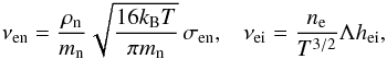 (60)where σen ≈ 10-19 m2, hei ≈ 3.7 × 10⁻⁶ s-1 m-3 K3/2, and Λ is the Coulomb logarithm. We plot these frequencies in terms of the ionization fraction in Fig. 7 for values of the parameters typical in prominences, namely ρ0 = 10-10 kg m-3, p0 = 0.135 Pa, and B0 = 10 G, so cs = 15 km s-1 and cA = 89 km s-1. For fully ionized plasmas, the neutral collision frequencies vanish, as expected, but it becomes comparable and even larger than the collision frequency between ions and electrons as the ionization fraction is increased. Note that the assumption in Soler et al. (2012b), Díaz et al. (2012) of neglecting the electron collisions might not be appropiate for these values of the plasma parameters (specially for low values of ξn).
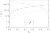 |
Fig. 7 Collisional frequencies as a function of the ionization fraction for the values of the density, pressure, and magnetic field given in the text. |
Regarding the different terms in the linealized induction equation (Eq. (55)), the values of each term are represented in Fig. 8 for typical values of kx = ky = 10-7 m-1, g = 270 m s-1, and Im[ ω] ≈ 0.007 s-1, which are normalized to the magnitude of the ideal MHD induction term ∇ × (v × B0). The dominant term under these plasma conditions is the ambipolar term, which was studied independently in the previous section. Then, the Hall and perpendicular battery terms are typically about one order of magnitude smaller than the ambipolar, and finally, the gravity and ohmic diffusion terms are much lower. Note that the ambipolar, battery, and gravity terms tend to zero for a fully ionized plasma ξn → 0, but the hall and ohmic terms are still present. In addition, the battery term neglected in the linearization (Eq. (51)) would also be present for a fully ionized plasma.
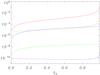 |
Fig. 8 Numerical values of the terms in the induction equation in Eq. (55) relative to the ideal MHD term with the values stated in the text. The red line corresponds to the ambipolar term, the blue line to the Hall term, the orange line to the perpendicular battery term (G × B), the green line to the gravity terms and the purple line to the Ohmic term. |
Next, we study the solutions of the indicial equation (Eq. (A.6)). There are four solutions that are very close to the ones in Eq. (42), and four new ones that are related to the other diffusion coefficients. These are about four orders of magnitude larger (and thus describe only diffusive effects very near the boundary and are negligible far from it). However, these diffusive solutions are troublesome from the computational point of view, since they introduce large coefficients in the boundary conditions that must be computed with great accuracy.
Finally, we can obtain the frequency of the modes of the system. We concentrate on the relevant modes to the stability analysis. The imaginary part of the frequency is plotted near the instability threshold in Fig. 9 for a typical set of parameters in the prominence thread oscillations. The differences between the ambipolar result and the full equations are small, but one interesting difference is that the inclusion of the rest of the terms in the induction equation raises the linear growth rate slightly in the MHD stable regime (which corresponds to kx> 1.3 × 10⁻⁷ m-1 for these parameters). In the MHD unstable regime (kx< 1.3 × 10⁻⁷ m-1), it lowers it slightly, but the corrections are small compared with the computed values for the ambipolar case. Hence, as expected from Fig. 8, the rest of the terms offer just slight corrections to the results for the ambipolar case described in Sect. 4, at least for the physical and plasma parameters in prominences.
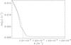 |
Fig. 9 Linear growth rate of the RTI as a function of the wavenumber. The values chosen for the plot are ρ2 = 10-10 kg m-3, ρ2/ρ1 = 100, θ = 85° m-1, B0 = 10 G, cs2 = 15 km s-1, ξ2 = 0.5, and ξ1 = 0.1. The dashed line is the incompressible MHD limit from Eq. (1); the dotted line corresponds to the PI one-fluid model with only the ambipolar term (Sect. 4); and the solid line to the PI one-fluid model with all the terms in the induction equation. |
It is very interesting to notice that the PI effects do not qualitatively modify the linear growth rate in the region of classical stability. This is in contradiction with the result in Díaz et al. (2012), who reported that the linear growth rate was lowered by an order of magnitude in their Sect. 5. However, a very low value of the equilibrium density was chosen to compute νin in that calculation, so it would correspond to the case in which the ambipolar coefficient is chosen to be larger than the value obtained in this work. We can see in Fig. 9 that the effects of PI do not lower that drastically the linear growth rate for this set of parameters. We obtain a typical RTI timescale of about 100 s from Fig. 9, similar to the lifetime of prominence threads (Labrosse et al. 2010; Mackay et al. 2010; Lin 2011).
6. Discussion and conclusions
We have studied the effects of considering a partially ionized plasma in the MHD Rayleigh-Taylor instability in a contact surface where a heavier plasma sits on top of a lighter one. We have simplified considerably the problem by assuming that the equilibrium variables are uniform in each region, which is only valid if the vertical scales of the perturbations are much smaller than the gravitational scale height. In the initial stages of the instability, the solution is confined to the boundary, so this approximation is useful. However, the gravity stratification may become important in later stages, but then the differential equations may become too hard to be solved analytically. The problem is better posed in terms of numerical studies, which would also allow us to characterize the non-linear phases of the instability.
Including PI effects in the MHD equations can be done in several ways. In Díaz et al. (2012), a two-fluid model was considered with only the collisions between ions and neutrals as deemed important. Here, we have taken a different approach by using all the collision frequencies between the species, but we combine the fluid equations for each species into one-fluid equations (following Braginskii 1965, for example). These PI effects then appear in the form of a generalized Ohm’s law (Eq. (12)) and an induction equation (Eq. (13)) with the corresponding terms in the energy equation (which are second order effects in the linear analysis). We follow the standard procedure of deriving a relation for the diffusion velocity between ions and neutrals from the equation of motion for electrons (with the electron inertial terms neglected). However, in contrast with previous deductions, we have kept all the terms, by obtaining the well known expressions for the ohmic, ambipolar, Hall, and battery diffusion terms but also for the G × B (similar to the Hall term with diamagnetic currents) and the gravity term. This gravity effect has been normally overlooked, because it comes from neglecting the electron gravity force in front of the ion gravity force on the combined momentum equation for ions and electrons. However, we have proved that this term survives as the equation for the diffusion velocity is obtained. Under prominence thread circumstances, this term is nevertheless small but can be still larger than the ohmic diffusion and might also be relevant in other contexts.
It has been previously assessed that the most important term in the generalized Ohm’s law is the ambipolar diffusion term (Khomenko & Collados 2012). We first study the modifications that this term implies in the linear regime. An ordinary differential equation is derived with constant coefficients because of the uniform plasma assumption in each zone, so a solution close to the ideal MHD is found with another related to the ambipolar coefficient. The ordinary MHD jump relations are not enough, so we derive our boundary relations directly from the differential equations by following Chandrasekhar (1961). We then obtain new conditions to add to the continuity of total pressure are perpendicular velocity. Finally, the modes of the system are obtained with the MHD limit recovered when ηA → 0. The main conclusion is that the configuration is always unstable, regardless of the values of the parameters. In the region of the parameter space where there was classical stability, the linear growth rate is very small, while the ambipolar diffusion slightly raises the linear growth rate compared with the compressible MHD limit in the classically stable region. These results support the conclusions in Díaz et al. (2012), and both descriptions qualitatively agree despite considering different assumptions on the fluid equations. Notice, however, that Díaz et al. (2012) considered that the collision frequency of both media were simply related by ρ2/ρ1 in the two-fluid description and used a high value of equilibrium density, while we have derived a relation between the ambipolar diffusion coefficients in both regions by considering all the dependence of the equilibrium parameters on ξn in both regions here.
Next, we consider the full induction equation. We check first the relevance of the different terms in the linear analysis. It is found that the battery and gravity terms do not give any direct contribution in the linear regime in a uniform equilibrium medium, but their Hall counterparts still appear. The other terms are orders of magnitude smaller than the ambipolar term. The problem is solved in a similar way with extra solutions to the indicial equation because of these dissipative terms. The numerical analysis of the solutions confirms that they only induce small corrections to the results of the ambipolar case for typical values of prominence threads.
A direct application of the results of this paper concerns solar prominence threads. It is widely assumed that chromospheric material sits on top of a less dense coronal plasma in either a static equilibrium or dynamical configurations. The RTI has been studied numerically in such configurations (Hillier et al. 2011, 2012a). It is interesting to test the differences that PI effects produce, especially when we consider that the material that forms the prominence is expected to be partially ionized (despite the ionization fraction has not been directly measured so far). A plot of the linear growth rate for different values of the equilibrium field is displayed in Fig. 10. The effects described in our analysis can be summarized as follows:
-
There is no critical value: the configuration is always unstable tothe RTI instability because of the presence of neutrals.
-
In the region of classical stability, the PI terms give a small linear growth rate, so the time scale of the instability is much larger than the typical lifetime of the threads.
-
On the region of classical instability, the PI also affects the growth rate, but this rate is still very high (despite a stabilizing effect of the compressibility), so the RTI is very efficient and can disrupt the threads.
-
For typical prominence plasma parameters, the PI effects are small, since the ambipolar term is much smaller than the MHD induction term (Fig. 8) and the perturbation is nearly incompressible (Terradas et al. 2012). However, the effect becomes more pronounced if the term is larger than the theoretical values. This can be seen in the plot for a high ηA value in Fig. 10.
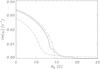
Fig. 10 Linear growth rate vs. equilibrium magnetic field for ρ2/ρ1 = 100, g = 270 m s-2, θ = 87°, k = 5 × 10⁻⁶ m-1, ξn1 = 10-4, and ρ2 = 10-10 kg m-3. The dotted line is the ambipolar case with ξn2 = 0.5, the solid line with ξn2 = 0.05 and the dot-dashed line to ξn2 = 0.5 but with a value for the ambipolar diffusion coefficient that is 1000 times larger than the theoretical value used in the rest of the computations. The dashed line corresponds to the incompressible MHD limit (Eq. (1)).
-
The leading ambipolar term becomes important on small scales (for typical prominence parameters, whose scales are expected to be in the range of 100 km and below). Current observational facilities are almost at this limit, like the Japanese HINODE mission (Tsuneta et al. 2008) or the Sunrise/IMaX instrument (Martínez Pillet et al. 2011), and the new generation of telescopes, such as EST (Collados et al. 2013) or ATST (Keil et al. 2011), are aimed to provide information on such scales. Thus, we are about to be able to observe the spatial range where the PI effects in prominences might be directly observed.
-
Including other additional PI terms beyond the leading ambipolar term only give small numerical changes (mainly near the classical critical value) at the price of a much harder analytical and computational effort.
These conclusions need to be tested in several ways. First of all, the analysis carried out in this work is only valid in the linear regime. Once the instability is triggered on, non-linearities may become important, and it is well-known from MHD simulations that secondary Kelvin-Hemholtz instabilities appear (seen as eddies in the simulations) once the stability is well developed. The linear growth rate is therefore lowered and the drops formed reach a terminal velocity; all these processes are not present in the linear analysis. Moreover, the battery term contribution can be neglected in the linear analysis but helps to raise currents in the non-linear regime. More crucially, no new effects are present in the linearized energy equation.
Another neglected effect that might be important is the presence of a density stratification (mainly due to gravity), despite having typical length scales much larger than the thread thickness. Some studies point out that these stratification effects have a stabilizing contribution on the RTI (Liberatore et al. 2009). However, considering a non-uniform plasma in each region complicates substantially the analysis (especially the differential equations, which no longer have constant coefficients) and might change the relevance of some terms (such as the battery term, which would have a linear contribution). In this case, the problem is better posed to numerical solutions, especially considering that other effects might also be important, such as the curvature of the field lines forming the dip that sustains the condensation, which constitutes the thread.
Numerical simulations are underway to study the complex effects of PI in the instability and the non-linear regime (Khomenko et al. 2013). The calculations in this work offer a guide to test the results at least in the first stages of the instability.
Acknowledgments
The authors acknowledge the financial support by the Spanish Ministry of Science through project AYA2010-18029. This work contributes to the deliverables identified in FP7 European Research Council grant agreement 277829, “Magnetic connectivity through the Solar Partially Ionized Atmosphere”, whose PI is E. Khomenko (Milestone 3 and contribution toward Milestones 1).
References
- Arber, T. D., Haynes, M., & Leake, J. E. 2007, ApJ, 666, 541 [NASA ADS] [CrossRef] [Google Scholar]
- Balescu, R. 1988, Transport processes in a plasma (North Holland: Amsterdam) [Google Scholar]
- Berger, T. E., Shine, R. A., Slater, G. L., et al. 2008, ApJ, 676, L89 [Google Scholar]
- Berger, T. E., Slater, G., Hurlburt, N., et al. 2010, ApJ, 716, 1288 [NASA ADS] [CrossRef] [Google Scholar]
- Berger, T., Testa, P., Hillier, A., et al. 2011, Nature, 472, 197 [NASA ADS] [CrossRef] [PubMed] [Google Scholar]
- Bernstein, I. B., & Book, D. L. 1983, Phys. Fluids, 26, 453 [NASA ADS] [CrossRef] [Google Scholar]
- Bittencourt, J. A. 1986, Fundamentals of plasma physics (Oxford: Pergamon Press) [Google Scholar]
- Braginskii, S. I. 1965, Transport Processes in Plasma, ed. M. A. Leontovich (New York, USA: Consultants Bureau), 201 [Google Scholar]
- Breitschwerdt, D., Freyberg, M. J., & Egger, R. 2000, A&A, 361, 303 [NASA ADS] [Google Scholar]
- Bucciantini, N., Amato, E., Bandiera, R., Blondin, J. M., & Del Zanna, L. 2004, A&A, 423, 253 [NASA ADS] [CrossRef] [EDP Sciences] [Google Scholar]
- Chandrasekhar, S. 1961, Hydrodynamic and Hydromagnetic Stability (CUP, New York: Dover Publications Inc.) [Google Scholar]
- Chhajlani, R. K., & Vaghela, D. S. 1989, Ap&SS, 155, 257 [NASA ADS] [CrossRef] [Google Scholar]
- Collados, M., Bettonvil, F., Cavaller, L., et al. 2013, Mem. Soc. Astron. Italiana, 84, 379 [Google Scholar]
- Díaz, A. J., Oliver, R., & Ballester, J. L. 2002, ApJ, 580, 550 [NASA ADS] [CrossRef] [Google Scholar]
- Díaz, A. J., Soler, R., & Ballester, J. L. 2012, ApJ, 754, 41 [NASA ADS] [CrossRef] [Google Scholar]
- Drazin, P. G., & Reid, W. H. 1981, Hydrodynamic stability (Cambridge Mathematical Library), 82, 17950 [Google Scholar]
- Eggleton, P. P., Dearborn, D. S. P., & Lattanzio, J. C. 2006, Science, 314, 1580 [NASA ADS] [CrossRef] [PubMed] [Google Scholar]
- Forteza, P., Oliver, R., Ballester, J. L., & Khodachenko, M. L. 2007, A&A, 461, 731 [NASA ADS] [CrossRef] [EDP Sciences] [Google Scholar]
- Fryxell, B., Arnett, D., & Mueller, E. 1991, ApJ, 367, 619 [NASA ADS] [CrossRef] [Google Scholar]
- Gilbert, H., Kilper, G., & Alexander, D. 2007, ApJ, 671, 978 [NASA ADS] [CrossRef] [Google Scholar]
- Goedbloed, J. P. H., Keppens, R., & Poedts, S. 2010, Advanced Magnetohydrodynamics (Cambridge) [Google Scholar]
- Goedbloed, J. P. H., & Poedts, S. 2004, Principles of Magnetohydrodynamics (Cambridge) [Google Scholar]
- Heinzel, P., Schmieder, B., Fárník, F., et al. 2008, ApJ, 686, 1383 [NASA ADS] [CrossRef] [Google Scholar]
- Hillier, A., Isobe, H., Shibata, K., & Berger, T. 2011, ApJ, 736, L1 [NASA ADS] [CrossRef] [Google Scholar]
- Hillier, A., Berger, T., Isobe, H., & Shibata, K. 2012a, ApJ, 746, 120 [NASA ADS] [CrossRef] [Google Scholar]
- Hillier, A., Hillier, R., & Tripathi, D. 2012b, ApJ, 761, 106 [NASA ADS] [CrossRef] [Google Scholar]
- Hillier, A., Isobe, H., Shibata, K., & Berger, T. 2012c, ApJ, 756, 110 [NASA ADS] [CrossRef] [Google Scholar]
- Isobe, H., Miyagoshi, T., Shibata, K., & Yokoyama, T. 2005, Nature, 434, 478 [NASA ADS] [CrossRef] [Google Scholar]
- Isobe, H., Miyagoshi, T., Shibata, K., & Yokoyama, T. 2006, PASJ, 58, 423 [Google Scholar]
- Jun, B.-I., Norman, M. L., & Stone, J. M. 1995, ApJ, 453, 332 [NASA ADS] [CrossRef] [Google Scholar]
- Keil, S. L., Rimmele, T. R., Wagner, J., Elmore, D., & ATST Team. 2011, in Solar Polarization 6, eds. J. R. Kuhn, D. M. Harrington, H. Lin, et al., ASP Conf. Ser., 437, 319 [Google Scholar]
- Khodachenko, M. L., Arber, T. D., Rucker, H. O., & Hanslmeier, A. 2004, A&A, 422, 1073 [NASA ADS] [CrossRef] [EDP Sciences] [Google Scholar]
- Khomenko, E., & Collados, M. 2012, ApJ, 747, 87 [NASA ADS] [CrossRef] [Google Scholar]
- Khomenko, E., Díaz, A. J., Collados, M., & De Vicente, A. 2013, A&A, in press [Google Scholar]
- Labrosse, N., Heinzel, P., Vial, J.-C., et al. 2010, Space Sci. Rev., 151, 243 [Google Scholar]
- Liberatore, S., & Bouquet, S. 2008, Phys. Fluids, 20, 116101 [NASA ADS] [CrossRef] [Google Scholar]
- Liberatore, S., Jaouen, S., Tabakhoff, E., & Canaud, B. 2009, Phys. Plasmas, 16, 044502 [NASA ADS] [CrossRef] [Google Scholar]
- Lin, Y. 2011, Space Sci. Rev., 158, 237 [NASA ADS] [CrossRef] [Google Scholar]
- Livescu, D. 2004, Phys. Fluids, 16, 118 [NASA ADS] [CrossRef] [MathSciNet] [Google Scholar]
- Mackay, D. H., Karpen, J. T., Ballester, J. L., Schmieder, B., & Aulanier, G. 2010, Space Sci. Rev., 151, 333 [NASA ADS] [CrossRef] [Google Scholar]
- Martínez Pillet, V., Del Toro Iniesta, J. C., Álvarez-Herrero, A., et al. 2011, Sol. Phys., 268, 57 [NASA ADS] [CrossRef] [Google Scholar]
- Matsumoto, J., & Masada, Y. 2013, ApJ, 772, L1 [NASA ADS] [CrossRef] [Google Scholar]
- Mitchner, M., & Kruger, C. H. 1973, Partially Ionized Gases (New York: John Wiley and Sons) [Google Scholar]
- Parker, E. N. 1979, Ap&SS, 62, 135 [NASA ADS] [Google Scholar]
- Patsourakos, S., & Vial, J.-C. 2002, Sol. Phys., 208, 253 [NASA ADS] [CrossRef] [Google Scholar]
- Priest, E. R. 1982, Solar Magnetohydrodynamics (D. Reidel Publishing Company) [Google Scholar]
- Ribeyre, X., Tikhonchuk, V. T., & Bouquet, S. 2004, Phys. Fluids, 16, 4661 [NASA ADS] [CrossRef] [Google Scholar]
- Roberts, B. 1981, Sol. Phys., 69, 27 [NASA ADS] [CrossRef] [Google Scholar]
- Ryutova, M., Berger, T., Frank, Z., Tarbell, T., & Title, A. 2010, Sol. Phys., 267, 75 [Google Scholar]
- Shadmehri, M., Yaghoobi, A., & Khajavi, M. 2013, Ap&SS [arXiv:1305.2475] [Google Scholar]
- Shivamoggi, B. K. 1982, Phys. Fluids, 25, 911 [NASA ADS] [CrossRef] [Google Scholar]
- Shivamoggi, B. K. 2008 [Google Scholar]
- Soler, R., Oliver, R., & Ballester, J. L. 2009, ApJ, 699, 1553 [NASA ADS] [CrossRef] [Google Scholar]
- Soler, R., Andries, J., & Goossens, M. 2012a, A&A, 537, A84 [NASA ADS] [CrossRef] [EDP Sciences] [Google Scholar]
- Soler, R., Diaz, A. J., Ballester, J. L., & Goossens, M. 2012b, ApJ, 749, 163 [NASA ADS] [CrossRef] [Google Scholar]
- Stone, J. M., & Gardiner, T. 2007, ApJ, 671, 1726 [NASA ADS] [CrossRef] [Google Scholar]
- Terradas, J., Oliver, R., & Ballester, J. L. 2012, A&A, 541, A102 [NASA ADS] [CrossRef] [EDP Sciences] [Google Scholar]
- Tsuneta, S., Ichimoto, K., Katsukawa, Y., et al. 2008, Sol. Phys., 249, 167 [NASA ADS] [CrossRef] [Google Scholar]
- Vandervoort, P. O. 1961, AJ, 66, 56 [Google Scholar]
- Vranjes, J., & Krstic, P. S. 2013, A&A, 544, A22 [NASA ADS] [CrossRef] [EDP Sciences] [Google Scholar]
- Wang, Y.-M., & Nepveu, M. 1983, A&A, 118, 267 [NASA ADS] [Google Scholar]
- Wentzel, D. G. 1979, ApJ, 227, 319 [NASA ADS] [CrossRef] [Google Scholar]
- Zaqarashvili, T. V., Khodachenko, M. L., & Rucker, H. O. 2011a, A&A, 534, A93 [NASA ADS] [CrossRef] [EDP Sciences] [Google Scholar]
- Zaqarashvili, T. V., Khodachenko, M. L., & Rucker, H. O. 2011b, A&A, 529, A82 [NASA ADS] [CrossRef] [EDP Sciences] [Google Scholar]
Appendix A: Coefficients on the linear system of equations
Here, we present the coefficients that appear in the linearized equations for both the ambipolar diffusion section and the general case. If only ambipolar diffusion is considered in the induction equation (Sect. 4), then the boundary conditions can be written in terms of bx, as is shown in Eq. (44). ![Mathematical equation: \appendix \setcounter{section}{1} \begin{eqnarray} B_{11} &\,=\,& 0, \nonumber \\ B_{12} &\,=\,& \left\{ {\rm i} (\omega + {\rm i} k_x^2 \etaa)[-k^2 \casq (\omega^2 - k_x^2 \cssq) \right. \nonumber \\ &&+ \left. \omega (\omega^2 - k^2 \cssq) (\omega + k^2 \etaa)]\right\}/\left\{ (\omega^2-k_x^2 \cssq) (\omega^2 \right. \nonumber \\ &&- \left. k_x^2 \casq + {\rm i} \omega \etaa k_x^2)\right\}, \nonumber \\ B_{13} &\,=\,& 0, \nonumber \\ B_{14} &\,=\,& \etaa \frac{-k_x^2 \casq(\omega^2-k_x^2 \cssq)+ \omega (\omega^2 - k^2 \cssq)(\omega + {\rm i} k_x^2 \etaa)}{(\omega^2 - k_x^2 \cssq)(\omega^2 - k_x^2 \casq + {\rm i} \omega \etaa k_x^2)}, \nonumber \\ B_{21} &\,=\,& \frac{\omega^2 \cssq \etaa}{\omega^2-k_x^2 \cssq}, \nonumber \\ B_{22} &\,=\,& g \etaa \frac{k_x^2 \casq (\omega^2-k_x^2 \cssq) - \omega (\omega^2 - k^2 \cssq) (\omega + {\rm i} k_x^2 \etaa)} {(\omega^2-k_x^2 \cssq)(\omega^2 - k_x^2 \casq + {\rm i} \omega \etaa k_x^2)} , \nonumber \\ B_{23} &\,=\,& {\rm i} \omega \frac{\omega^2 (\casq+\cssq) + {\rm i} \omega k^2 \cssq \etaa -k_x^2 \casq \cssq}{\omega^2-k_x^2 \cssq}, \nonumber \\ B_{24} &\,=\,& - g ({\rm i}\omega - k_x^2 \etaa) \times \nonumber \\ && \frac{- k^2 \casq (\omega^2 - k_x^2 \cssq) + \omega (\omega^2 - k^2 \cssq) (\omega + {\rm i} k^2 \etaa)}{(\omega^2-k_x^2 \cssq)(\omega^2 - k_x^2 \casq + {\rm i} \omega \etaa k_x^2)}, \nonumber \\ B_{31} &\,=\,& 0, \nonumber \\ B_{32} &\,=\,& \frac{k_y^2 \omega \cssq \etaa}{(\omega^2 - k_x^2 \cssq) (\omega^2 - k_x^2 \casq + {\rm i} \omega \etaa k_x^2)}, \nonumber \\ B_{33} &\,=\,& 0, \nonumber \end{eqnarray}](/articles/aa/full_html/2014/04/aa22147-13/aa22147-13-eq284.png)
 (A.1)These coefficients are then used in Eq. (47) to compute the growth rates.
Next, we present the coefficients that appear in the linearized equations for the general case, when all the terms in the induction equation are considered (Sect. 5). The method is similar to the one applied in the ambipolar case, but the complexity of the problem prevents us from writing the boundary conditions in terms of a single magnitude, as it was done in the ambipolar section using bx. First of all, we express vx, vy, and bz from the linearized equation of motion (Eq. (53)) as follows ![Mathematical equation: \appendix \setcounter{section}{1} \begin{eqnarray} v_x &\,=\,& \frac{k_x c_\mathrm{s} \left(k_y c_\mathrm{A}^2 (k_x b_y -k_y b_x)+ {\rm i} \omega c_\mathrm{s} v_z' \right)}{\omega^3- \omega c_\mathrm{s}^2 \left(k_x^2+k_y^2\right)}, \nonumber \\[0.6mm] v_y &\,=\,& \frac{c_\mathrm{A}^2 \left(k_x^2 c_\mathrm{s}^2-\omega^2\right) (k_y b_x-k_x b_y)+ {\rm i} k_y \omega c_\mathrm{s}^3 v_z'} {\omega^3 c_\mathrm{s}- \omega c_\mathrm{s}^3 \left(k_x^2+k_y^2\right)}, \nonumber \\[0.6mm] b_z &\,=\,& \left[ {\rm i} k_x^2 c_\mathrm{A}^2 c_\mathrm{s}^2 b_x' - {\rm i} \omega^2 c_\mathrm{A}^2 b_x' +{\rm i} g k_y^2 c_\mathrm{A}^2 b_x +{\rm i} k_x k_y c_\mathrm{A}^2 c_\mathrm{s}^2 b_y' \right. \nonumber \\[0.5mm] &&- \left. {\rm i} g k_x k_y c_\mathrm{A}^2 b_y +g \omega c_\mathrm{s} v_z' +k_x^2 \omega c_\mathrm{s}^3 v_z +k_y^2 \omega c_\mathrm{s}^3 v_z \right. \nonumber \\[0.5mm] &&- \left. \omega c_\mathrm{s}^3 v_z'' -\omega^3 c_\mathrm{s} v_z \right]/\left[k_x c_\mathrm{A}^2 \left(c_\mathrm{s}^2 \left(k_x^2+k_y^2 \right)-\omega^2\right)\right]. \end{eqnarray}](/articles/aa/full_html/2014/04/aa22147-13/aa22147-13-eq286.png) (A.2)We can write each of the three components of the induction equation as
(A.2)We can write each of the three components of the induction equation as  (A.3)where i = 1,2,3 is the component of the induction equation and stands for the jth-derivative of bx, as an example. The coefficients in this equations are
 ![Mathematical equation: \appendix \setcounter{section}{1} \begin{eqnarray*} \alpha_{11} &\,=\,& c_\mathrm{A}^2 c_\mathrm{s} \left[{\rm i} \omega \left\{ c_\mathrm{s}^2 \left(k_x^2+k_y^2\right) \left(-k_y^2 \eta _\mathrm{A} +\left(k_x^2+k_y^2\right) \eta+ {\rm i} \omega \right) \right. \right. \nonumber \\ &&+ \left. \left. k_y^2 \omega^2 \eta_\mathrm{A} + {\rm i} g k_y^3 \eta_\mathrm{H} -\omega^2 \left(k_x^2+k_y^2\right) \eta \right\} \right. \nonumber \\ &&+ \left. k_y^2 c_\mathrm{A}^2 \left(-\omega^2+c_\mathrm{s}^2 \left(k_x^2-{\rm i} k_y^2 \omega \chi_\mathrm{G} \right)\right)+\omega ^4\right], \nonumber \\ \alpha_{12} &\,=\,& -{\rm i} \omega c_\mathrm{A}^2 c_\mathrm{s} \left[ g \chi_\mathrm{g1} \left(k_y^2 c_\mathrm{A}^2+c_\mathrm{s}^2 \left(k_x^2+ k_y^2\right)-\omega^2\right) \right. \nonumber \\ &&+ \left. g k_y^2 \eta_\mathrm{A} +{\rm i} k_y \eta_\mathrm{H} \left(\omega^2-k_x^2 c_\mathrm{s}^2\right)\right], \nonumber \\ \alpha_{13} &\,=\,& {\rm i} \omega c_\mathrm{A}^2 c_\mathrm{A} \left[c_\mathrm{A}^2 \left(k_y^2 \left(c_\mathrm{A}^2 \chi_\mathrm{G}+\eta_\mathrm{A} \right) -\left(k_x^2+k_y^2\right) \eta \right)+\omega^2 \eta \right], \nonumber \\ \alpha_{14} &\,=\,& 0, \nonumber \\ \alpha_{21} &\,=\,& k_x k_y c_\mathrm{A}^2 c_\mathrm{s} \left[c_\mathrm{A}^2 \left(\omega^2-c_\mathrm{s}^2 \left(k_x^2-{\rm i} k_y^2 \omega \chi_\mathrm{G} \right)\right) \right. \nonumber \\ &&+ \left. {\rm i} \omega \eta_\mathrm{A} \left(c_\mathrm{s}^2 \left(k_x^2+k_y^2\right)-\omega^2\right)+g l \omega \eta_\mathrm{H} \right], \nonumber \\ \alpha_{22} &\,=\,& -k_x k_y^2 \omega c_\mathrm{A}^2 c_\mathrm{s}^3 \eta_\mathrm{H}, \nonumber \\ \alpha_{23} &\,=\,& \alpha_{24}=0, \nonumber \\ \alpha_{31} &\,=\,& \omega c_\mathrm{A}^2 c_\mathrm{s} \left[g k_x^2 \chi_\mathrm{g1} \left(k_y^2 c_\mathrm{A}^2+c_\mathrm{s}^2 \left(k_x^2+ k_y^2 \right)-\omega^2\right) \right. \nonumber \\ &&+ \left. g k_x^2 k_y^2 \eta_\mathrm{A} +k_y \left(-g k_y \left(k_x^2+k_y^2 \right) \eta \right. \right. \nonumber \\ &&- \left. \left. {\rm i} \left(k_x^2 \eta_\mathrm{H} \left(c_\mathrm{s}^2 \left(k_x^2+k_y^2\right)-\omega^2 \right)+g k_y \omega \right)\right)\right], \nonumber \\ \end{eqnarray*}](/articles/aa/full_html/2014/04/aa22147-13/aa22147-13-eq290.png)
![Mathematical equation: \appendix \setcounter{section}{1} \begin{eqnarray} \alpha_{32} &\,=\,& \omega c_\mathrm{A}^2 c_\mathrm{s} \left[ \omega^2 \left(\left(k_x^2+k_y^2\right) \eta +{\rm i} \omega \right) \right. \nonumber \\ &&- \left. k_x^2 c_\mathrm{s}^2 \left(k_y^2 \left(c_\mathrm{A}^2 \chi_\mathrm{G} +\eta_\mathrm{A} +\eta \right)+k_x^2 \eta+{\rm i} \omega \right)\right], \nonumber \\ \alpha_{33} &\,=\,& g k_y^2 \omega c_\mathrm{A}^2 c_\mathrm{s} \eta, \nonumber \\ \alpha_{34} &\,=\,& \omega c_\mathrm{A}^2 c_\mathrm{s} \eta \left(k_x^2 c_\mathrm{s}^2-\omega^2\right), \nonumber\\ \beta_{11} &\,=\,& k_x k_y c_\mathrm{A}^2 c_\mathrm{s} \left[ c_\mathrm{A}^2 \left(\omega^2-c_\mathrm{s}^2 \left(k_x^2-{\rm i} k_y^2 \omega \chi_\mathrm{G} \right)\right) \right. \nonumber \\ &&+ \left. {\rm i} \omega \eta_\mathrm{A} \left(c_\mathrm{s}^2 \left(k_x^2+k_y^2\right)-\omega^2 \right)+g k_y \omega \eta_\mathrm{H} \right], \nonumber \\ \beta_{12} &\,=\,& k \omega c_\mathrm{A}^2 c_\mathrm{s} \left(\eta_\mathrm{H} \left(k_x^2 c_\mathrm{s}^2-\omega^2 \right)+{\rm i} g k_y \left(c_\mathrm{A}^2 \chi_\mathrm{g1}+ \eta_\mathrm{A} \right)\right), \nonumber \\ \beta_{13} &\,=\,& -{\rm i} k_x k_y \omega c_\mathrm{A}^2 c_\mathrm{s}^3 \left(c_\mathrm{A}^2 \chi_\mathrm{G}+ \eta_\mathrm{A}\right), \nonumber \\ \beta_{14} &\,=\,& 0, \nonumber \\ \beta_{21} &\,=\,& c_\mathrm{A}^2 c_\mathrm{s} \left[{\rm i} \omega \left(-c_\mathrm{s}^2 \left(k_x^2+k_y^2\right) \left(k_x^2 \eta_\mathrm{A} -\left(k_x^2+k_y^2 \right) \eta-{\rm i} \omega \right) \right. \right.\nonumber \\ &&+ \left. \left.k_x^2 \left(\omega^2 \eta_\mathrm{A} +{\rm i} g k_y \eta_\mathrm{H} \right) -\omega^2 \left(k_x^2+k_y^2\right) \eta \right) \right. \nonumber \\ &&+ \left. k_x^2 c_\mathrm{A}^2\left(-\omega^2+c_\mathrm{s}^2 \left(k_x^2- {_rm i} k_y^2 \omega \chi_\mathrm{G} \right)\right)+\omega^4\right], \nonumber \\ \beta_{22} &\,=\,& -{\rm i} \omega c_\mathrm{A}^2 c_\mathrm{s} \left[ g \chi_\mathrm{g1} \left(c_\mathrm{s}^2 \left(k_x^2+k_y^2\right)-\omega^2\right) +{\rm i} k_x^2 k_y c_\mathrm{s}^2 \eta_\mathrm{H} \right], \nonumber \\ \beta_{23} &\,=\,& -{\rm i} \omega c_\mathrm{A}^2 c_\mathrm{s} \eta \left(c_\mathrm{s}^2 \left(k_x^2+k_y^2\right)-\omega^2\right), \nonumber \\ \beta_{24} &\,=\,& 0, \nonumber \\ \beta_{31} &\,=\,& k_x \omega c_\mathrm{A}^2 c_\mathrm{s} \left[ g k_y \chi_\mathrm{g1} \left(-k_x^2 c_\mathrm{A}^2+c_\mathrm{s}^2 \left(k_x^2+ k_y^2\right)-\omega^2\right) \right. \nonumber \\ &&- \left. g k_x^2 k_y \eta_\mathrm{A} +i \left(k_x^2 \eta_\mathrm{H} \left(c_\mathrm{s}^2 \left(k_x^2+k_y^2\right) -\omega^2\right)+g k_y \omega \right) \right. \nonumber \\ &&+ \left. g k_y \left(k_x^2+k_y^2\right) \eta \right], \nonumber \\ \beta_{32} &\,=\,& k_x k_y \omega c_\mathrm{A}^2 c_\mathrm{s}^3 \left(k_x^2 \left(c_\mathrm{A}^2 \chi_\mathrm{G}+ \eta_\mathrm{A} \right) - \left(k_x^2+k_y^2\right) \eta -{\rm i} \omega \right), \nonumber \\ \beta_{33} &\,=\,&-g k_x k_y \omega c_\mathrm{A}^2 c_\mathrm{s} \eta, \nonumber \\ \beta_{34} &\,=\,& k_x k_y \omega c_\mathrm{A}^2 c_\mathrm{s}^3 \eta, \nonumber\\ \gamma_{11} &\,=\,& {\rm i} k_y \omega^2 c_\mathrm{s}^2 \eta_\mathrm{H} \left(c_\mathrm{s}^2 \left(k_x^2+k_y^2\right)-\omega^2\right), \nonumber \\ \gamma_{12} &\,=\,& \omega c_\mathrm{s}^2 \left[{\rm i} c_\mathrm{A}^2 \left(\omega^2- c_\mathrm{s}^2 \left(k_x^2-{\rm i} k_y^2 \omega \chi_\mathrm{G} \right)\right) \right. \nonumber \\ &&+ \left. \omega \eta_\mathrm{A} \left(\omega^2-c_\mathrm{s}^2 \left(k_x^2+k_y^2 \right)\right)+{\rm i} g k_y \omega \eta_\mathrm{H} \right], \nonumber \\ \gamma_{13} &\,=\,& \omega^2 c_\mathrm{s}^2 \left(-g \left(c_\mathrm{A}^2 \chi_\mathrm{g1}+ \eta_\mathrm{A} \right)-{\rm i} k_y c_\mathrm{s}^2 \eta_\mathrm{H} \right),\nonumber \\ \gamma_{14} &\,=\,& \omega ^2 c_\mathrm{s}^4 \left(c_\mathrm{A}^2 \chi_\mathrm{G} +\eta_\mathrm{A}\right), \nonumber \\ \gamma_{15} &\,=\,& 0, \nonumber \\ \gamma_{21} &\,=\,& -{\rm i} k_x \omega^2 c_\mathrm{s}^2 \eta_\mathrm{H} \left(c_\mathrm{s}^2 \left(k_x^2+k_y^2\right)-\omega^2\right), \nonumber \\ \gamma_{22} &\,=\,& k_x \omega c_\mathrm{s}^2 \left(k_y c_\mathrm{A}^2 c_\mathrm{s}^2 \left(\omega \chi_\mathrm{G} -i\right)-{\rm i} g \omega \eta_\mathrm{H} \right), \nonumber \\ \gamma_{23} &\,=\,& {\rm i} k_x \omega^2 c_\mathrm{s}^4 \eta_\mathrm{H}, \nonumber \\ \gamma_{24} &\,=\,& \gamma_{25} = 0, \nonumber \\ \gamma_{31} &\,=\,& \omega c_\mathrm{s}^2 \left[ \omega^2-c_\mathrm{s}^2 \left(k_x^2+k_y^2\right)\right) \left(-k_x^2 c_\mathrm{A}^2+\omega \left({\rm i} k_x^2 \eta_\mathrm{A} \right. \right. \nonumber \\ &&- \left. \left. {\rm i} \left(k_x^2+k_y^2\right) \eta +\omega \right)\right], \nonumber \\ \gamma_{32} &\,=\,& -{\rm i} g \omega^2 c_\mathrm{s}^2 \left(k_x^2 \left(c_\mathrm{A}^2 \chi_\mathrm{g1}+ \eta_\mathrm{A} \right)- \left(k_x^2+k_y^2\right) \eta -{\rm i} \omega \right), \nonumber \\ \gamma_{33} &\,=\,& {\rm i} \omega^2 c_\mathrm{s}^2 \left[ \omega^2 \eta +c_\mathrm{s}^2 \left(k_x^2 \left(c_\mathrm{A}^2 \chi_\mathrm{G} +\eta_\mathrm{A} \right) -2 \left(k_x^2+k_y^2\right) \eta - i\omega \right)\right], \nonumber \\ \gamma_{34} &\,=\,& -{\rm i} g \omega^2 c_\mathrm{s}^2 \eta, \nonumber \\ \gamma_{35} &\,=\,& {\rm i} \omega^2 c_\mathrm{s}^4 \eta. \end{eqnarray}](/articles/aa/full_html/2014/04/aa22147-13/aa22147-13-eq291.png) (A.4)The solution of the system of differential equations with constant coefficients can be obtained by a combination of exponentials in the form,
(A.4)The solution of the system of differential equations with constant coefficients can be obtained by a combination of exponentials in the form,  (A.5)with A1, A2 and A3 arbitrary coefficients. This type of solution leads to the system of algebraic equations
  (A.6)whose non-vanishing solutions are only obtained if the determinant of the system is zero. This gives the indicial equation, which turns out to be a 8th order algebraic equation in λ. There is no simple way of expressing the solutions of this equation in terms of the coefficients of the system, but there are always four solutions with Re [ λ] ≥ 0 and four with Re [ λ] ≤ 0 for the range of parameters under consideration. These solutions can be further grouped in pairs with Re [ λ1] ≈ −Re [ λ2] and Im [ λ1] ≈ Im [ λ2], provided the diffusion coefficients are small. It is easy to check that the 8-th order equation becomes Eq. (42) if all the diffusion coefficients except the ambipolar one are set to zero. Two of the solutions are then
  and
and  (and similar expression in the upper zone), provided the diffusion terms are small, while the other two have a much larger real part than these two, which represents exponentials that decay very fast from the boundary. Finally, we find a relation between the A-coefficients in Eq. (A.5) for each solution of the indicial equation, so all the perturbed velocity and magnetic field components can be related to bx for each value of λ, as an example.
All Figures
|
Fig. 1 Sketch of the equilibrium configuration used in the analysis of this work. The equilibrium state is a contact surface between two regions filled uniformly with plasma having different properties with the lower quantities labelled as “1” and the upper ones as “2”. The magnetic field is uniform and directed along the x-axis, while the whole configuration is invariant in the x- and y-directions. |
| In the text | |
|
Fig. 2 Linear growth rate of the RTI for a fully ionized plasma (ideal MHD) as a function of the Alfvén speed |
| In the text | |
|
Fig. 3 Linear growth rate of the RTI for a partiallyl ionized plasma (taking into account ambipolar diffusion) as a function of the Alfvén speed |
| In the text | |
|
Fig. 4 Linear growth rate of the RTI for a partiallyl ionized plasma as a function of perturbation wavenumber k. The dashed line corresponds to the incompressible limit given in Eq. (1). The values ρ2/ρ1 = 100, θ = 40, |
| In the text | |
|
Fig. 5 Same plot as in Fig. 4 for the values of θ = 89 and |
| In the text | |
|
Fig. 6 Linear growth rate of the RTI for a partially ionized plasma as a function of the ambipolar diffusion coefficient ηA2 with some values of the neutral fraction ξn2 for which the values of ηA2 are obtained and also included in the plot as large points. The values ρ2/ρ1 = 100, β = 0.1, k = 10-7 m-1, θ = 40°, and ξn1 = 10-6 have been used (so ccrit = 47 km s-1). The upper panel corresponds to a classically unstable configuration, the middle panel to a marginally stable configuration, and the lower panel to a classically stable configuration. The dotted line in the upper panel corresponds to the MHD limit (in the middle and lower panel the classical limit is zero). |
| In the text | |
|
Fig. 7 Collisional frequencies as a function of the ionization fraction for the values of the density, pressure, and magnetic field given in the text. |
| In the text | |
|
Fig. 8 Numerical values of the terms in the induction equation in Eq. (55) relative to the ideal MHD term with the values stated in the text. The red line corresponds to the ambipolar term, the blue line to the Hall term, the orange line to the perpendicular battery term (G × B), the green line to the gravity terms and the purple line to the Ohmic term. |
| In the text | |
|
Fig. 9 Linear growth rate of the RTI as a function of the wavenumber. The values chosen for the plot are ρ2 = 10-10 kg m-3, ρ2/ρ1 = 100, θ = 85° m-1, B0 = 10 G, cs2 = 15 km s-1, ξ2 = 0.5, and ξ1 = 0.1. The dashed line is the incompressible MHD limit from Eq. (1); the dotted line corresponds to the PI one-fluid model with only the ambipolar term (Sect. 4); and the solid line to the PI one-fluid model with all the terms in the induction equation. |
| In the text | |
|
Fig. 10 Linear growth rate vs. equilibrium magnetic field for ρ2/ρ1 = 100, g = 270 m s-2, θ = 87°, k = 5 × 10⁻⁶ m-1, ξn1 = 10-4, and ρ2 = 10-10 kg m-3. The dotted line is the ambipolar case with ξn2 = 0.5, the solid line with ξn2 = 0.05 and the dot-dashed line to ξn2 = 0.5 but with a value for the ambipolar diffusion coefficient that is 1000 times larger than the theoretical value used in the rest of the computations. The dashed line corresponds to the incompressible MHD limit (Eq. (1)). |
| In the text | |
Current usage metrics show cumulative count of Article Views (full-text article views including HTML views, PDF and ePub downloads, according to the available data) and Abstracts Views on Vision4Press platform.
Data correspond to usage on the plateform after 2015. The current usage metrics is available 48-96 hours after online publication and is updated daily on week days.
Initial download of the metrics may take a while.