| Issue |
A&A
Volume 563, March 2014
|
|
|---|---|---|
| Article Number | A88 | |
| Number of page(s) | 7 | |
| Section | Interstellar and circumstellar matter | |
| DOI | https://doi.org/10.1051/0004-6361/201323218 | |
| Published online | 14 March 2014 | |
Origin of gamma-ray emission in the shell of Cassiopeia A
1 Saha Institute of Nuclear Physics, 1/AF, Bidhannagar, 700064 Kolkata, India
e-mail: This email address is being protected from spambots. You need JavaScript enabled to view it.
2 TÜBİTAK Space Technologies Research Institute, ODTÜ Campus, 06531 Ankara, Turkey
e-mail: This email address is being protected from spambots. You need JavaScript enabled to view it.
3 Boğaziçi University, Physics Department, Bebek, 34342 Istanbul, Turkey
Received: 9 December 2013
Accepted: 21 January 2014
Abstract
Context. Non-thermal X-ray emission from the shell of Cassiopeia A (Cas A) has been an interesting subject of study, as it provides information about relativistic electrons and their acceleration mechanisms in shocks. The Chandra X-ray observatory revealed the detailed spectral and spatial structure of this supernova remnant in X-rays. The spectral analysis of the Chandra X-ray data of Cas A shows unequal flux levels for different regions of the shell, which can be attributed to different magnetic fields in those regions. Additionally, the GeV gamma-ray emission observed by the Large Area Telescope on board the Fermi Gamma-Ray Space Telescope showed that the hadronic processes are dominating in Cas A, which is a clear signature of acceleration of protons.
Aims. The aim of this study is to locate the origin of gamma-rays based on the X-ray data of the shell of Cas A. We also aim to explain the GeV−TeV gamma-ray data in the context of both leptonic and hadronic scenarios.
Methods. We modelled the multi-wavelength spectrum of Cas A. We use a synchrotron emission process to explain the observed non-thermal X-ray fluxes from different regions of the shell. This results in estimates of the model parameters which are then used to explain TeV gamma-ray emission spectrum. We also use a hadronic scenario to explain both GeV and TeV fluxes simultaneously.
Results. Based on this analysis, it has been shown that the southern part of the remnant is bright in TeV gamma-rays. We also show that the leptonic model alone cannot explain the GeV−TeV data. Therefore, we need to invoke a hadronic model to explain the observed GeV−TeV fluxes. We found that the lepto-hadronic model provides the best fit to the data although the pure hadronic model is able to explain the GeV−TeV data.
Key words: acceleration of particles / radiation mechanisms: non-thermal / supernovae: individual: Cassiopeia A
Now at: Tufts University, Physics and Astronomy Department.
© ESO, 2014
1. Introduction
Cassiopeia A (Cas A) is a historically well-known shell-type supernova remnant (SNR) observed in almost all wavebands, which includes radio (Baars et al. 1977; Anderson et al. 1995; Vinyaikin 2007; Helmboldt & Kassim 2009), optical (Reed et al. 1995), IR (Smith et al. 2009; Delaney el al. 2010), and X-rays (Allen et al. 1997; Hwang et al. 2004; Helder & Vink 2008; Maeda et al. 2009). Cas A has been observed in TeV gamma-rays by the HEGRA (Aharonian et al. 2001), MAGIC (Albert et al. 2007), and VERITAS (Acciari et al. 2010) telescopes. Upper limits on the GeV gamma-ray emission was first reported by EGRET (Esposito et al. 1996). However, the first detection at GeV energies was reported by the Large Area Telescope on board the Fermi satellite (Fermi-LAT; Abdo et al. 2010). Brightness of this source in all wavelengths makes it a unique galactic astrophysical source for studying the origin of galactic cosmic rays and high-energy phenomena in extreme conditions. The distance to Cas A was estimated to be 3.4 kpc (Reed et al. 1995).
Cas A has a symmetric and unbroken shell structure. Short and clumpy filaments have also been observed on the outer shell of Cas A (Vink & Laming 2003). Infrared observations (Rho el al. 2009, 2012; Wallstrom et al. 2013) revealed ro-vibrational and high-J rotational CO lines that are coincident with the reverse shock at the northern, central, and southern parts of Cas A in the form of knots (~0.̋8) of varying velocity and mass. However, there is no clear evidence, such as in OH maser emission, for interaction between dense MC and the shell of Cas A. In X-rays, Chandra observed the shell of Cas A with high angular accuracy (~0.̋5). Since the angular resolution is worse for gamma-ray measurements (360′′) (Albert et al. 2007; Acciari et al. 2010), Cas A was observed as a point-like source in gamma-rays. There is a CCO (compact central object) located very close to the centre of Cas A (Pavlov et al. 2000). Unlike a typical energetic pulsar (Pavlov et al. 2004), a CCO is not capable to produce enough TeV gamma-rays for detection. The gamma-ray emission is more likely to originate from the shell of the SNR.
Acceleration of cosmic electrons was found at the location of outer shocks (Hughes et al. 2000; Gotthelf et al. 2001; Vink & Laming 2003; Bamba et al. 2005; Patnaude & Fesen 2009) and at the reverse shock inside the Cas A (Uchiyama & Aharonian 2008). Acceleration of particles to TeV energies was established by HEGRA (Aharonian et al. 2001), MAGIC (Albert et al. 2007), and VERITAS (Acciari et al. 2010) data. The diffusive shock acceleration mechanism is a well-established model for the acceleration of cosmic-ray particles (both electrons and protons). Uchiyama & Aharonian (2008) showed that the X-ray filaments and knots in the reverse shock are efficient acceleration sites. The spectral analysis of non-thermal filaments of the outermost region of Cas A shell was performed by Araya et al. (2010). The magnetic fields for different filaments were estimated by considering radiative cooling, advection, and diffusion of accelerated particles behind the shock (Araya et al. 2010). Additionally, spectral energy density (SED) of Cas A at GeV−TeV energies for a whole remnant was studied by Atoyan et al. (2000) and Araya & Cui (2010), but their study is limited to the whole remnant and does not extend to different regions of the shell. Recently, Yuan et al. (2013) has reported Fermi-LAT results using 44 months of gamma-ray data, revealing that hadronic emission is dominating in the GeV energy range.
In this paper, we present the study of five regions, south (S), south-east (SE), south-west (SW), north-east (NE), and north-west (NW), of the shell of Cas A in X-ray energies, which show different levels of X-ray fluxes. We model the X-ray spectra from these regions using a leptonic model following Blumenthal & Gould (1970). We used the multi-wavelength data, that is, radio data (Baars et al. 1977), X-ray data from Chandra (Hwang et al. 2004; Helder & Vink 2008), Fermi-LAT data, MAGIC (Albert et al. 2007), and VERITAS (Acciari et al. 2010) data. We analysed the Fermi-LAT data that was taken over ~60 months of operation. Moreover, we interpreted the multi-wavelength SED and determined the region of the shell, which contributes the most to the total gamma-ray emission from Cas A.
This paper is organised as follows: in Sect. 2, we show the X-ray analysis results based on Chandra observations and the results from Fermi-LAT data analysis. The multi-wavelength modelling was performed in Sect. 3. In Sect. 4, we discuss the results in the context of these multi-wavelength observations. Finally, we draw our conclusions in Sect. 5.
2. Data analysis and results
2.1. X-Rays
We analysed the Chandra X-ray data of Cas A from April 2004. The data set has an exposure of 166 720 s at the centre position of RA(J2000) =  , Dec(J2000) =
  (Obs. id: 4638) (Hwang et al. 2004). The X-ray analysis was done for the selected filament regions of S, SE, SW, NE, and NW of the shell in the energy range of 0.7−8.0 keV (Bozkurt et al. 2013; Ergin et al. 2013).
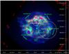 |
Fig. 1 Multi-colour image (Dec vs. RA in J2000) of Cas A produced using Chandra X-ray data. The red, green, and blue colour hues represent the energy ranges of [0.7, 1.0], [1.0, 3.5], and [3.5, 8.0] keV, respectively. The red and green hues are smoothed in linear colour scale, while the blue hues are shown in logarithmic scale to enhance the view of the smallest number of X-ray counts existing in the outer shell. The green ellipses represent the S, SW, SE, NW, and NE of the shell. The green and yellow crosses and dashed circles correspond to the VERITAS and MAGIC locations and approximated location error circles. The white cross and dashed circle are for the GeV gamma-ray emission best-fit location and the location error circle from the analysis in this paper. The CCO location is shown with a cyan open diamond. The red contours represent the derived CO data from Spitzer-IRAC starting from a value of 0.4 MJy/sr and higher. |
Figure 1 shows the Chandra X-ray image of Cas A, where the blue tones are the highest energy counts (3.5−8 keV), while red and green tones are the lower energy ranges of 0.7−1.0 and 1.0−3.5 keV, respectively. The selected regions contain filaments dominated by non-thermal emission (Yamazaki et al. 2004; Bamba et al. 2005; Araya et al. 2010; Araya & Frutos 2012), which mostly shine in X-ray energies between 3.5 and 8 keV. The locations (with green, yellow, and white crosses) and location errors (with green, yellow, and white dashed circles) of the TeV and GeV gamma-ray emissions, as measured by VERITAS, MAGIC, and Fermi-LAT, respectively, are also shown in Fig. 1. The CO data derived from Spitzer-IRAC with a starting value of 0.4 MJy/sr and higher is represented by red contours. The TeV locations found by VERITAS and MAGIC are more towards the east and south-east of the shell, while the GeV location of Fermi-LAT is towards the inner northern part of the remnant. However, the point-spread function of a point-like source of all three detectors is bigger in comparison to the radio size of the shell (5′). Therefore, it is not certain in which part of the shell the GeV and TeV gamma-ray emissions dominate.
The X-ray spectrum of each selected filament region was first fit with a xspec powerlaw by adding a wabs additive model that corresponds to photoelectric absorption of hydrogen. Then the spectra were fit to emission lines of iron, silicon, sulphur using Gaussian components. For each region, we obtained the following fit parameters: spectral index and flux normalisation. These two parameters are used for calculating the flux of each region. The X-ray fluxes of the S, SE, SW, NE, and NW regions are shown in Fig. 2 with data points in green, blue, magenta, cyan, and brown, respectively. The corresponding best-fit observed spectra are shown by black lines. We also analysed the whole remnant in a similar way as that for the selected filament regions. The observed X-ray spectrum that corresponds to the whole remnant is represented by the red data points and the best-fit spectrum by black line in Fig. 2.
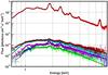 |
Fig. 2 X-ray spectra of the five different shell regions and the whole remnant: (a) green for S, (b) blue for SE, (c) magenta for SW, (d) cyan for NE, (e) brown for NW, and (f) red for the whole remnant. Corresponding best-fit X-ray spectra are shown by black lines. |
2.2. Gamma-rays
We analysed the GeV gamma-ray data of Fermi-LAT using the standard Fermi science tools (FST) package1 and the alternative package called pointlike (Kerr 2011; Lande et al. 2012), which is based on gtlike (FST-v9r27p1). The results of the analysis performed using the standard FST were published in Bozkurt et al. (2013). For the pointlike analysis, the data used was from 2008-08-04 to 2013-06-26 (~60 months) for energies between 200 MeV and 300 GeV. The gamma-ray events were selected from a circular region with a radius of 12° centred at RA(J2000) =  and Dec(J2000) =
  . Using gtselect of FST, the event-type was selected to do galactic point source analysis with Fermi-LAT Pass 7. To prevent event confusion caused by the bright gamma-rays from the Earth’s limb, we eliminate the gamma-rays having reconstructed zenith angles bigger than 105°. The radius of the analysis region (ROI) was chosen as 2.̊0.
The gamma-ray events in the data were binned in logarithmic energy steps between 200 MeV and 300 GeV. The spectral properties of the gamma-ray emission were studied by comparing the observation with models of possible sources in the ROI. Predictions were made by convolving the spatial distribution and spectrum of the source models with the instrument response function (IRF) and with the exposure of the observation. In the analysis, we used the IRF version P7SOURCE_V6.
The model of the analysis region contains the diffuse background sources and all point-like sources from the 2nd Fermi-LAT catalog that is located at a distance equal to or smaller than 1.̊8 away from the centre of the ROI. The standard background model has two components: diffuse galactic emission (gal_2yearp7v6_v0.fits) and an isotropic component (iso_p7v6source.txt). The background and source modelling was done using the gtlike, and the best set of spectral parameters of the fit were calculated by varying the parameters until the maximum likelihood was maximized.
The detection of the source is given approximately as the square root of the test statistics (TS), where larger TS values indicate that the maximum likelihood value for a model without an additional source (the null hypothesis) is incorrect. Cas A was detected with a significance of ~37σ at the best-fit location of RA = 350.̊87 ± 0.̊01 and Dec = 58.̊83 ± 0.̊01. The spectrum of Cas A was modelled by a power-law function, resulting in a spectral index value of Γ = 2.03 ± 0.02stat and a total photon flux of Fp = (6.17 ± 0.08stat) × 10-8 photons cm-2 s-1. The energy flux was found as Fe = (7.21 ± 0.05stat) × 10-11 erg cm-2 s-1 in the energy interval of 0.2−300 GeV. The spectral data points of the GeV emission are shown as blue triangles in Fig. 4. In addition, we have modelled the spectrum with a broken-power-law function, and we obtained the spectral indices to be Γ1 = 1.80 ± 0.05stat, Γ2 = 2.41 ± 0.06stat, and the break energy at Eb = 4.31 ± 0.37stat GeV. The total photon and energy fluxes were found to be Fp = (4.33 ± 0.14stat) × 10-8 photons cm-2 s-1 and Fe = (5.60 ± 0.07stat) × 10-11 erg cm-2 s-1, respectively. These results agree with the Fermi-LAT results found by Yuan et al. (2013) and Abdo et al. (2010).
3. Modelling the spectrum
3.1. Leptonic model
The non-thermal X-ray emission in the selected regions (i.e., S, SE, SW, NE, and NW) can be explained by the synchrotron emission from relativistic electrons in the source. Since relativistic particle spectra fall off roughly exponentially based on either an acceleration time scale (Drury 1991) or radiative loss (Webb et al. 1984), we consider a relativistic electron distribution that follows a powerlaw with an exponential cut-off, as shown in Eq. (1): 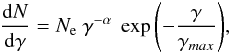 (1)where Ne and γmax are the constant of proportionality of electron distribution and the Lorentz factor of the cut-off energy of the electrons, respectively. The spectrum of the synchrotron radiation for a power-law distributed electrons can be written as (Blumenthal & Gould 1970),
 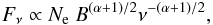 (2)where B is the magnetic field in the emission volume. Equation (2) shows that the synchrotron radiation depends on three parameters, Ne, B, and α. From the observed radio spectrum, Sν ∝ ν-0.77 (Baars et al. 1977), the power-law spectral index, α, is estimated to be 2.54. Hence, the value of Fν now changes with Ne (which is a measure of the electron density in the SNR) and magnetic field (B). Atoyan et al. (2000) developed a two-zone model, where the magnetic fields from the radio knots (zone one) and from the shell of the remnant (zone two) were estimated based on the observed radio data. In this two-zone scenario of Cas A, the magnetic field energy densities are different for two different zones, but the density of relativistic electrons in these zones are comparable to each other. Hence, we used the uniform electron density for all the shell regions in our model calculations. If Ne is fixed, then the level of synchrotron flux depends only on the magnetic field.
The Chandra observations from different regions of the shell show unequal levels of X-ray fluxes, which are attributed to different magnetic fields in those regions. These different magnetic fields thus contribute to the gamma-ray fluxes through inverse Compton (IC) and bremsstrahlung processes. To estimate the contribution to gamma-rays, we first considered that the whole remnant is uniform in X-ray flux and the southern part of the remnant contains only a fraction of the flux from the whole remnant. In the two-zone model of Cas A (Atoyan et al. 2000), the mean magnetic field in the shell region was found to be 300 μG, and the energy content of relativistic electrons in this region was calculated to be about 1048 erg. Here, we assumed a somewhat lower magnetic field, that is, 250 μG for the S-region of the shell and the other model parameters for the synchrotron emission process were estimated from the fit to the corresponding observed best-fit X-ray data. Afterwards, we estimated the magnetic fields for all other regions using the same electron density and same power-law spectral index. The calculated magnetic field values for all the shell regions are shown in Table 1. Based on the flux upper limit given by SAS-2 and COS B detectors, a lower limit on the magnetic field in the shell of Cas A was estimated to be 80 μG (Cowsik & Sarkar 1980), and our estimated magnetic fields do not violate this lower limit on the magnetic field. The rest of the parameters are fixed for all the regions, which are the following: spectral index, α = 2.54, γmax = 3.2 × 10⁷, and distance = 3.4 kpc. The fitted synchrotron spectra and the observed best-fit X-ray spectra for different regions are shown by lines and stripes, respectively, in Fig. 3.
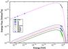 |
Fig. 3 Synchrotron spectra with the observed best-fit X-ray data for different regions of the shell. The spectral index describing radio-emitting electrons for all the regions is α = 2.54. The estimated magnetic fields for different shell regions are: 250 μG for S (solid line); 330 μG for SE (dashed line) and SW (dotted line); 410 μG for NE (dot-dashed line); 510 μG for NW (long-dash-dotted line), and 250 μG for the whole remnant (double-dot-dashed line). The best-fit X-ray fluxes of the S, SE, SW, NE, NW, and the whole remnant are shown with green, blue, magenta, cyan, brown, and black stripes. |
Magnetic field parameters for the synchrotron spectra for all selected regions.
The inverse Compton (IC) emission spectrum for the whole remnant was estimated using the parameters of the leptonic model obtained for each of the regions in the shell. The IC spectrum can be estimated in two different ways for each of the regions in the shell. First, the magnetic field for each region was considered to be the mean magnetic field for the whole remnant. Then parameters for the input spectrum were obtained from the fit to the observed radio and X-ray data. Once all the parameters for leptonic model were estimated, IC spectrum could be calculated. Secondly, we multiplied the radio synchrotron spectrum for each region with a scale factor, which was estimated by dividing the whole remnant’s observed radio or X-ray flux by the corresponding estimated synchrotron flux of this shell region. By considering scattering of electrons on far infra-red dust emission at T = 97 K, which dominates over cosmic microwave background photons as seed photons in the emission process (Atoyan et al. 2000), the IC spectra are shown in Fig. 4 for the shell regions. If the shell region is dominated by strong magnetic field (e.g. 510 μG), then the IC component of radiation is reduced, which is evident from Fig. 4. It shows that the TeV flux from the S-region of the shell is higher than those from other regions of Cas A.
It is evident from Fig. 4 that the TeV data at higher energy bins fit better with the IC prediction for the S-region among all other regions. However, the Fermi-LAT spectral data points at GeV energies cannot be explained by the IC mechanism alone, and it has to be modelled by an additional component, like the bremsstrahlung process or the neutral pion decay model.
Therefore, we estimated the contribution of bremsstrahlung process to explain fluxes at both GeV and TeV energies. The parameters corresponding to the S-region was used to calculate the bremsstrahlung spectrum considering ambient proton density to be nH = 10 cm-3 (Laming & Hwang 2003). The total energy of the electrons was estimated to be We = 4.8 × 1048 erg. The parameters used for this emission process is shown in Table 2. Figure 5 shows that the bremsstrahlung process alone cannot explain the GeV and TeV data simultaneously. Since the bremsstrahlung flux depends linearly on the ambient proton density, higher values of ambient proton density can increase the GeV−TeV fluxes to observed fluxes at these energies. Using the mass of supernova ejecta, Mejecta = 2 M⊙ (Willingale et al. 2003; Laming & Hwang 2003), where M⊙ is the solar mass, the effective gas density was found to be neff ≃ 32 cm-3 (Abdo et al. 2010). It is also not possible to explain GeV−TeV data with this density of ambient gas. Moreover, Fig. 5 shows that the shape of the observed GeV spectrum near 1 GeV is different from that of bremsstrahlung spectrum, which rises as it goes from GeV to lower energies.
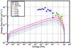 |
Fig. 4 IC spectra of the whole remnant, based on parameters related to different parts of the shell. The spectra for those regions are shown by the following lines: S by solid line, SE region by dotted line, SW by dashed line, NE by dot-dashed line, and NW by long-dashed-dotted line. The spectra for SE and SW are overlapping. The parameters for radio emitting electrons are α = 2.54, γmax = 3.2 × 10⁷. |
Parameters for bremsstrahlung process for the S-region of the SNR.
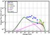 |
Fig. 5 Gamma-ray spectrum for Cas A. The IC (solid line) and bremsstrahlung (dashed line) spectra are estimated for the whole remnant when parameters are based on S-region of the shell. Bremsstrahlung spectrum is calculated for nH = 10 cm-3. The thick solid line corresponds to total contribution to gamma-rays from leptons. The parameters for radio-emitting electrons are α = 2.54,γmax = 3.2 × 10⁷. |
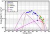 |
Fig. 6 Same as Fig. 5. Only π0 decay spectrum for the power-law distributed proton spectra (long-dash-dotted line) is included. The parameters used to get the π0 decay spectrum are shown in Table 3 by parameter Set-I. The estimated total energy of the protons, Wp = 5.7 × 1049 erg. |
3.2. Hadronic model
Since the leptonic model is not able to account for the observed gamma-ray emission at GeV energies, we need to invoke hadronic scenario to explain observed GeV fluxes. The gamma-ray flux resulting from the neutral pion (π0) decay of accelerated protons was estimated by considering ambient proton density to be 10 cm-3. The accelerated protons were considered to follow a broken power-law spectrum with an exponential cut-off as shown in Eq. (3). 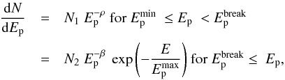 (3)where N1 and N2 are two normalisation constants and α and β are spectral indices before and after the break at
  . Figure 6 shows the contribution of gamma-ray flux from the π0 decay calculated following Kelner et al. (2006). The gamma-ray spectrum was fitted within the observed GeV−TeV energy range (see Fig. 6), and the corresponding best fit parameters are shown in Set-I of Table 3. The total energy of the protons in the hadronic model was estimated to be Wp = 5.7 × 1049(10 cm-3/nH) erg. We would like to note that we are considering gamma-ray spectrum for the whole remnant, because the angular resolution for the current generation gamma-ray instruments are not comparable to the X-ray instruments.
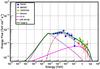 |
Fig. 7 Gamma-ray spectrum (thick solid line) for Cas A for combining both leptonic and hadronic contribution to the whole remnant data. Parameters for leptonic model spectra (IC: solid line and bremsstrahlung: dashed line) correspond to S-region of the remnant. Parameters for hadronic model are shown in Table 3 by Set-II (long-dash-dotted line). |
Parameters for gamma-ray production through decay of neutral pions.
It has been already mentioned in Sect. 3.1 that the leptonic model can only account for the TeV fluxes at the highest energy bins, whereas the observed GeV fluxes can be explained by hadronic model as shown in Fig. 6. To get a complete understanding of the spectrum at GeV−TeV energies, we have to estimate the combined spectrum resulting from both leptonic and hadronic model (hereafter, lepto-hadronic model). Since the parameters for the leptonic model are fixed by observed radio and X-ray fluxes, the resulting parameters for the hadronic model for the combined GeV−TeV spectrum are different from the parameters listed in Table 3 (see Set-I). The best-fit parameters for the lepto-hadronic model are given in Set-II of Table 3, and it shows that the corresponding χ2 value is less than that of purely hadronic model. The corresponding spectrum is shown in Fig. 7. The maximum energy of protons ( ) is fixed to 100 TeV for both pure hadronic and lepto-hadronic model. The total energy of the charged particles for the lepto-hadronic model is We + Wp = 3.4 × 1049 erg, which gives a conversion efficiency of supernova explosion energy to be less than 2%, which is consistent with that value calculated by Yuan et al. (2013). Although the GeV data corresponds to the best fit location as shown in Fig. 1 using white dashed circle, it is to be mentioned that the gamma-rays are not being emitted from other regions of Cas A. Hence, there is no harm in combing GeV−TeV data to get best fitted emission model.
4. Discussion
The aim of this paper is to locate the region of the shell of Cas A, which is brightest in gamma-rays and to interpret the observed fluxes at GeV−TeV energies in the context of both leptonic and hadronic models. From the different levels of X-ray flux in several shell regions, we found that the magnetic fields are different in those regions. Since IC flux becomes less significant with higher magnetic field, the NW region of the shell of the remnant is less significant in producing gamma-ray fluxes through IC process among all other shell regions. On the other hand, the S-region of the remnant becomes a significant region for production of IC fluxes due to the lower magnetic field in this region. Although we have considered same spectral index for radio emitting electrons, different choices of spectral indices do not change the overall conclusion.
In addition, we see from Fig. 5 that IC fluxes can explain the data only at TeV energies while the bremsstrahlung process is unable to explain the GeV−TeV data for ambient gas density 10 cm-3. Moreover, the bremsstrahlung process was also unable to explain the observed fluxes properly with higher values of ambient gas density (~32 cm-3). Therefore, we conclude that the leptonic scenario is insufficient to explain the observed GeV and TeV gamma-ray fluxes simultaneously. Hence, we need to invoke hadronic contribution to account for the observed gamma-ray fluxes. The gamma-ray spectrum that results from decay of π0s in Fig. 6 shows that it alone can explain the GeV and TeV fluxes with a χ2 value of 2.5. Since we have already seen that the leptonic scenario can contribute to TeV energies, we cannot ignore this completely. So we estimated the total contribution from both the leptonic and hadronic model to explain the data. Figure 7 shows that the gamma-ray spectrum due to decay of π0 along with leptonic model is able to explain the GeV−TeV gamma-rays for the ambient gas density of 10 cm-3. Moreover, the best fit χ2 value for this case is less than that of the case of purely hadronic model, as shown in Table 3. Although increasing the effective density of the ambient gas to higher values (than the estimated average density) may help the bremsstrahlung model to reach the level of GeV−TeV data, the gamma-ray fluxes due to the π0 decay of accelerated protons also increase. Therefore, the π0 decay process is no longer be able explain the GeV−TeV data unless the total energy budget of the protons is reduced. That, in turn, indicates a lower conversion efficiency of the explosion energy of Cas A into accelerating protons. The GeV flux that falls below 1 GeV is considered to be a clear indication for the π0 decay origin of gamma-ray emission. Very recently, Yuan et al. (2013) reported that their Fermi-LAT data analysis of Cas A resulted in the gamma-ray emission to be hadronic in nature. A higher density of ambient gas may establish the fact of having higher potential for producing gamma-rays through π0 −decay process for the S-region. Nevertheless, the total contribution to TeV energies due to both leptonic and hadronic models cannot be ignored.
According to Vink & Laming (2003), the magnetic field at the forward shock is within the range of 80−160 μG, whereas the mean magnetic field value in the shell of Cas A was estimated to be ~300 μG by Atoyan et al. (2000) and Parizot et al. (2006). Although Abdo et al. (2010) showed that the leptonic model for the magnetic field of 120 μG can broadly explain the observed GeV−TeV fluxes, the corresponding spectrum from leptonic model does not fit well. With a lower value of the magnetic field (i.e. <120 μG), the TeV fluxes can be overestimated by IC emission spectrum. If we consider the magnetic field for the S-region of the shell to be about 120 μG, the lepto-hadronic model has to be sufficiently modified to explain the total fluxes. The total fluxes from the lepto-hadronic model exceeds the observed values, and the corresponding χ2 value for the best fit parameters becomes large. This overestimated flux cannot be compensated by lowering the contribution from hadronic model. Hence, we need to consider higher values of magnetic field (~250 μG), so that the total spectrum from lepto-hadronic model can explain the data sufficiently better than both a pure leptonic and a pure hadronic model.
The most interesting result is the relatively low total accelerated particle energy (of the order of 2% conversion efficiency) that is combined with the high magnetic field estimate. This amplification of a magnetic field can either be related through magneto-hydrodynamic waves generated by cosmic rays (Bell & Lucek 2001; Bell 2004) or could result from the effect of turbulent density fluctuations on the propagating hydrodynamic shock waves, which has been observed through two-dimensional magneto-hydrodynamic numerical simulations (Giacalone & Jokipii 2007). The low conversion efficiency of cosmic rays suggests that the cosmic ray streaming energy may not be sufficient enough to be transferred to the magnetic fields that result from magnetic amplification. Hence, the magnetic field amplification in the down-stream of shocks due to presence of turbulence could be favourable in this particular remnant.
It is to be mentioned that the differences in the X-ray flux levels for different regions of Cas A can be attributed to the different densities of the injection of the electrons. For different densities, however, there may not be any difference in gamma-ray fluxes from different regions of the shell. However, this needs a detailed investigation of the density profile of the relativistic electrons in this source.
5. Conclusion
We found that the gamma-ray emission from the S-region of the shell through IC process has the highest flux value, and this predicted flux matches better to the TeV data in comparison to flux predictions from other regions of the shell. The second best-fit IC prediction with the TeV data is from the SE and SW and then the NE region. We also found that the leptonic model alone is unable to explain observed GeV fluxes for any regions of the shell. However, the GeV and TeV gamma-ray data fits reasonably well to the hadronic model, which is independent of the selected regions on the shell.
If the SNR would be perfectly symmetric in shape, we would expect that the fluxes of each region of the shell should be equal. Apparently, the shell’s emission is not homogeneously distributed. The reason for the variations in X-ray and gamma-ray fluxes can be due to different amounts of particles or variations in the magnetic field at different regions of the SNR’s shell. The molecular environment might also be different at different sides of the shell. Future gamma-ray instruments with far better angular resolution (e.g., CTA) will be required to understand the spectral and spatial structure of the remnant in gamma-rays.
Acknowledgments
We would like to thank Prof. Jeonghee Rho for providing us CO data from Spitzer-IRAC. T.E. acknowledges support from the Scientific and Technological Research Council of Turkey (TÜBİTAK) through the BİDEB-2232 fellowship program. This work was supported by Boğaziçi University. E.N.E. thanks to Bog˜aziçi University BAP support through a project of code 5052P. We would also like to thank the referee of this paper for his comments and suggestions.
References
- Abdo, A. A., Ackermann, M., Ajello, M., et al. 2010, ApJ, 710, L92 [NASA ADS] [CrossRef] [Google Scholar]
- Acciari, V. A., Aliu, E., Arlen, T., et al. 2010, ApJ, 714, 163 [Google Scholar]
- Aharonian, F., Akhperjanian, A., Barrio, J., et al. 2001, A&A, 370, 112 [NASA ADS] [CrossRef] [EDP Sciences] [Google Scholar]
- Albert, J., Aliu, E., Anderhub, H., et al. 2007, A&A, 474, 937 [NASA ADS] [CrossRef] [EDP Sciences] [Google Scholar]
- Allen, G. E., Keohane, J. W., & Gotthelf, E. V. 1997, ApJ, 487, L97 [NASA ADS] [CrossRef] [Google Scholar]
- Anderson, M. C., Keohane, J. W., & Rudnick, L. 1995, ApJ, 441, 300 [NASA ADS] [CrossRef] [Google Scholar]
- Araya, M., & Cui, W. 2010, ApJ, 720, 20 [NASA ADS] [CrossRef] [Google Scholar]
- Araya, M., & Frutos, F. 2012, MNRAS, 425, 2810 [NASA ADS] [CrossRef] [Google Scholar]
- Araya, M., Lomiashvili, D., Chang, C., Lyutikov, M., & Cui, W. 2010, ApJ, 714, 396 [NASA ADS] [CrossRef] [Google Scholar]
- Atoyan, A. M., Tuffs, R. J., Aharonian, F. A., & Völk, H. J. 2000, A&A, 354, 915 [NASA ADS] [Google Scholar]
- Baars, J. W. M., Genzel, R., Pauliny-Toth, I. I. K., & Witzel, A. 1977, A&A, 61, 99 [NASA ADS] [Google Scholar]
- Bamba, A., Yamazaki, R., Yoshida, T., Terasawa, T., & Koyama, K. 2005, ApJ, 621, 793 [NASA ADS] [CrossRef] [Google Scholar]
- Bell, A. R. 2004, MNRAS, 353, 550 [Google Scholar]
- Bell, A. R., & Lucek, S. G. 2001, MNRAS, 321, 433 [NASA ADS] [CrossRef] [Google Scholar]
- Blumenthal, G. R., & Gould, R. J. 1970, Rev. Mod. Phys., 42, 237 [NASA ADS] [CrossRef] [Google Scholar]
- Bozkurt, M., Ergin, T., Hudaverdi, M., & Ercan, E. N. 2013, Int. J. Astron. Astrophys., 3, 34 [CrossRef] [Google Scholar]
- Cowsik, R., & Sarkar, S. 1980, MNRAS, 191, 855 [NASA ADS] [Google Scholar]
- Delaney, T., Rudnick, L., Stage, M. D., et al. 2010, ApJ, 725, 2038 [NASA ADS] [CrossRef] [Google Scholar]
- Drury, L. O’C. 1991, MNRAS, 251, 340 [NASA ADS] [Google Scholar]
- Ergin, T., Saha, L., Majumdar, P., Bozkurt, M., & Ercan, E. N. 2013, Proc. ICRC 2013 [arXiv:1308.0195] [Google Scholar]
- Esposito, J. A., Hunter, S. D., Kanbach, G., & Sreekumar, P. 1996, ApJ, 461, 820 [NASA ADS] [CrossRef] [Google Scholar]
- Giacalone, J., & Jokipii, J. R. 2007, ApJ, 663, L41 [NASA ADS] [CrossRef] [Google Scholar]
- Gotthelf, E. V., Koralesky, B., Rudnick, L., et al. 2001, ApJ, 552, L39 [NASA ADS] [CrossRef] [Google Scholar]
- Helder, E. A., & Vink, J. 2008, ApJ, 686, 1094 [NASA ADS] [CrossRef] [Google Scholar]
- Helmboldt, J. F., & Kassim, N. E. 2009, AJ, 138, 838 [NASA ADS] [CrossRef] [Google Scholar]
- Hughes, J. P., Rakowski, C. E., Burrows, D. N., & Slane, P. O. 2000, ApJ, 528, L109 [NASA ADS] [CrossRef] [PubMed] [Google Scholar]
- Hwang, U., Laming, J. M., Badenes, C., et al. 2004, ApJ, 615, 117 [Google Scholar]
- Kelner, S. R., Aharonian, F. A., & Bugayov, V. V. 2006, Phys. Rev. D, 74, 034018 [NASA ADS] [CrossRef] [Google Scholar]
- Kerr, M. 2011 [arXiv:1101.6072] [Google Scholar]
- Laming, J. M., & Hwang, U. 2003, ApJ, 597, 347 [NASA ADS] [CrossRef] [Google Scholar]
- Lande, J., Ackermann, M., Allafort, A., et al. 2012, ApJ, 756, 5 [Google Scholar]
- Maeda, Y., Uchiyama, Y., Bamba, A., et al. 2009, PASJ, 61, 1217 [NASA ADS] [CrossRef] [Google Scholar]
- Parizot, E., Marcowith, A., Ballet, J., & Gallant, Y. A. 2006, A&A, 453, 387 [NASA ADS] [CrossRef] [EDP Sciences] [Google Scholar]
- Patnaude, D. J., & Fesen, R. A. 2009, ApJ, 697, 535 [NASA ADS] [CrossRef] [Google Scholar]
- Pavlov, G. G., Zavlin, V. E., Aschenbach, B., Trümper, J., & Sanwal, D. 2000, ApJ, 531, L53 [NASA ADS] [CrossRef] [Google Scholar]
- Pavlov, G. G., Sanwal, D., & Teter, M. A. 2004, IAU Symp., 218, 239 [Google Scholar]
- Reed, J. E., Hester, J. J., Fabian, A. C., & Winkler, P. F. 1995, ApJ, 440, 706 [NASA ADS] [CrossRef] [Google Scholar]
- Rho, J., Jarrett, T. H., Reach, W. T., Gomez, H., & Andersen, M. 2009, ApJ, 693, L39 [NASA ADS] [CrossRef] [Google Scholar]
- Rho, J., Onaka, T., Cami, J., & Reach, W. T. 2012, ApJ, 747, L6 [NASA ADS] [CrossRef] [Google Scholar]
- Smith, J. D. T., Rudnick, L., Delaney, T., et al. 2009, ApJ, 693, 713 [NASA ADS] [CrossRef] [Google Scholar]
- Uchiyama, Y., & Aharonian, F. A. 2008, ApJ, 677, L105 [NASA ADS] [CrossRef] [Google Scholar]
- Vink, J., & Laming, J. M. 2003, ApJ, 584, 758 [NASA ADS] [CrossRef] [Google Scholar]
- Vinyaikin, E. N. 2007, Astron. Rev., 51, 87 [NASA ADS] [CrossRef] [Google Scholar]
- Yamazaki, R., Yoshida, T., Terasawa, T., Bamba, A., & Koyama, K. 2004, A&A, 416, 595 [NASA ADS] [CrossRef] [EDP Sciences] [Google Scholar]
- Wallstrom, S. H. J., et al. 2013, A&A, 558, L2 [NASA ADS] [CrossRef] [EDP Sciences] [Google Scholar]
- Webb, G. M., Drury, L. O’C., & Biermann, P. L. 1984, A&A, 137, 185 [NASA ADS] [Google Scholar]
- Willingale, R., Bleeker, J. A. M., van der Heyden, K. J., & Kaastra, J. S. 2003, A&A, 398, 1021 [NASA ADS] [CrossRef] [EDP Sciences] [Google Scholar]
- Yuan, Y., Funk, S., Jóhannesson, G., et al. 2013, ApJ, 779, 117 [NASA ADS] [CrossRef] [Google Scholar]
- Zirakashvili, V. N., & Aharonian, F. A. 2010, ApJ, 708, 965 [NASA ADS] [CrossRef] [Google Scholar]
All Tables
All Figures
|
Fig. 1 Multi-colour image (Dec vs. RA in J2000) of Cas A produced using Chandra X-ray data. The red, green, and blue colour hues represent the energy ranges of [0.7, 1.0], [1.0, 3.5], and [3.5, 8.0] keV, respectively. The red and green hues are smoothed in linear colour scale, while the blue hues are shown in logarithmic scale to enhance the view of the smallest number of X-ray counts existing in the outer shell. The green ellipses represent the S, SW, SE, NW, and NE of the shell. The green and yellow crosses and dashed circles correspond to the VERITAS and MAGIC locations and approximated location error circles. The white cross and dashed circle are for the GeV gamma-ray emission best-fit location and the location error circle from the analysis in this paper. The CCO location is shown with a cyan open diamond. The red contours represent the derived CO data from Spitzer-IRAC starting from a value of 0.4 MJy/sr and higher. |
| In the text | |
|
Fig. 2 X-ray spectra of the five different shell regions and the whole remnant: (a) green for S, (b) blue for SE, (c) magenta for SW, (d) cyan for NE, (e) brown for NW, and (f) red for the whole remnant. Corresponding best-fit X-ray spectra are shown by black lines. |
| In the text | |
|
Fig. 3 Synchrotron spectra with the observed best-fit X-ray data for different regions of the shell. The spectral index describing radio-emitting electrons for all the regions is α = 2.54. The estimated magnetic fields for different shell regions are: 250 μG for S (solid line); 330 μG for SE (dashed line) and SW (dotted line); 410 μG for NE (dot-dashed line); 510 μG for NW (long-dash-dotted line), and 250 μG for the whole remnant (double-dot-dashed line). The best-fit X-ray fluxes of the S, SE, SW, NE, NW, and the whole remnant are shown with green, blue, magenta, cyan, brown, and black stripes. |
| In the text | |
|
Fig. 4 IC spectra of the whole remnant, based on parameters related to different parts of the shell. The spectra for those regions are shown by the following lines: S by solid line, SE region by dotted line, SW by dashed line, NE by dot-dashed line, and NW by long-dashed-dotted line. The spectra for SE and SW are overlapping. The parameters for radio emitting electrons are α = 2.54, γmax = 3.2 × 10⁷. |
| In the text | |
|
Fig. 5 Gamma-ray spectrum for Cas A. The IC (solid line) and bremsstrahlung (dashed line) spectra are estimated for the whole remnant when parameters are based on S-region of the shell. Bremsstrahlung spectrum is calculated for nH = 10 cm-3. The thick solid line corresponds to total contribution to gamma-rays from leptons. The parameters for radio-emitting electrons are α = 2.54,γmax = 3.2 × 10⁷. |
| In the text | |
|
Fig. 6 Same as Fig. 5. Only π0 decay spectrum for the power-law distributed proton spectra (long-dash-dotted line) is included. The parameters used to get the π0 decay spectrum are shown in Table 3 by parameter Set-I. The estimated total energy of the protons, Wp = 5.7 × 1049 erg. |
| In the text | |
|
Fig. 7 Gamma-ray spectrum (thick solid line) for Cas A for combining both leptonic and hadronic contribution to the whole remnant data. Parameters for leptonic model spectra (IC: solid line and bremsstrahlung: dashed line) correspond to S-region of the remnant. Parameters for hadronic model are shown in Table 3 by Set-II (long-dash-dotted line). |
| In the text | |
Current usage metrics show cumulative count of Article Views (full-text article views including HTML views, PDF and ePub downloads, according to the available data) and Abstracts Views on Vision4Press platform.
Data correspond to usage on the plateform after 2015. The current usage metrics is available 48-96 hours after online publication and is updated daily on week days.
Initial download of the metrics may take a while.