| Issue |
A&A
Volume 563, March 2014
|
|
|---|---|---|
| Article Number | A18 | |
| Number of page(s) | 9 | |
| Section | The Sun | |
| DOI | https://doi.org/10.1051/0004-6361/201322635 | |
| Published online | 27 February 2014 | |
A solar dynamo model driven by mean-field alpha and Babcock-Leighton sources: fluctuations, grand-minima-maxima, and hemispheric asymmetry in sunspot cycles
1 CENTRA, Instituto Superior Técnico, Universidade de Lisboa, Av. Rovisco Pais, 1049-001 Lisboa, Portugal
e-mail: This email address is being protected from spambots. You need JavaScript enabled to view it.
2 Departamento de Física, Universidade de Évora, Colégio António Luis Verney, 7002-554 Évora, Portugal
3 GRPS, Départment de Physique, Université de Montréal, CP 6128, Centre-ville, Montréal, Qc, H3C-3J7, Canada
4 Department of Physical Science, Indian Institute of Science Education and Research, Kolkata, 741252 Mohanpur, West Bengal, India
5 Center of Excellence in Space Sciences India, Indian Institute of Science Education and Research, Kolkata, 741252 Mohanpur, West Bengal, India
e-mail: This email address is being protected from spambots. You need JavaScript enabled to view it.
Received: 9 September 2013
Accepted: 31 December 2013
Abstract
Context. Extreme solar activity fluctuations and the occurrence of solar grand minima and maxima episodes, such as the Maunder minimum and Medieval maximum are well-established, observed features of the solar cycle. Nevertheless, such extreme activity fluctuations and the dynamics of the solar cycle during Maunder minima-like episodes remain ill understood.
Aims. We explore the origin of such extreme solar activity fluctuations and the role of dual poloidal field sources, namely the Babcock-Leighton mechanism and the mean-field α effect in the dynamics of the solar cycle. We mainly concentrate on entry and recovery from grand minima episodes such as the Maunder minimum and the dynamics of the solar cycle, including the structure of solar butterfly diagrams during grand minima episodes.
Methods. We use a kinematic solar dynamo model with a novel set-up in which stochastic perturbations force two different poloidal sources. We explore different regimes of operation of these poloidal sources with distinct operating thresholds to identify the importance of each. The perturbations are implemented independently in both hemispheres which allows the study of the level of hemispheric coupling and hemispheric asymmetry in the emergence of sunspots.
Results. From the simulations performed we identify a few different ways in which the dynamo can enter a grand minima episode. While fluctuations in any of the α effects can trigger intermittency, in keeping with results from a mathematical time-delay model we find that the mean-field α effect is crucial for the recovery of the solar cycle from a grand minima episode, which a Babcock-Leighton source alone fails to achieve. Our simulations also demonstrate many types of hemispheric asymmetries, including grand minima and failed grand minima where only one hemisphere enters a quiescent state.
Conclusions. We conclude that stochastic fluctuations in two interacting poloidal field sources working with distinct operating thresholds is a viable candidate for triggering episodes of extreme solar activity and that the mean-field α effect capable of working on weak, sub-equipartition fields is critical to the recovery of the solar cycle following an extended solar minimum. Based on our results, we also postulate that solar activity can exhibit significant parity shifts and hemispheric asymmetry, including phases when only one hemisphere is completely quiescent while the other remains active, to, successful grand minima like conditions in both hemispheres.
Key words: Sun: activity / Sun: magnetic fields / Sun: evolution / sunspots / Sun: interior
© ESO, 2014
1. Introduction
For hundreds of years mankind has kept a close eye on the evolution of our star. Since the advent of the telescope, solar activity has been monitored systematically, creating one of the longest continuous observation programmes in the history of science (Owens 2013), the sunspot number measurements. These solar features continue to be used as the most common proxy for solar magnetic activity as their appearance on the Sun’s surface is thought to be connected with the build-up of large-scale, coherent magnetic fields in the solar convection zone (SCZ) mainly in the azimuthal direction, the so called toroidal magnetic field component. This field component is produced by a magnetohydrodynamic (MHD) dynamo that converts a portion of the kinetic energy of the solar differential rotation into magnetic energy (Parker 1955). This process takes place in a thin shear layer at the bottom of the SCZ, known as the tachocline, between the turbulent convection zone and the underlying stable overshoot layers. The most common theoretical framework used to explain the origin and evolution of the large-scale solar magnetic field is the mean-field dynamo theory (Steenbeck et al. 1966). Models based on this theory solve a simplified version of the MHD induction equation, usually in spherical-polar coordinates under some physically inspired simplifications such as axisymmetry and spatio-temporal averages of the magnetic field (see review by Charbonneau 2010). Considered by some as the most successful of these models, Babcock-Leighton (BL) flux transport dynamo models (Wang et al. 1991; Durney 1995; Dikpati & Charbonneau 1999; Nandy & Choudhuri 2002) have become very useful tools for explaining the main features of the solar cycle such as its periodicity, parity, the migration pattern of sunspots towards the equator and the phase difference between the toroidal and dipolar magnetic fields. These models incorporate the solar meridional circulation and emulate the effect of the decay of active regions for the production of the poloidal field based on the original ideas of Babcock and Leighton (Babcock & Babcock 1955; Leighton 1969).
For many decades, the importance of the BL surface mechanism was overshadowed by another type of poloidal field source, the mean-field α effect (or Parker’s α effect) in mean-field αΩ dynamos. In this type of dynamo model, the source for transforming a toroidal field into a poloidal field is the action of helical turbulence in the twisting of flux tubes as they buoyantly rise through the SCZ (Charbonneau 2010). The mean-field α effect is thought to be quenched by super-equipartition magnetic fields and to be effective only on relatively weaker fields. Works such as D’Silva & Choudhuri (1993) have raised questions regarding the effectiveness of this type of alpha effect by asserting that Joys’ Law distribution (tilt angle dependence on latitude of bipolar sunspot pairs) requires very strong, super-equipartition toroidal field strengths; see also Fan (2001). Moreover, recent observational evidence points out that the BL mechanism is the predominant source for the solar cycle (Dasi-Espuig et al. 2010). Following these developments the stakes seem to be loaded against the mean-field α effect mechanism. Nevertheless, recent, realistic 3D MHD simulations of the SCZ (Käpylä et al. 2006; Brown et al. 2010; Racine et al. 2011), show clear evidence that a mean-field-type α effect should exist in the bulk of the convection zone. The question is whether this mean-field α plays a dynamically important role in the solar cycle.
Important constraints on dynamo models have emerged in the last decade based on long-term reconstructions of solar activity using cosmogenic isotopes (Miyahara et al. 2006; Usoskin et al. 2007; Usoskin 2008). These reconstructions show that in addition to the typical variability observed in the 11-year solar cycle, there are extended periods of time in which the Sun behaves in a very unusual way. Solar magnetic activity seems to exhibit intermittency (fluctuations and episodes of stronger than normal and quieter than normal activity), as it is usually defined in the jargon of Dynamic Systems. This means that there are periods where the normal cyclic activity ceases to exist and the Sun enters a grand minimum period. During these grand minima, the Sun exhibits a very low number (or lack) of sunspots in its photosphere and it is believed that the overall magnetic field also becomes very weak. Thanks to recent data, e.g. Steinhilber et al. (2012), we now know that these periods are much more common than previously thought and therefore they should be considered as a constraint on any model of the solar cycle. The most famous of these quiescent periods of activity is called the Maunder minimum that took place between 1645 and 1715 (Maunder 1904; Eddy 1976). This period of low solar activity coincided with a period of very low temperatures in the Earth’s northern hemisphere during the last part of the Little Ice Age. This and other interesting correlations between solar activity and the Earth’s climate have been found in the past (Haigh 2007). A vitally important aspect of the grand minima enigma is to understand how the solar dynamo reawakens from these quiescent phases and the dynamics leading to, during, and exiting the phases.
Over the years some authors have focussed their efforts in modelling and understanding the mechanisms behind the observed short- and long-term variability (e.g. amplitude variations from cycle to cycle and grand minima-maxima) of the solar cycle. Two major approaches are usually used in these studies, one that looks for dynamical effects and a second that studies the impact of stochasticity on the system. The dynamical mechanism approach is based on non-linear interactions between the magnetic field and plasma flows. One of the most important ingredients in any dynamo model is the differential rotation. So, it is only natural to assume that perturbations in this strong, large-scale flow can induce fluctuations in activity. The so called Malkus-Proctor effect, i.e. the feedback of the large-scale magnetic field on the rotation is such an example, wherein, strong magnetic fields quench the very flow which sustains dynamo action. This results in a weakening of magnetic activity, subsequently to which the Reynolds stresses restore the differential rotation to its initial state, thereby resuming activity (Tobias 1997; Brooke et al. 2002; Bushby 2006). While this remains a plausible scenario for activity modulation, recent analysis of global 3D MHD simulations of solar convection that present dynamo action, indicates that modulation effects on the differential rotation could be much smaller than previously thought (Beaudoin et al. 2012). Other examples of dynamical processes are the modulation of the meridional circulation by the magnetic field as seen in dynamo models working in the non-kinematic regime (Rempel 2006; Passos et al. 2012) and the time delay dynamics that are inherent in the dynamo system with spatially segregated source-layers (Charbonneau et al. 2005; Wilmot-Smith et al. 2006; Jouve et al. 2010).
The modelling approach based on stochastic fluctuations is motivated by the fact that the solar dynamo resides in a very turbulent environment, i.e. the SCZ. So it is highly plausible that some of the intervening physical mechanisms are affected by “noise” imparted by random processes that are the basis of turbulent convection. This is usually modelled as stochastic fluctuations around an average typical value of some model’s ingredient such as the α effect (Hoyng 1988; Choudhuri 1992; Hoyng 1993, 1994; Charbonneau et al. 2004; Usoskin 2008) or the meridional circulation (Charbonneau & Dikpati 2000; Lopes & Passos 2009; Karak 2010). Even if noise is introduced in the system at correlation timescales that are much shorter than the solar cycle timescale they tend to induce modulations on timescales ranging from decades to centennia. These models are also very robust because they can handle a wide range of noise levels. Some of these stochastically forced models have been very successful in providing a simple explanation for the observed short-term solar variability, and a few of them also display grand minima-like episodes as well. For the interested reader, a comprehensive review of modulation mechanisms of the solar dynamo can be found in Tobias (2002).
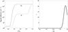 |
Fig. 1 Left panel: shows the toroidal (dashed) and poloidal (solid) magnetic diffusivity profiles. Right panel: radial profile of the α coefficient that is used to model the near-surface BL poloidal source (in m s-1). |
Here, we base our study on a stochastically forced, kinematic, BL dynamo model. Inspired by the study of Hazra et al. (2014, henceforth Paper I), we explore the role of stochastically forced, dual poloidal field sources in the context of grand minima and maxima in solar activity. In Paper I the authors present a novel solution to how the dynamo re-emerges from a grand minima episode. In that paper they used a time-delay low-order dynamo model to explore what happens when two α effects work simultaneously, one effective on weak toroidal fields (mean-field α) and another effective on stronger fields (BL α). They demonstrate that the weak mean-field effect has a crucial role in driving the dynamo out of a grand minimum and postulate the usage of both an upper and lower threshold for the BL α in order to avoid fake, i.e physically incorrect, recovery from grand minima episodes. Here we follow this postulate, test the original idea, and also study additional dynamics associated with extreme solar activity with a spatially extended solar dynamo model with solar-like differential rotation and other physically inspired parameterizations. We introduce a secondary, mean-field α effect in the bulk of the convection zone in our BL flux transport model and explore the consequent dynamics in the stochastically forced regime. Our results support the main conclusions presented in Paper I and we explore the subject further. In the following section we discuss the base model and show how fluctuations in the surface BL α effect induce the dynamo to enter a grand minima-like state. In the subsequent section we add the secondary mean-field α effect to the model, discuss the modifications introduced to the parametrization of both α effects, and demonstrate scenarios wherein stochastic fluctuations trigger grand maxima and minima behaviour and self-consistent recovery from them. We also analyse the resultant butterfly diagrams and demonstrate that hemispheric coupling during quiescent phases can range from strong asymmetry to near simultaneous occurrence of quiescent phases in both the northern and southern solar hemispheres. We end with a concluding section discussing the implications of our results and putting them in a broader context.
2. The model
The axisymmetric dynamo Eqs. (1) and (2) are solved in the kinematic regime using a modified version of the Surya - code (Nandy & Choudhuri 2002; Chatterjee et al. 2004). This code solves the equations
![Mathematical equation: \begin{eqnarray} &&\frac{\partial A}{\partial t} + \frac{1}{s}(\vec{v}\cdot\nabla)(s A) = \eta_{\rm p} \left( \nabla^2 - \frac{1}{s^2}\right)A + \alpha B, \label{eq:1}\\ && \frac{\partial B}{\partial t} + \frac{1}{r}\left[\frac{\partial}{\partial r}(r v_r B) + \frac{\partial}{\partial \theta}(v_\theta B)\right] = \eta_{\rm t} \left( \nabla^2 - \frac{1}{s^2}\right)B \nonumber \\ && \phantom{\frac{\partial B}{\partial t} + \frac{1}{r}\left[\frac{\partial}{\partial r}(r v_r B) + \frac{\partial}{\partial \theta}(v_\theta B)\right] = }+\, s ((\nabla \times [A(r,\theta)\vec{e}_\phi])\cdot\nabla)\Omega \nonumber \\ && \phantom{\frac{\partial B}{\partial t} + \frac{1}{r}\left[\frac{\partial}{\partial r}(r v_r B) + \frac{\partial}{\partial \theta}(v_\theta B)\right] = }+\, \frac{1}{r}\frac{{\rm d}\eta_{\rm t}}{{\rm d}r}\frac{\partial}{\partial r}(rB), \label{eq:2} \end{eqnarray}](/articles/aa/full_html/2014/03/aa22635-13/aa22635-13-eq4.png) where s = rsin(θ), v is the meridional flow, Ω the differential rotation, and α is a surface source term that emulates the BL mechanism. This numerical model assumes different magnetic diffusivities for the poloidal and toroidal field components, ηp and ηt, respectively. The use of two distinct diffusivity profiles in the Surya code is inspired by the reasoning that strong magnetic fields will suppress turbulence. Hence it is expected that in the strong field regions where the toroidal field resides turbulent diffusivity will be much less effective, while in the weak field regions occupied by the poloidal component the turbulent diffusivity will be higher (closer to values predicted by mixing length theory). This is a relatively simple, although effective technique for numerically capturing this physics. The model also has a built-in buoyancy algorithm that searches for a toroidal field exceeding a certain threshold (105G by default) at the base of the SCZ (at r = 0.71 R⊙) at certain time intervals, removes half of it, and deposits this field at near-surface layers where the BL poloidal source is located. This is done to emulate the eruption of magnetic flux tubes. For most of our simulations, Eqs. (1) and (2) are solved in a 256 × 256 grid between Rb = 0.55 R⊙ < r < R⊙ and 0 < θ < π under appropriate boundary conditions.
where s = rsin(θ), v is the meridional flow, Ω the differential rotation, and α is a surface source term that emulates the BL mechanism. This numerical model assumes different magnetic diffusivities for the poloidal and toroidal field components, ηp and ηt, respectively. The use of two distinct diffusivity profiles in the Surya code is inspired by the reasoning that strong magnetic fields will suppress turbulence. Hence it is expected that in the strong field regions where the toroidal field resides turbulent diffusivity will be much less effective, while in the weak field regions occupied by the poloidal component the turbulent diffusivity will be higher (closer to values predicted by mixing length theory). This is a relatively simple, although effective technique for numerically capturing this physics. The model also has a built-in buoyancy algorithm that searches for a toroidal field exceeding a certain threshold (105G by default) at the base of the SCZ (at r = 0.71 R⊙) at certain time intervals, removes half of it, and deposits this field at near-surface layers where the BL poloidal source is located. This is done to emulate the eruption of magnetic flux tubes. For most of our simulations, Eqs. (1) and (2) are solved in a 256 × 256 grid between Rb = 0.55 R⊙ < r < R⊙ and 0 < θ < π under appropriate boundary conditions.
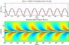 |
Fig. 2 Top panel: toroidal field amplitude, |

This code also uses a differential rotation profile, Ω(r,θ), that is an analytical fit to the solar internal rotation data provided by Helioseismology. The meridional circulation, v, has a one cell per hemisphere configuration, with latitudinal flows drifting towards the poles in the surface layers and towards the equator just below the tachocline. The amplitude of the surface component of this flow at mid latitudes is defined by v0 = −29 m s-1 (in the standard version of the code). Detailed description of mathematical parametrization of these quantities including their justifications, for this well tested dynamo code, are available elsewhere (Nandy & Choudhuri 2002; Chatterjee et al. 2004; Yeates et al. 2008). The standard version of this code implements a surface αeffect that mimics the BL mechanism and is parameterized through ![Mathematical equation: \begin{equation} \alpha(r,\theta) = \alpha_0\frac{ \cos \theta }{4} \left[1+\textrm{erf} \left( \frac{r-r_1}{d_1}\right)\right] \times\ \left[1-\textrm{erf} \left( \frac{r-r_2}{d_2}\right)\right], \label{c6.eq-alphastandard} \end{equation}](/articles/aa/full_html/2014/03/aa22635-13/aa22635-13-eq22.png) (3)where r1 = 0.95 R⊙, r2 = R⊙, and d1 = d2 = 0.025 R⊙ are scaling factors and α0 = 25 m s-1 is the amplitude of the α effect.
(3)where r1 = 0.95 R⊙, r2 = R⊙, and d1 = d2 = 0.025 R⊙ are scaling factors and α0 = 25 m s-1 is the amplitude of the α effect.
As a proxy for the solar cycle, in this study we use the amplitude of the toroidal field component given by  (or | Bφ |) just above tachocline depth and at usual active latitudes (~14°). Figure 2 shows a reference solution depicting the evolution of the toroidal field in both hemispheres (red and black) just above the tachocline depth at r = 0.706 R⊙ and the corresponding synoptic representation (similar to a butterfly diagram) where the positive (negative) erupted field is identified by solid (dashed) contour lines. This reference solution was obtained using α0 = 27 m s-1, and the threshold for the buoyancy algorithm Bc = 8 × 10⁴ G. All other parameters are set to the default values as in the public version of the Surya dynamo code.
3. Modelling grand minima episodes with stochastic fluctuations in the α effect
A physical mechanism that has been proposed as responsible for grand minima is the stochastic nature of the poloidal source, traditionally the α effect (Choudhuri 1992; Charbonneau & Dikpati 2000; Proctor 2007; Brandenburg & Spiegel 2008; Moss et al. 2008). As noted before, as flux tubes rise through the CZ they are acted upon by the Coriolis force that imparts to them the tilt angle observed in bipolar sunspot pairs. The values for the average tilt angle presents a uniform distribution centered around 6° (Howard 1991; Dasi-Espuig et al. 2010). The idea behind this tilt dispersion is that during the buoyant rise, the turbulent buffeting of the tubes adds a random component to the tilt angle, contributing to the scatter in the distribution. In turn, this scattering in the tilt angles of active regions will contribute to variations in the efficiency of the surface BL mechanism. This phenomena (variations in the BL poloidal source amplitude) can, in principle, be modelled by introducing stochastic fluctuations in the amplitude of the BL α effect.
With this in mind, we now redefine this coefficient by splitting it into a constant part and a fluctuating part so that α = α0 + α′σ(t,τ), where σ is a function (with random values between − 1 and 1) that depends on the time t, on the correlation time for fluctuations τ, and the amplitude of the fluctuations α′. Flux tube simulations suggest that their rise time through the CZ is of the order of a few months (e.g. Caligari et al. 1995) and we know that surface flows take of the order of months to redistribute the sunspot flux. Therefore, we choose τ = 6 months. As a first test, we implement fluctuations at 100% level in α independently in both hemispheres. Since the fluctuation levels can be difficult to estimate, the amplitudes we use are motivated by previous works (Charbonneau & Dikpati 2000; Brandenburg et al. 2008), and on the eddy velocity distributions present in some highly turbulent global 3D MHD simulations of solar convection (e.g. Racine et al. 2011; Passos et al. 2012). In addition, significant fluctuation in the BL source term is expected because of the large variation in the tilt angle distribution of bipolar solar active regions (Dasi-Espuig et al. 2010).
An important result of this experiment is that fluctuations on a timescale much smaller (few months) than the solar cycle itself (approximately 11 years) can induce variability on the timescale of decades. Although the main cyclic activity persists, this shows how susceptible the system is to forcing factors.
As an example of the obtained behaviour we present the result of one of the simulations in Fig. 3. In this figure we can identify periods (e.g. between 110 and 140 or between 340 and 390) where two or three cycles are suppressed in the synoptic representation. These periods would correspond to grand minima in which the dynamo is still operating, but in a regime where the produced fields are not strong enough to produce surface eruptions, i.e. the field amplitude stays below the buoyancy threshold (blue dashed line in the graphic).
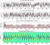 |
Fig. 3 Top panels: fluctuating amplitude of α in the two hemispheres. Middle panel: toroidal field amplitude at r = 0.706 R⊙ and at 14° N (black) and 14° S (red). Bottom panel: corresponding analog to a butterfly diagram. |
3.1. Two poloidal sources at play
Although the previous simulation set-up with fluctuations in a dynamo system with a BL poloidal source alone represents a scenario for entry and exit from grand minima-like conditions, as has been demonstrated in earlier simulations (Charbonneau & Dikpati 2000; Karak 2010; Choudhuri & Karak 2012), the physics of the recovery from a grand minimum in these model set-ups is questionable (Hazra et al. 2014). The problem lies in the parametrization of the BL mechanism itself. Since the main idea behind this mechanism1 is the decay of active regions, one should ensure that this αBL is only acting on strong fields that have buoyantly erupted and not on weaker fields that might reach the surface layers by advection or diffusion. This implies that a lower threshold in the αBL must be introduced to prevent this (Nandy 2002b; Charbonneau et al. 2005; Hazra et al. 2014). Therefore we introduce a new parametrization in the αBL that depends on the field intensity, ![Mathematical equation: \begin{eqnarray} \alpha_{\rm BL} &=& \alpha_{\rm 0BL}\frac{ \cos \theta }{4} \left[1+\textrm{erf} \left( \frac{r-r_1}{d_1}\right)\right] \times\ \left[1-\textrm{erf} \left( \frac{r-r_2}{d_2}\right)\right] \nonumber \\ && \times~ a_1\, \left[ 1 + \textrm{erf} \left(\frac{B_\phi^2 - B_{\rm 1lo}^2}{d_3^2}\right)\right]\times \left[ 1 - \textrm{erf}\left(\frac{B_\phi^2 - B_{\rm 1up}^2}{d_4^2}\right)\right], \label{c6.eq-alphaBL} \end{eqnarray}](/articles/aa/full_html/2014/03/aa22635-13/aa22635-13-eq42.png) (4)where r1, r2, d1, and d2 have the same values as defined for Eq. (3); α0BL controls the amplitude of the effect; a1 = 0.393 is a normalization constant; B1lo = 103 G corresponds to the lower threshold; d3 = 102 G; B1up = 105 G is an upper threshold; and d4 = 106 G. This formulation ensures that only the fields that reach the surface layers with magnitudes between B1lo and B1up contribute to the BL mechanism.
(4)where r1, r2, d1, and d2 have the same values as defined for Eq. (3); α0BL controls the amplitude of the effect; a1 = 0.393 is a normalization constant; B1lo = 103 G corresponds to the lower threshold; d3 = 102 G; B1up = 105 G is an upper threshold; and d4 = 106 G. This formulation ensures that only the fields that reach the surface layers with magnitudes between B1lo and B1up contribute to the BL mechanism.
To determine what would be an appropriate value for the lower threshold of αBL in our model, B1lo, we conducted the following experiment. We performed simulations where we let the model evolve until it reached a maximum concentration of toroidal field in the base of the convection zone (akin to a cycle maximum). In the following step we use this final state as the initial condition of a new simulation and, to ensure that there is no toroidal field in the main body of the convection zone, we added a condition to wipe out fields above r = 0.725 R⊙. In other words, we initiate a new simulation with a high concentration of toroidal field just below the tachocline, but none above. We switched off the buoyancy algorithm and let the dynamo solution evolve just in the presence of advective flows and diffusion. The time that the peak associated with this strong field (~105 G at r = 0.725 R⊙) takes to reach near surface layers at active latitudes, more specifically at a latitude θ = 15° N and r = 0.97 R⊙ around the radius where αBL peaks, is approximately 5 years. The field reaching this radius had an amplitude around 750 G. This implies that this field is being transported primarily by the meridional flow towards the surface. The diffusion timescale for the toroidal field is given by τt = ℓ2/ηt, and direct substitution (ℓ ≃ 0.245 R⊙ and ηt = 4 × 1010 cm2 s-1) yields that τt is around 230 years. Even if we consider an average value of η one order of magnitude higher, we still obtain a diffusion time several times higher than the advection time found.
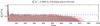 |
Fig. 4 Squared toroidal field amplitude at r = 0.706 R⊙ and θ = 14° N (black) and S (red). In this model set-up with both lower and upper thresholds and fluctuations in the BL mechanism, the dynamo never recovers once it enters a grand minima-like phase. |
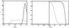 |
Fig. 5 Radial profile (left panel) and quenching profile (right panel) for the Babcock-Leighton αBL (black, solid curves) and for the mean-field αMF (gray, dashed curves). For better visual interpretation, the amplitude in the radial profile of the αMF represented here is scaled up by one order of magnitude above the values used in the simulations. |
This numerical experiment and associated physical insights point out that even if buoyant eruption is absent, for example during solar grand minima episodes, in such model set-ups, the toroidal field is still dredged up from beneath the base of the convection zone to the surface by meridional circulation. Even though this toroidal field takes 5 years to move up and is weak, it ends up at the near-surface region where the spatially distributed, α-coefficient representing the BL poloidal source is located. Not being able to distinguish whether this toroidal field represents a contribution from sunspot eruptions or from dredging up of the field due to meridional circulation, the BL α source ends up producing poloidal fields in a manner that is un-physical and not in keeping with established ideas of the dynamics of magnetic flux tubes. It is well known, that if it takes many years for a toroidal flux tube to rise up, it will be completely shredded by turbulence and will not have the required tilt angle distribution to contribute to the BL mechanism. Thus, to circumvent this un-physical behaviour in the model set-up, a lower threshold of B1lo = 103 G is necessary in such kinematic dynamo models.
The effect of this lower threshold when compared to the reference solution is to lower the amplitude of the solution’s magnetic field and consequently decrease the number of eruptions and the latitudes at which they appear. The value of αBL = 27 now corresponds to a value just above critical with eruptions first appearing at 25 degrees in latitude. This situation makes the dynamo solution especially susceptible to amplitude fluctuations in this coefficient. In Fig. 4 we show a dynamo solution which decays after half a century with just 10% fluctuations in this redefined BL α-coefficient with the lower threshold. The decay time of the solution scales inversely to the fluctuation levels. For the current set-up, fluctuation levels between 50% and 150% induce the decay of the solution after a few decades, but for lower fluctuation level the solution takes more time to decay. The observed decoupling between northern and southern hemispheres that appear in these solutions are also plausibly connected to the fluctuations levels.
Therefore, while a BL mechanism with both upper and a lower operating thresholds allows for the possibility of entering a grand minima period, it does not seem to permit a self-consistent recovery from grand minima episodes; this conclusion is also supported by simulations with the independent, time-delay dynamo model presented in Paper I. Since the Sun has always emerged from such quiescent periods, one needs to come up with a solution that models this behaviour. The solution we present here is inspired by classical αΩ models and its implementation is based on ideas discussed in Paper I in the context of a reduced dynamo model; i.e. we add a weak mean-field α effect working in conjunction with the surface αBL. This αMF operates in the bulk of the convection zone and operates on weak flux tubes that are below a certain threshold and which do not contribute to the formation of sunspots (thus this α effect could be in operation even during grand minima phases).
We parameterize this mean-field α effect as ![Mathematical equation: \begin{eqnarray} \alpha_{\rm MF} &=& \alpha_{\rm 0MF}\frac{ \cos \theta }{4} \left[1+\textrm{erf} \left( \frac{r-r_3}{d_1}\right)\right] \times\ \left[1-\textrm{erf} \left( \frac{r-r_4}{d_2}\right)\right] \nonumber \\ && \times \, \frac{1}{1+\left(\frac{B_\phi}{B_{\rm 2up}}\right)^2}, \end{eqnarray}](/articles/aa/full_html/2014/03/aa22635-13/aa22635-13-eq68.png) (5)where α0MF is the amplitude of the effect, r3 = 0.713 R⊙, r4 = R⊙, and B2up = 104 G is an upper threshold. The radial profile and quenching profiles for the two poloidal sources (parameterized through two α effects as described above) are presented in Fig. 5. The combined final α effect acting in our system is then defined as α = αBL + αMF, the first acting on strong fields that erupt buoyantly to the surface and the second acting on weaker fields that are either advected by meridional flow or diffuse out into the SCZ from the tachocline.
(5)where α0MF is the amplitude of the effect, r3 = 0.713 R⊙, r4 = R⊙, and B2up = 104 G is an upper threshold. The radial profile and quenching profiles for the two poloidal sources (parameterized through two α effects as described above) are presented in Fig. 5. The combined final α effect acting in our system is then defined as α = αBL + αMF, the first acting on strong fields that erupt buoyantly to the surface and the second acting on weaker fields that are either advected by meridional flow or diffuse out into the SCZ from the tachocline.
In the absence of any fluctuations, the solution obtained using this combined α with αBL = 27, B1lo = 103 and αMF = 0.4 is similar to the reference solution (Fig. 2) but with a slight decrease (~1 year) in the period of the cycle and with eruptions starting from somewhat higher latitudes. They are qualitatively similar in other aspects.
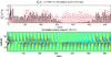 |
Fig. 6 Simulation with αBL = 27 + 100% fluctuations, αMF = 0.4. Between the year 280 and 540, there is a prolonged period without eruptions in the northern hemisphere that is not accompanied by a similar behaviour in the south. |
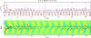 |
Fig. 7 Simulation with αBL = 21 and αMF = 0.4 + 100% fluctuations. Here, the two solar hemispheres appear to be well coupled. |
3.2. Stochastic fluctuations in the poloidal sources
To test if the combination of these two poloidal sources can produce grand minima-like episodes (under the influence of stochastic fluctuations) and recover self-consistently from these episodes, we apply different levels of fluctuations to both α effects, separately and in conjunction to perform further simulations.
We start by repeating the simulation with 100% fluctuations in the αBL = 27, but now with the additional presence of αMF = 0.4 (see Fig. 6). We observe that there are periods when the field falls below the buoyancy threshold, but after some time it regains strength and begins producing sunspot eruptions again. The underlying dynamics probably involves fluctuations in αBL triggering grand minima periods, and the presence of αMF facilitating recovery. Hints of these dynamics between two interacting dynamo α effects were already present in Ossendrijver (2000), but where instead of the near-surface BL α effect, a buoyancy instability induced α effect in the overshoot layer was considered.
In these simulations we continue to observe the decoupling between the northern and southern hemispheres, especially in simulations with a high level of fluctuations in the BL mechanism. Occasionally, small changes in the parity occur as well (deviations from dipolar parity). In some extreme cases, both hemispheres sustain dynamo action but in an almost independent manner. During the deepest phase of a grand minimum the hemispheres loose synchronization, but interestingly it is quickly regained after the system emerges from this quiescent period. There is a small, variable phase shift between the two hemispheres that was already present in Fig. 3. This type of weak hemispheric decoupling during normal activity is plausibly due to the presence of fluctuations and is also observed in the solar butterfly diagram. Different levels of fluctuations in the αBL between 25% and 200% were tested. We observe that the decoupling between hemispheres and the number of grand minima increases with the fluctuation level. Independent simulations in a different context also point out that hemispheric decoupling may be a phenomena that is naturally associated with, and symptomatic of grand minima episodes (Olemskoy & Kitchatinov 2013). In Fig. 6 it can also be seen that, depending on the circumstances, it is possible to have a quiescent minimum-like phase hemisphere, but a failed minimum in the other hemisphere.
In the next batch of simulations we apply fluctuations just to the mean-field poloidal source αMF using a correlation time of 1 year. The simulations with αBL = 27 and αMF = 0.4 + 100% fluctuations returned very few (and short, two cycles at the most) minima episodes. Increasing fluctuations to 200% increases the number of minima, but not their length. To test the importance of αMF in the dynamics, we decrease the strength of the BL source to αBL = 21 (barely supercritical). With this lower value, values of 100% to 200% fluctuations in the mean-field produce longer minima episodes. Both hemispheres seem to evolve in a similar way although some variability between north and south is observed. Even for longer simulated periods, this coupled behaviour is maintained as is the parity of the solution. This implies that the frequency of occurrence, and duration of grand minima episodes depend on the relative amplitudes of the two poloidal sources and the level of fluctuations in them. Moreover, it appears that the mean-field poloidal source – distributed across the convection zone – plays a more important role in the maintenance of hemispheric coupling and dipolar parity than the BL poloidal source.
To complete the set of possible numerical experimentation, different levels of fluctuations can be applied to both the poloidal sources. The overall set of obtained solutions, not surprisingly, shows a wide range of behaviours in terms of frequency and duration of grand minima, hemispheric decoupling, and parity change. A representative solution from numerical simulations with intermittency in both poloidal sources is presented in Fig. 8. Here we note a strong hemispheric asymmetry in the activity just prior to entering the grand minimum phase, continued hemispheric decoupling throughout the minimum phase, and regaining of hemispheric coupling following recovery from the minimum. The period during the grand minimum is characterized by an extended period of low magnetic activity; however, there are occasional sunspot eruptions during this period and the solar polar field (dipolar component) continues its regular cycle of reversal albeit with weak field amplitudes. These features are in broad qualitative agreement with observed features of the solar Maunder minimum (Beer et al. 1998; Miyahara et al. 2006).
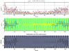 |
Fig. 8 Simulation with αBL = 27 + 100% fluctuations and αMF = 0.4 + 200% fluctuations. The top panel depicts the toroidal field amplitude in the north and south hemispheres; the middle panel is a butterfly diagram for the toroidal field at the base of the convection zone; and the bottom panel shows the radial field near the surface (lighter and darker shades denotes positive and negative radial fields, respectively). This solution, representative of simulations with intermittency in both mean-field and Babcock-Leighton poloidal sources, displays self-consistent entry and exit from grand minima episodes. The butterfly diagram is characterized by hemispheric asymmetry in activity, parity shifts, and occasional sunspot eruptions during the minimum phase. The radial field evolution shows regular polarity reversals in the weak dipolar component of the magnetic field throughout the minimum in activity. |
4. Concluding summary
Solar dynamo models can, in general, explain the main features of the solar cycle. Explanations of solar cycle fluctuations, such as grand minima and maxima episodes, should also be encompassed in these models. Radio-isotope records have shown that our Sun regularly goes through quiescent periods and higher than normal activity phases. To study this activity modulation two different approaches are usually used. In the first approach, one utilizes the role of dynamic, non-linear feedback mechanisms in the solar dynamo (Tobias 1997; Brooke et al. 2002; Bushby 2006) including time delay dynamics (Charbonneau et al. 2005; Wilmot-Smith et al. 2006; Jouve et al. 2010). In the second approach, one utilizes stochastic forcing of the dynamo system motivated from the turbulent nature of the SCZ. In this work we follow the second approach, where we use a stochastically forced kinematic solar dynamo model based on the flux transport paradigm, to focus on solar cycle dynamics related to grand minima episodes.
We also point out that in this model, turbulent diffusion, and not meridional circulation, is the dominant process for transporting the poloidal field in the solar interior where the toroidal field is produced and stored. However, meridional circulation does play an important role in the near-surface poloidal field dynamics and latitudinal transport of toroidal fields deep in the interior. In this context it should be noted that another mechanism, downward turbulent pumping of magnetic flux (Tobias 2001), is also expected to play an important role in solar cycle dynamics (Guerrero & de Gouveia Dal Pino 2008; Nandy & Karak 2012). Moreover, turbulent pumping in a rotating medium may also contribute to the reprocessing of magnetic flux and thus be an effective mechanism for the continuation of weak cycles; we expect that the current model set-up with a mean-field α effective on weak fields would encompass the consequences of such a mechanism implicitly, even in the absence of an explicit treatment of turbulent pumping.
Since the convection zone is highly turbulent, stochastic fluctuations arise naturally in the dynamo source terms. Motivated by the results obtained in a low-order dynamo system in Paper I, showing the importance of a dual source formalism in the context of self-consistent entry and exit from grand minima, we started by adding a lower quenching threshold to the parametrization of the BL poloidal source. Adding this low-threshold to the Babcock-Leighton mechanism ensures that this source only acts on strong fields that erupt to the surface and not on weak fields that leak into the convection zone by advection and diffusion. These weak fields do not produce sunspots, hence they do not participate in the BL mechanism. We believe that this presents a more realistic approach to modelling the BL poloidal source. Although stochastic fluctuations (in αBL) in models without the lower threshold present grand minima like episodes, we argue that these are not real and are un-physical. When the threshold is included, the model returns solutions with a weaker amplitude of the magnetic field that are very susceptible to stochastic fluctuations and models with this physically justified BL source parametrization fail to recover from a grand minima as pointed out in Paper I.
An additional weak, classical mean-field effect, αMF, operating in the bulk of the convection zone is introduced in the model. This source acts on toroidal fields that are not strong enough to produce sunspots and are advected by the meridional flow (and diffuses) into the convection zone. Our kinematic dynamo model with the dual poloidal sources presents typical dynamo solutions with emerging patterns similar to the classical sunspot butterfly diagram. This model presents more robust solutions when stochastic fluctuations are introduced to both α effects (separately or simultaneously). For several combinations in the parameter space, we observe behaviours analogous to grand minima, where the eruption of toroidal fields at the surface is suppressed. However, with this dual poloidal source, physically consistent recovery from a grand minimum is possible as demonstrated in this spatially extended dynamo model. Thus, the results obtained herein corroborate and extend those already presented in Paper I (using a completely different modelling technique), which justifies the usage of appropriate low-order models such as the time delay dynamo model used in Paper I to explore long-term phenomena which are computationally expensive for spatially extended dynamo models.
Two possible scenarios for entering and exiting a grand minimum were identified. The first is the case where small fluctuations in the surface αBL are combined with fluctuations in αMF in a model with a near critical solution. Since the field is near the limit necessary for the production of sunspots, fluctuations in αMF can take it below the buoyancy threshold. These grand minima tend to be small with a duration of just a few cycles. The other case is in models with solutions above critical when both source terms are subjected to considerable levels of fluctuation (above 75%). In this case, fluctuations in αBL tend to make the toroidal field fall abruptly below the threshold necessary for the production of sunspot eruptions; this renders the BL source completely ineffective with consequent disruption of dynamo activity. The combination of different fluctuation levels also controls the onset of the grand minima (abrupt or gradual). In several cases we observe that one of the hemispheres emerges from a minimum a few cycles before the other. This was also apparently the case during the exit from the Maunder minimum (Nagovitsyn et al. 2010), so this model behaviour is entirely plausible.
We find that fluctuations in αBL tend to decouple the magnetic activity in the two hemispheres as observed in these spatially extended simulations because in our model we allow for different randomly generated fluctuations in the northern and southern hemispheres, which is expected in reality. Nevertheless, for fluctuations of αBL of the order of 25% the asymmetry between hemispheric magnetic activity is small, but with increasing fluctuation levels this asymmetry increases. We find that the mean-field poloidal source plays a more important role in keeping the two hemispheres coupled, while fluctuations in the BL source tends to introduce parity shifts and decouple the two hemispheres. It is possible, as demonstrated, that under certain conditions, one hemisphere may undergo minimum like conditions with no eruptions while there is a failed minimum in the other hemisphere where sunspot eruptions continue. Independent simulations point out that hemispheric asymmetry may be symptomatic of grand minima episodes; Olemskoy & Kitchatinov (2013) and Charbonneau et al. (2005) provide a possible physical explanation of the role of hemispheric coupling vis-a-vis solar grand minima episodes.
We note that for a large number of combinations of poloidal source amplitudes and fluctuations, we see regular polar field reversals (in radial field evolution) even when the surface BL mechanism remains ineffective over a long period during a grand minimum (because of the lack of bipolar sunspot eruptions). This behaviour in our model is due to the presence of the mean-field poloidal source which maintains a low activity cycles. This result is supported by solar activity reconstructions based on cosmogenic isotopes which indicate regular polar field reversals occurred during the Maunder minimum (Miyahara et al. 2004).
One of the important aspects of extreme solar activity fluctuations is the observed statistics (i.e. the frequency distribution) of solar grand minima and maxima episodes (Usoskin et al. 2007). These constraints are on the duration and waiting periods for minima and maxima episodes. While we have not addressed this aspect in our first comprehensive study with a dynamo driven by dual poloidal field sources, we point out that an independent study does focus on a comparative analysis of the observed statistics of grand minima with a kinematic dynamo model set-up in a similar way (Karak & Choudhuri 2013). Another important aspect that we do not directly focus on here is the phase that immediately precedes a solar grand minimum and the defining characteristics of this phase. Since such studies require detailed investigations, and significant computational investment in simulations, we defer this to the future.
Henceforth we will use the subscript BL to denote the Babcock-Leighton α effect and MF for the classical mean-field α effect.
Acknowledgments
We are grateful to the Ministry of Human Resource Development, Council for Scientific and Industrial Research, University Grants Commission and the Ramanujan Fellowship award of the Department of Science and Technology of the Government of India for supporting this research. D. Passos acknowledges support from the Fundação para a Ciência e Tecnologia grant SFRH/BPD/68409/2010, CENTRA-IST, the University of the Algarve for providing office space and he is also grateful to IISER Kolkata for hosting him during the final phases of the research work presented here. We also acknowledge the referee for his critical comments which helped us improve an earlier version of our manuscript.
References
- Babcock, H. W., & Babcock, H. D. 1955, ApJ, 121, 349 [NASA ADS] [CrossRef] [Google Scholar]
- Beaudoin, P., Charbonneau, P., Racine, E., & Smolarkiewicz, P. K. 2012, Sol. Phys., 282, 335 [Google Scholar]
- Beer, J., Tobias, S. M., & Weiss, N. O. 1998, Sol. Phys., 181, 237 [Google Scholar]
- Brandenburg, A., & Spiegel, E. A. 2008, Astron. Nachr., 329, 351 [NASA ADS] [CrossRef] [Google Scholar]
- Brandenburg, A., Radler, K.-H., Rheinhardt, M., & Käpylä, P. J. 2008, ApJ, 676, 740 [NASA ADS] [CrossRef] [Google Scholar]
- Brooke, J., Moss, D., & Phillips, A. 2002, A&A, 395, 1013 [NASA ADS] [CrossRef] [EDP Sciences] [Google Scholar]
- Brown, B. P., Browning, M. K., Brun, A. S., Miesch, M. S., & Toomre, J. 2010, ApJ, 711, 424 [Google Scholar]
- Bushby, P. J. 2006, MNRAS, 371, 772 [Google Scholar]
- Caligari, P., Moreno-Insertis, F., & Schüssler, M. 1995, ApJ, 441, 886 [NASA ADS] [CrossRef] [Google Scholar]
- Charbonneau, P. 2010, Liv. Rev. Sol. Phys., 7, 3 [Google Scholar]
- Charbonneau, P., & Dikpati, M. 2000, ApJ, 543, 1027 [NASA ADS] [CrossRef] [Google Scholar]
- Charbonneau, P., Blais-Laurier, G., & St-Jean, C. 2004, ApJ, 616, 183 [Google Scholar]
- Charbonneau, P., St-Jean, C., & Zacharias, P. 2005, ApJ, 619, 613 [NASA ADS] [CrossRef] [Google Scholar]
- Chatterjee, P., Nandy, D., & Choudhuri, A. R. 2004, A&A, 427, 1019 [NASA ADS] [CrossRef] [EDP Sciences] [Google Scholar]
- Choudhuri, A. R. 1992, A&A, 253, 277 [NASA ADS] [Google Scholar]
- Choudhuri, A. R., & Karak, B. B. 2012, Phys. Rev. Lett., 109, 171103 [NASA ADS] [CrossRef] [Google Scholar]
- Dasi-Espuig, M., Solanki, S. K., Krivova, N., Cameron, R., & Peñuela, T. 2010, A&A, 518, A10 [Google Scholar]
- Dikpati, M., & Charbonneau, P. 1999, ApJ, 518, 508 [NASA ADS] [CrossRef] [Google Scholar]
- Durney, B. R. 1995, Sol. Phys., 160, 213 [Google Scholar]
- D’Silva, S., & Choudhuri, A. 1993, A&A, 272, 621 [NASA ADS] [Google Scholar]
- Eddy, J. A. 1976, Science, 192, 1189 [NASA ADS] [CrossRef] [PubMed] [Google Scholar]
- Fan, Y. 2001, ApJ, 554, 111 [Google Scholar]
- Guerrero, G., & de Gouveia Dal Pino, E. M. 2008, A&A, 485, 267 [NASA ADS] [CrossRef] [EDP Sciences] [Google Scholar]
- Haigh, J. D. 2007, Liv. Rev. Sol. Phys., 4, 2 [Google Scholar]
- Hazra, S., Passos, D., & Nandy, D. 2014, ApJ, submitted [arXiv:1307.5751v3] [Google Scholar]
- Hoyng, P. 1988, ApJ, 332, 857 [NASA ADS] [CrossRef] [Google Scholar]
- Hoyng, P. 1993, A&A, 272, 321 [NASA ADS] [Google Scholar]
- Hoyng, P., Schmitt, D., & Teuben, L. J. W. 1994, A&A, 289, 265 [NASA ADS] [Google Scholar]
- Howard, R. F. 1991, Sol. Phys., 136, 251 [Google Scholar]
- Jouve, L., Proctor, M. R. E., & Lesur, G. 2010, A&A, 519, A13 [Google Scholar]
- Käpylä, P. J., Korpi, M. J., Ossendrijver, M., & Stix, M. 2006, A&A, 455, 401 [NASA ADS] [CrossRef] [EDP Sciences] [Google Scholar]
- Karak, B. 2010, ApJ, 724, 1021 [NASA ADS] [CrossRef] [Google Scholar]
- Karak, B., & Choudhuri, A. R. 2013, Res. Astron. Astrophys., 13, 1339 [NASA ADS] [CrossRef] [Google Scholar]
- Leighton, R. B. 1969, ApJ, 156, 1 [Google Scholar]
- Lopes, I., & Passos, D. 2009, Sol. Phys., 257, 1 [NASA ADS] [CrossRef] [Google Scholar]
- Maunder, E. W. 1904, MNRAS, 64, 747 [NASA ADS] [Google Scholar]
- Miyahara, H., Masuda, K., Muraki, Y., et al. 2004, Sol. Phys., 224, 317 [Google Scholar]
- Miyahara, H., Masuda, K., Muraki, Y., Kitagawa, H., & Nakamura, T. 2006, J. Geophys. Res., 111, A03103 [NASA ADS] [CrossRef] [Google Scholar]
- Moss, D., Sokoloff, D., Usoskin, I., & Tutubalin, V. 2008, Sol. Phys., 250, 221 [NASA ADS] [CrossRef] [Google Scholar]
- Nandy, D. 2002, Ap&SS, 282, 209 [NASA ADS] [CrossRef] [Google Scholar]
- Nandy, D., & Choudhuri, A. R. 2002, Science, 296, 1671 [NASA ADS] [CrossRef] [PubMed] [Google Scholar]
- Nandy, D., & Karak, B. 2012, AAS Meeting, 220, 521.18 [Google Scholar]
- Nagovitsyn, Y. A., Ivanov, V. G., Miletsky, E. V., & Nagovitsyna, E. Y. 2010, Astron. Rep., 54, 476 [NASA ADS] [CrossRef] [Google Scholar]
- Olemskoy, S. V., & Kitchatinov, L. L. 2013, ApJ, 777, 71 [Google Scholar]
- Ossendrijver, M. A. J. H. 2000, A&A, 359, 364 [NASA ADS] [Google Scholar]
- Owens, B. 2013, Nature 495, 300 [Google Scholar]
- Parker, E. N. 1955, ApJ, 121, 491 [NASA ADS] [CrossRef] [Google Scholar]
- Passos, D., Charbonneau, P., & Beaudoin, P. 2012, Sol. Phys., 279, 1 [Google Scholar]
- Proctor, M. R. E. 2007, MNRAS, 382, 39 [NASA ADS] [CrossRef] [Google Scholar]
- Racine, E., Charbonneau, P., Ghizaru, M., Bouchat, A., & Smolarkiewicz, P. K. 2011, ApJ, 735, 46 [NASA ADS] [CrossRef] [Google Scholar]
- Rempel, M. 2006, ApJ, 647, 662 [NASA ADS] [CrossRef] [Google Scholar]
- Steinhilber, F., Abreu., J., Beer, J., et al. 2012, PNAS, 109, 5967 [Google Scholar]
- Steenbeck, M., Krause, F., & Rädler, K.-H. 1966, Z. Naturforsch, 21, 1285 [Google Scholar]
- Tobias, S. M. 1996, ApJ, 467, 870 [NASA ADS] [CrossRef] [Google Scholar]
- Tobias, S. M. 1997, A&A, 322, 1007 [NASA ADS] [Google Scholar]
- Tobias, S. M. 2002, Astron. Nachr., 323, 417 [Google Scholar]
- Tobias, S. M., Brummell, N. H., Clune, T. L., & Toomre, J. 2001, ApJ, 549, 1183 [NASA ADS] [CrossRef] [Google Scholar]
- Usoskin, I. 2008, Liv. Rev. Sol. Phys., 5, 3 [Google Scholar]
- Usoskin, I., Solanki, S., & Kovaltsov, G. 2007, A&A, 471, 301 [NASA ADS] [CrossRef] [EDP Sciences] [Google Scholar]
- Wang, Y.-M., Sheeley, N. R., & Nash, A. G. 1991, ApJ, 383, 431 [NASA ADS] [CrossRef] [Google Scholar]
- Wilmot-Smith, A. L., Nandy, D., Hornig, G., & Martens, P. C. H. 2006, ApJ, 652, 696 [NASA ADS] [CrossRef] [Google Scholar]
- Yeates, A. R., Nandy, D., & Mackay, D. H. 2008, ApJ, 673, 544 [NASA ADS] [CrossRef] [Google Scholar]
All Figures
|
Fig. 1 Left panel: shows the toroidal (dashed) and poloidal (solid) magnetic diffusivity profiles. Right panel: radial profile of the α coefficient that is used to model the near-surface BL poloidal source (in m s-1). |
| In the text | |
|
Fig. 2 Top panel: toroidal field amplitude, |
| In the text | |
|
Fig. 3 Top panels: fluctuating amplitude of α in the two hemispheres. Middle panel: toroidal field amplitude at r = 0.706 R⊙ and at 14° N (black) and 14° S (red). Bottom panel: corresponding analog to a butterfly diagram. |
| In the text | |
|
Fig. 4 Squared toroidal field amplitude at r = 0.706 R⊙ and θ = 14° N (black) and S (red). In this model set-up with both lower and upper thresholds and fluctuations in the BL mechanism, the dynamo never recovers once it enters a grand minima-like phase. |
| In the text | |
|
Fig. 5 Radial profile (left panel) and quenching profile (right panel) for the Babcock-Leighton αBL (black, solid curves) and for the mean-field αMF (gray, dashed curves). For better visual interpretation, the amplitude in the radial profile of the αMF represented here is scaled up by one order of magnitude above the values used in the simulations. |
| In the text | |
|
Fig. 6 Simulation with αBL = 27 + 100% fluctuations, αMF = 0.4. Between the year 280 and 540, there is a prolonged period without eruptions in the northern hemisphere that is not accompanied by a similar behaviour in the south. |
| In the text | |
|
Fig. 7 Simulation with αBL = 21 and αMF = 0.4 + 100% fluctuations. Here, the two solar hemispheres appear to be well coupled. |
| In the text | |
|
Fig. 8 Simulation with αBL = 27 + 100% fluctuations and αMF = 0.4 + 200% fluctuations. The top panel depicts the toroidal field amplitude in the north and south hemispheres; the middle panel is a butterfly diagram for the toroidal field at the base of the convection zone; and the bottom panel shows the radial field near the surface (lighter and darker shades denotes positive and negative radial fields, respectively). This solution, representative of simulations with intermittency in both mean-field and Babcock-Leighton poloidal sources, displays self-consistent entry and exit from grand minima episodes. The butterfly diagram is characterized by hemispheric asymmetry in activity, parity shifts, and occasional sunspot eruptions during the minimum phase. The radial field evolution shows regular polarity reversals in the weak dipolar component of the magnetic field throughout the minimum in activity. |
| In the text | |
Current usage metrics show cumulative count of Article Views (full-text article views including HTML views, PDF and ePub downloads, according to the available data) and Abstracts Views on Vision4Press platform.
Data correspond to usage on the plateform after 2015. The current usage metrics is available 48-96 hours after online publication and is updated daily on week days.
Initial download of the metrics may take a while.