| Issue |
A&A
Volume 562, February 2014
|
|
|---|---|---|
| Article Number | A145 | |
| Number of page(s) | 10 | |
| Section | Extragalactic astronomy | |
| DOI | https://doi.org/10.1051/0004-6361/201322510 | |
| Published online | 24 February 2014 | |
Search for extended γ-ray emission around AGN with H.E.S.S. and Fermi-LAT
1
Universität Hamburg, Institut für
Experimentalphysik, Luruper Chaussee
149, 22761
Hamburg,
Germany
2
Max-Planck-Institut für Kernphysik, PO Box 103980, 69029
Heidelberg,
Germany
3
Dublin Institute for Advanced Studies,
31 Fitzwilliam place,
Dublin 2,
Ireland
4
National Academy of Sciences of the Republic of
Armenia, Yerevan,
Armenia
5
Yerevan Physics Institute, 2 Alikhanian Brothers St., 375036
Yerevan,
Armenia
6
Institut für Physik, Humboldt-Universität zu Berlin,
Newtonstr. 15, 12489
Berlin,
Germany
7
Universität Erlangen-Nürnberg, Physikalisches
Institut, Erwin-Rommel-Str.
1, 91058
Erlangen,
Germany
8
University of Namibia, Department of Physics,
Private Bag
13301, Windhoek, Namibia
9
University of Durham, Department of Physics,
South Road, Durham
DH1 3LE,
UK
10
DESY, 15738
Zeuthen,
Germany
11
Institut für Physik und Astronomie, Universität
Potsdam, Karl-Liebknecht-Strasse
24/25, 14476
Potsdam,
Germany
12
Nicolaus Copernicus Astronomical Center,
ul. Bartycka 18, 00-716
Warsaw,
Poland
13
Department of Physics and Electrical Engineering, Linnaeus
University, 351
95
Växjö,
Sweden
14
Institut für Theoretische Physik, Lehrstuhl IV: Weltraum und
Astrophysik, Ruhr-Universität Bochum, 44780
Bochum,
Germany
15
Institut für Astro- und Teilchenphysik,
Leopold-Franzens-Universität Innsbruck, 6020
Innsbruck,
Austria
16
Laboratoire Leprince-Ringuet, Ecole Polytechnique,
CNRS/IN2P3, 91128
Palaiseau,
France
17
Now at Santa CruzInstitute for Particle Physics, Department of
Physics, University of California at Santa Cruz, Santa Cruz
CA
95064,
USA
18
Centre for Space Research, North-West University,
Potchefstroom
2520, South
Africa
19
LUTH, Observatoire de Paris, CNRS, Université Paris
Diderot, 5 place Jules
Janssen, 92190
Meudon,
France
20
LPNHE, Université Pierre et Marie Curie Paris 6, Université Denis
Diderot Paris 7, CNRS/IN2P3, 4
place Jussieu, 75252, Paris Cedex
5, France
21
Institut für Astronomie und Astrophysik, Universität
Tübingen, Sand 1,
72076
Tübingen,
Germany
22
DSM/Irfu, CEA Saclay, 91191
Gif-Sur-Yvette Cedex,
France
23
Astronomical Observatory, The University of Warsaw,
Al. Ujazdowskie 4, 00-478
Warsaw,
Poland
24
School of Physics, University of the Witwatersrand,
1 Jan Smuts avenue, Braamfontein,
2050
Johannesburg, South
Africa
25
Landessternwarte, Universität Heidelberg,
Königstuhl, 69117
Heidelberg,
Germany
26
Oskar Klein Centre, Department of Physics, Stockholm University,
Albanova University Center, 10691
Stockholm,
Sweden
27
Wallenberg Academy Fellow
28
Université Bordeaux 1, CNRS/IN2P3, Centre d’Études Nucléaires de
Bordeaux-Gradignan , 33175
Gradignan,
France
29
Funded by contract ERC-StG-259391 from the European Community
30
School of Chemistry & Physics, University of
Adelaide, 5005
Adelaide,
Australia
31
APC, AstroParticule et Cosmologie, Université Paris Diderot,
CNRS/IN2P3, CEA/Irfu, Observatoire de Paris, Sorbonne Paris Cité,
10 rue Alice Domon et Léonie
Duquet, 75205
Paris Cedex 13,
France
32
UJF-Grenoble 1/CNRS-INSU, Institut de Planétologie et
d’Astrophysique de Grenoble (IPAG) UMR 5274, 38041
Grenoble,
France
33
Department of Physics and Astronomy, The University of Leicester,
University road, Leicester
LE1 7RH,
UK
34
Instytut Fizyki Jądrowej PAN, ul. Radzikowskiego 152, 31-342
Kraków,
Poland
35
Laboratoire Univers et Particules de Montpellier, Université
Montpellier 2, CNRS/IN2P3, CC 72,
place Eugène Bataillon, 34095
Montpellier Cedex 5,
France
36
Laboratoire d’Annecy-le-Vieux de Physique des Particules,
Université de Savoie, CNRS/IN2P3, 74941
Annecy-le-Vieux,
France
37
Obserwatorium Astronomiczne, Uniwersytet
Jagielloński, ul. Orla
171, 30-244
Kraków,
Poland
38
Toruń Centre for Astronomy, Nicolaus Copernicus
University, ul. Gagarina
11, 87-100
Toruń,
Poland
39
Department of Physics, University of the Free State,
PO Box 339, Bloemfontein
9300, South
Africa
40 Charles University, Faculty of
Mathematics and Physics, Institute of Particle and Nuclear Physics,
V Holešovičkách 2, 180 00
Prague 8, Czech
Republic
Received: 20 August 2013
Accepted: 12 January 2014
Context. Very-high-energy (VHE; E > 100 GeV) γ-ray emission from blazars inevitably gives rise to electron-positron pair production through the interaction of these γ-rays with the extragalactic background light (EBL). Depending on the magnetic fields in the proximity of the source, the cascade initiated from pair production can result in either an isotropic halo around an initially beamed source or a magnetically broadened cascade flux.
Aims. Both extended pair-halo (PH) and magnetically broadened cascade (MBC) emission from regions surrounding the blazars 1ES 1101-232, 1ES 0229+200, and PKS 2155-304 were searched for using VHE γ-ray data taken with the High Energy Stereoscopic System (H.E.S.S.) and high-energy (HE; 100 MeV < E < 100 GeV) γ-ray data with the Fermi Large Area Telescope (LAT).
Methods. By comparing the angular distributions of the reconstructed γ-ray events to the angular profiles calculated from detailed theoretical models, the presence of PH and MBC was investigated.
Results. Upper limits on the extended emission around 1ES 1101-232, 1ES 0229+200, and PKS 2155-304 are found to be at a level of a few per cent of the Crab nebula flux above 1 TeV, depending on the assumed photon index of the cascade emission. Assuming strong extra-Galactic magnetic field (EGMF) values, >10-12 G, this limits the production of pair haloes developing from electromagnetic cascades. For weaker magnetic fields, in which electromagnetic cascades would result in MBCs, EGMF strengths in the range (0.3−3)× 10-15 G were excluded for PKS 2155-304 at the 99% confidence level, under the assumption of a 1 Mpc coherence length.
Key words: gamma rays: galaxies / galaxies: magnetic fields / intergalactic medium / BL Lacertae objects: individual: PKS 2155-304 / BL Lacertae objects: individual: 1ES 1101-232 / BL Lacertae objects: individual: 1ES 0229+200
© ESO, 2014
EGMF strength regimes for no-cascade, pair-halo, and MBC development.
1. Introduction
About 50 active galactic nuclei1(AGN) with redshifts ranging from 0.002 to 0.6 have so far been detected in very-high-energy (VHE; E > 100 GeV) γ-rays. Significant emission beyond TeV energies has been measured for half of them. The spectra of such TeV-bright AGN with redshifts beyond z ~ 0.1 are significantly affected by the extragalactic background light (EBL; Nikishov 1962; Jelley 1966; Gould & Schréder 1966), with the γ-rays from these sources interacting with the EBL and generating electron-positron pairs. The pairs produced, in turn, are deflected by the extra-Galactic magnetic field (EGMF) and cooled by interacting both with the EGMF via the synchrotron effect and with the cosmic microwave background (CMB) via the inverse Compton (IC) effect. Thus, cascades can develop under certain conditions, with the emerging high-energy photons being unique carriers of information about both the EBL (Stecker & de Jager 1993) and EGMF (Neronov & Semikoz 2009).
Should the electron-positron pairs pass the bulk of their energy into the background plasma through the growth of plasma instabilities (Broderick et al. 2012), a high-energy probe of the EGMF could be invalidated. The growth rate of such instabilities, however, remains unclear and is under debate (Schlickeiser et al. 2012; Miniati & Elyiv 2013). This work is conducted under the premise that the IC cooling channel of the pairs dominates any plasma cooling effects.
The strength of the EGMF has a major impact on the development of the cascades. To explain its effects, three regimes of EGMF strength are introduced in Table 1. For strong magnetic fields (>10-7 G, regime I), synchrotron cooling of pair-produced electrons becomes non-negligible, suppressing the production of secondary γ-rays (Gould & Rephaeli 1978). For such a scenario, the observed, Jobs., and intrinsic, J0, γ-ray fluxes are related as Jobs.(E) = J0(E)exp [−τγγ(E,z)]. Here, τγγ(E,z) is the pair-production optical depth, which depends on the photon energy E and the redshift of the source z, as well as on the level of the EBL flux F(λ,z), where λ is the EBL wavelength.
A weaker EGMF assumption removes the simple relation between the observed and intrinsic energy spectra. For magnetic field strengths between 10-7 G and 10-12 G (regime II), the electron pairs produced are isotropised and accumulate around the source, eventually giving rise to a pair halo of secondary γ-rays (Aharonian et al. 1994). Since the isotropisation takes place on much smaller scales than the cooling, the size of this pair halo depends mainly upon the pair-production length, with very little variation being introduced by the actual strength of the EGMF in the above-mentioned range. The observed flux thus consists of both primary and secondary high-energy γ-rays, and its relation to the intrinsic spectrum cannot be reduced to the simple effect of absorption described by the optical depth (e.g., Taylor et al. 2011; Essey et al. 2011). Furthermore, the level of secondary γ-rays emitted by the population of accumulated pairs within the halo is able to provide a natural record of the AGNs past activity (Aharonian et al. 1994).
Unfortunately, owing to the low γ-ray flux of the sources, and/or a possible cut-off in the spectra below 10 TeV, combined with the limited sensitivity of current-generation γ-ray telescopes, the detection of these haloes in VHE γ-rays cannot be guaranteed. Because of strong Doppler boosting, the apparent γ-ray luminosities of AGN can significantly exceed the intrinsic source luminosity (Lind & Blandford 1985). Furthermore, leptonic models for many of the currently observed blazars do not require high photon fluxes beyond 10 TeV.
For even weaker magnetic field values (regime III, B < 10-14 G), no pair halo is formed, and the particle cascade continues to propagate along the initial beam direction, broadening the beam width. The angular size of this magnetically broadened cascade (MBC) is dictated by the EGMF strength, and a measurement of the broadened width can provide a strong constraint on the EGMF value. Complementary to this probe, the combined spectra of the TeV and GeV γ-ray emission observed from a blazar can also be used as a probe of the intervening EGMF, as demonstrated in Neronov & Vovk (2010), Taylor et al. (2011), and Arlen et al. (2012). Although generally the intergalactic magnetic field is expected to have a much higher value, current observations and cosmological concepts cannot exclude that in so-called “voids”, with sizes as large as 100 Mpc, the magnetic field can be as small as 10-17 G (Miniati & Bell 2011; Durrer & Neronov 2013). In the case of such weak “void” fields, instead of persistent isotropic pair halo emission, the observer would see direct cascade emission propagating almost rectilinearly over cosmological distances.
As for the case of pair haloes, the arriving flux in MBCs is also naturally expected to consist of a mixture of primary and secondary γ-rays. For flat or soft intrinsic spectra (i.e., photon indices Γ ≳ 2), cascade photons are expected to constitute a sub-dominant secondary component, making measurements of the EBL imprint in blazar spectra possible (Aharonian et al. 2007a; H.E.S.S. Collaboration 2013; Meyer et al. 2012). If, in contrast, the primary spectrum of γ-rays is hard and extends beyond 10 TeV, then, at lower energies, the secondary radiation can even dominate the primary γ-ray component. Thus, in this case, the deformation of the γ-ray spectrum due to absorption would be more complex than in the case discussed above.
In a very small magnetic field, cascades initiated at very high energies lead to the efficient transfer of energy back and forth between the electron and γ-ray components, effectively reducing the γ-ray opacity in the energy range of secondary particles (Aharonian et al. 2002; Essey et al. 2011). As a result, the observer is able to see γ-rays at energies for which τγγ ≫ 1.
On the other hand, deflections in the EGMF mean that the original γ-ray beam is broadened, and even extremely low EGMF values (~10-15 G) are expected to produce detectable extended γ-ray emission. This radiation should be clearly distinguished from that of pair haloes. The origin of the extended emission in these two cases is quite different, with pair haloes producing extended emission isotropically and MBCs producing extended emission only in the jet direction.
The radiation from both pair haloes and MBCs can be recognised by a distinct variation in intensity with angular distance from the centre of the blazar. This variation is expected to depend weakly on the orientation and opening angle of the jet, and more on the total luminosity and duty cycle of the source at energies ≥10 TeV (Aharonian et al. 1994). To a first-order approximation, the radiation deflection angles remain small in comparison to the angular size of the jet. Since the observer remains “within the jet”, the angles (relative to the blazar direction) from which the observer can receive the magnetically broadened emission remain roughly independent of the observer’s exact position within the jet cone. This result, however, only holds true if the observer is not too close to the edge of the jet.
The preferred distance for observing both pair haloes and MBCs with the H.E.S.S. experiment is in the range of hundreds of mega-parsecs to around one giga-parsec, i.e. in the range of ~0.1 to ~0.24 in redshift. The far limit is set by the reduction in flux with distance down to a limit that is only just sufficient for detection. The near limit for pair haloes results from the fact that for sources that are too close, it becomes impossible to distinguish between their halo photons and background radiation, since the halo would take up the entire field of view of the observing instrument, i.e. 5° for H.E.S.S. For MBCs, similar near and far limits are found. In this case, however, the near limit comes purely from a lack of cascade luminosity: it only becomes significant for distances beyond several pair production lengths.
A first search for pair-halo emission was conducted by the HEGRA collaboration (Aharonian et al. 2001) using Mkn 501 observations (z = 0.033). This yielded an upper limit of (5−10)% of the Crab nebula flux (at energies ≥1 TeV) on angular scales of 0.5° to 1° from the source. The MAGIC collaboration performed a similar search for extended emission using Mkn 421 and Mkn 501 (Aleksić et al. 2010). Upper limits on the extended emission around Mkn 421 at a level of <5% of the Crab nebula flux were obtained and a value of <4% of the Crab nebula flux was achieved for Mkn 501, both above an energy threshold of 300 GeV. These results were used to exclude EGMF strengths in the range of a few times 10-15 G. Since both Mkn 421 and Mkn 501 are very close by, the extension of the halo emission is expected to be large. There are therefore no ideal candidates for this work.
More recently, a study was performed using data from the Fermi Large Area Telescope (LAT) (Ando & Kusenko 2010). Images from the 170 brightest AGN in the 11-month Fermi source catalogue were stacked together. Evidence has been claimed for MBCs in the form of an excess over the point-spread function with a significance of 3.5σ. However, Neronov et al. (2011) show that the angular distribution of γ-rays around the stacked AGN sample is consistent with the angular distribution of the γ-rays around the Crab nebula, (which is a point-like source for Fermi) indicating systematic problems with the LAT point spread function (PSF).
In the latest publication on this topic (Ackermann et al. 2013), pair-halo emission around AGN detected with Fermi-LAT was investigated with an updated PSF. A sample of 115 BL Lac-type AGN was divided into high- (z > 0.5) and low-redshift (z < 0.5) blazars, and their stacked angular profiles were tested for disk and Gaussian-shaped pair-halo emission with extensions of 0.1°, 0.5°, and 1.0° by employing a maximum likelihood analysis in angular bins. No evidence of pair-halo emission was found in contrast to the results presented in Ando & Kusenko (2010), and upper limits on the fraction of pair-halo emission relative to the source flux are given for three energy bins in the stacked samples. Additionally, for 1ES 0229+200 and 1ES 0347-121, two BL Lac objects that show γ-ray emission at TeV energies, upper limits on the energy flux assuming different pair-halo radii are given for energies between 1 and 100 GeV.
In this paper, a search for TeV γ-ray pair haloes and MBCs surrounding known VHE γ-ray sources is presented. This study utilises both Fermi-LAT and H.E.S.S. data from three blazars. The three AGN selected, 1ES 1101-232, 1ES 0229+200, and PKS 2155-304, were observed between 2004 and 2009 with H.E.S.S. These AGN are in the preferable redshift range and have emission extending into the multi-TeV energy domain, thus making them ideal candidates for this study.
2. Data sets and analyses
2.1. H.E.S.S. observations and analysis methods
The H.E.S.S. experiment is located in the Khomas Highland of Namibia (23°16′18′′S, 16°30′0′′E), 1835 m above sea level (Hinton 2004). From January 2004 to July 2012, it was operated as a four-telescope array (phase-I). The Imaging Atmospheric Cherenkov Telescopes (IACT) from this phase are in a square formation with a side length of 120 m. They have an effective mirror area of 107 m2, detect cosmic γ-rays in the 100 GeV to 100 TeV energy range and cover a field of view of 5° in diameter. In July 2012, a fifth telescope, placed in the middle of the original square, started taking data (phase-II). With its 600 m2 mirror area, H.E.S.S. will be sensitive to energies as low as several tens of GeV.
For this analysis, only data from H.E.S.S. phase-I were used. To improve the angular
resolution, only observations made with all four phase-I telescopes were included.
Standard H.E.S.S. data quality selection criteria (Aharonian et al. 2006) were applied to the data set of each source. All data
passing the selection were processed using the standard H.E.S.S. calibration (Aharonian et al. 2004). Standard cuts
(Benbow 2005) were used for the event
selection and the data was analysed with the H.E.S.S. analysis package (HAP, version
10-06). The reflected region method (Aharonian et al. 2006) was used to estimate the γ-ray like background.
Circular regions with a radius of  around the sources were excluded from
background estimation in order to avoid a possible contamination by extended emission from
pair haloes or MBCs.
around the sources were excluded from
background estimation in order to avoid a possible contamination by extended emission from
pair haloes or MBCs.
The significance (in standard deviations, σ) of the observed excess was calculated following Li & Ma (1983). All upper limits are derived following the method of Feldman & Cousins (1998).
Using the stereoscopic array of four IACTs, the PSF is characterised by a 68% containment radius of ~0.1 degrees (Aharonian et al. 2006). The distribution of the squared angular distance between the reconstructed shower position and the source position (θ2) for a point-like source peaks at θ2 = 0 and displays the PSF width. The PSF is calculated from Monte-Carlo simulations, taking the observation conditions (e.g. the zenith angle and the optical efficiency of the system) of each observation into account, as well as the photon index of the source.
Summary of the H.E.S.S. analysis results for 1ES 1101-232, 1ES 0229+200 and PKS 2155-304.
Three VHE γ-ray sources, 1ES 1101-232, 1ES 0229+200, and PKS 2155-304, have been chosen for this study due to their strong emission in the >TeV energy range and their location in the suitable redshift range. With ~170 hours of good quality data, PKS 2155-304 is a particularly well suited candidate for this investigation. A summary of the results from the analyses can be found in Table 2. The results presented below have been cross-checked with an independent analysis, the Model Analysis (de Naurois & Rolland 2009), which yields consistent results.
1ES 1101-232
The blazar 1ES 1101-232 was first discovered with H.E.S.S. in 2004 at VHE γ-ray energies (Aharonian et al. 2007c). It resides in an elliptical host galaxy at a redshift of z = 0.186 (Falomo et al. 1994). A total of ~66 h of good quality data, taken between 2004 and 2008, have been analysed, resulting in a detection significance exceeding 10σ.
1ES 0229+200
This source was first observed by H.E.S.S. in late 2004 and detected with a significance of 6.6σ (Aharonian et al. 2007a). This high-frequency peaked BL Lac is hosted in a elliptical galaxy and is located at a redshift of z = 0.140 (Woo et al. 2005). A total of ~80 h of data taken between 2004 and 2009 were used for this analysis. 1ES 0229+200 is a prime source for such studies due to its hard intrinsic spectrum reaching beyond 10 TeV (Aharonian et al. 2007a; Vovk et al. 2012; Tavecchio et al. 2010; Dolag et al. 2011).
PKS 2155-304
Located at a redshift of z = 0.117, PKS 2155-304 was first detected with a
statistical significance of 6.8σ by the University of Durham Mark 6 Telescope in
1999 (Chadwick et al. 1999). The H.E.S.S. array
detected this source in 2003 with high significance (~45σ) at energies greater
than 160 GeV (Aharonian et al. 2005). For this
study, approximately 170 hours of good quality data, taken between 2004 and 2009, have
been analysed. In 2006, this source underwent a giant outburst (Aharonian et al. 2009a), with an integrated flux level
(>200 GeV) about seven
times that observed from the Crab nebula. This value is more than ten times the typical
flux of PKS 2155-304 and the flux varied on minute timescales. In the following, this
exceptional outburst is treated separately from the rest of the data, creating two data
sets: high state (i.e., the flare) and low state. Since the pair-halo flux is not
expected to vary on the timescales of the primary emission, events in the flare data are
mostly direct emission from PKS 2155-304. Removing the flare from the main data set
allows us to focus on this source in a low state, where the contrast in flux levels
between primary and pair-halo emission is smaller, facilitating an easier detection. The
data set for the low state amounts to ~165 h, only including data of good quality. Focusing solely on
the exceptional flare from 2006, a data set corresponding to ~6 h of observations was obtained
during the nights of July 29th to 31st 2006. As described in Aharonian et al. (2007b), the short timescale (~200 s) of the γ-ray flux variation
during the flare requires that the radius of the emission zone was
 cm
in order to maintain causality, δ being the Doppler factor. Considering the
distance of the source, the angular size of the emission region is therefore
cm
in order to maintain causality, δ being the Doppler factor. Considering the
distance of the source, the angular size of the emission region is therefore
 8 × 10⁻⁹ deg even with a
minimal Doppler factor, making it a point-like source for H.E.S.S. The squared angular
distribution of the flare data set can be seen in Fig. 1. It has been fitted with the H.E.S.S. PSF from Monte-Carlo simulations
resulting in a χ2/nd.o.f.
= 91/72, and a chance probability P(χ2) of 0.06. As can be seen from the
residuals in the lower panel of Fig. 1, the
Monte-Carlo PSF describes the data well, demonstrating that the flaring state is truly
consistent with being a point-like source for the instrument.
8 × 10⁻⁹ deg even with a
minimal Doppler factor, making it a point-like source for H.E.S.S. The squared angular
distribution of the flare data set can be seen in Fig. 1. It has been fitted with the H.E.S.S. PSF from Monte-Carlo simulations
resulting in a χ2/nd.o.f.
= 91/72, and a chance probability P(χ2) of 0.06. As can be seen from the
residuals in the lower panel of Fig. 1, the
Monte-Carlo PSF describes the data well, demonstrating that the flaring state is truly
consistent with being a point-like source for the instrument.
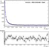 |
Fig. 1 Angular distribution of the PKS 2155-304 flare data set fitted with the H.E.S.S. point spread function (blue) from Monte Carlo simulations, resulting in a χ2/nd.o.f. = 91/72, with a P(χ2) of 0.06. The fit residuals are shown in the lower panel. |
2.2. Fermi-LAT analysis
The Fermi Gamma-ray Space Telescope, launched in 2008, observes the sky at energies between 20 MeV and 300 GeV (Atwood et al. 2009). The Fermi data analysis performed in this work used the LAT Science Tools package v9r23p1 (updated on 1st August 2011 to include the new PSFs) with the P7SOURCE_V6 post-launch instrument response function2. The standard event selection for a source well outside the galactic plane was applied. The analysis was performed for SOURCE event class photons. The analysis was further restricted to the energy range above 100 MeV, where the uncertainties in the effective area become smaller than 10%.
The data used for this analysis corresponds to more than 4 years of observations (4 August 2008–1 March 2013) for all three sources. To produce the spectra and flux upper limits, binnedAnalysis and UpperLimits Python modules were used, described in detail in the Fermi data analysis threads. As is the standard procedure, in order to take into account the broad Fermi PSF at low energies, all sources from the Second Fermi-LAT Catalog (2FGL, Nolan et al. 2012) within a 10-degree radius to the source position were included. The energy range of 100 MeV–300 GeV was split into logarithmically equal energy bins and in each bin a spectral analysis was performed, fixing the power law index of each source to be 2, and leaving the normalisation free. The normalisations for Galactic and extragalactic backgrounds were also left free in each energy bin. PKS 2155-304 and 1ES 1101-232 are detected in the dataset above an energy threshold of 100 MeV with significances of >100σ and 8.8σ, respectively. 1ES 0229+200 yields a TS value of 31.7 which corresponds to a significance of about 5.6σ. The recent results on 1ES 0229+200 presented by Vovk et al. (2012) are in agreement with the results presented in this paper.
The spectra of the sources can be well fitted with a single power law model with an index of Γ = 1.9 ± 0.2 for 1ES 1101-232, Γ = 1.5 ± 0.3 for 1ES 0229+200 and Γ = 1.85 ± 0.02 for PKS 2155-304, with only statistical errors given. These spectral indices are in good agreement with results from the 2FGL except for 1ES 0229+200, which was not listed in the catalogue.
3. Pair-halo constraints
Two separate techniques have been used to calculate pair halo (PH) upper limits from H.E.S.S. data: a model-dependent method and a model-independent method. With each method, upper limits for two different values of the photon index, 1.5 and 2.5, were calculated. These values were chosen to illustrate the expected range of indices of cascade emission at H.E.S.S. energies. A general model for the shape of cascade spectra was developed in Zdziarski (1988). A more recent model can be found in Eungwanichayapant & Aharonian (2009) and is depicted as the grey curve in Fig. 3. Although predictions at the high-energy end of the cascade strongly depend on the cut-off energy of the injection spectrum, an index of ~2 is expected in the energy range just before the secondary flux drops rapidly. The values 1.5 and 2.5 represent a broader range of possibilities. In addition, flux upper limits have been derived from Fermi-LAT data.
Model-dependent constraints
In the publication by Eungwanichayapant & Aharonian (2009), a study of the formation of PHs was conducted. In particular, the authors investigated the spectral and angular distributions of PHs in relation to the redshift of the central source, the spectral shape of the primary γ-rays, and the flux of the EBL. In the results used here from their study, the Primack et al. (2001) EBL model was adopted. In addition, the effects of the Franceschini et al. (2008) EBL model were investigated – these two models bound the present uncertainties in the EBL in the relevant wavelength range to some extent. Since the (1−10) μm EBL in the former model is ~40% larger than in the latter, the upper limits on a possible PH flux obtained with the Primack et al. (2001) EBL model are more conservative. On the other hand, recent independent studies of the EBL carried out by H.E.S.S. Collaboration (2013) suggest an EBL level between those motivated by the two EBL models considered.
For the Primack et al. (2001) EBL model, the differential angular distribution of a PH at z ≈ 0.13 and Eγ > 100 GeV, which best suits our data, was taken from Fig. 6 of Eungwanichayapant & Aharonian (2009) and is used here to derive limits on a possible PH flux. The effect of the slight differences between the assumed redshift in the model and the actual redshifts of the analysed sources is less than the effect of different EBL models and will therefore be neglected. The profile is based on calculations employing mono-energetic primary γ-rays with an energy E0 = 100 TeV. Provided the cut-off energy is high enough (>5 TeV), the differences in results for hard power-law and mono-energetic injection scenarios are minor (Aharonian et al. 2009a; Neronov et al. 2011). The resulting angular distribution follows a profile of dN/dθ ∝ θ−5/3. The angular distribution for the Franceschini et al. (2008) EBL model was generated by applying a scaling relation. Though such a simple relation is not sufficient to describe the effect of different EBL models on the angular shape of a PH in general, it is appropriate for the energies and redshifts discussed here (Eungwenichayapant & Aharonian, priv. comm., September 2013).
Pair halo flux upper limits for 1ES 1101-232, 1ES 0229+200, and PKS 2155-304 at a 99% C.L.
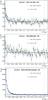 |
Fig. 2 Angular distribution of excess events of 1ES 1101-232 (top), 1ES 0229+200 (middle) and the PKS 2155-304 low state (bottom). The blue line is the H.E.S.S. PSF and the green line is the maximum allowed halo component. The model-independent limit on the pair-halo excess is calculated between the vertical dashed lines at 0.0125 deg2 and 0.02 deg2. |
Using these spatial models, “halo functions” were created for the measured θ2 distribution consisting of the PSF and the PH angular profiles, convolved with the PSF: N(θ2) = N(θ2)PSF + N(θ2)PH. The PSF normalisation was left free and the number of excess events in the PH model was increased until the fit had a probability <0.05. With this method, it was estimated how much of a halo component can be added to the overall shape without contradicting observations at a 99% confidence level (C.L.). In Fig. 2, the model-dependent analysis results are shown, under the assumption of the Primack et al. (2001) EBL model. For each of the three sources, the maximum possible halo component allowed by the observational data is depicted. As can be seen in the two upper panels of Fig. 2, due to low statistics, the total emission for both 1ES 1101-232 and 1ES 0229+200 can be fitted with the halo function. Therefore, the present angular profile data is unable to significantly constrain a PH component. In contrast, a strong constraint for a PH component of PKS 2155-304 could be derived. Relative to the central sources’ flux, which is about five times higher than the flux of 1ES 1101-232 and 1ES 0229+200, the upper limit on a pair halo around PKS 2155-304 is the lowest. This is clearly visible in the bottom panel of Fig. 2. For the lower EBL fluxes predicted by the Franceschini et al. (2008) model, the upper limits in the PKS 2155-304 case are even more constraining. Furthermore, although the flux’s upper limits presented in Table 3 seem high in comparison to the level of central point-like source fluxes, one has to keep in mind that the limits derived here apply to a comparatively large solid angle. The regions considered for the upper limit calculation are 2.1 × 10⁻⁴ sr (model-dependent) or 1.99 × 10⁻⁴ sr (model-independent), while more than 75% of the flux from a point source as seen by H.E.S.S. are detected in a region of 1.2 × 10⁻⁵ sr, marked at θ2 = 0.0125 deg2 in Fig. 2.
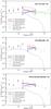 |
Fig. 3 Spectral energy distribution of 1ES 1101-232 (top), 1ES 0229+200 (middle), and PKS 2155-304 low state data sets (bottom). The H.E.S.S. data (green circles) and the Fermi data (empty circles) are shown. The upper limits on the flux contribution from a PH for the H.E.S.S. data are shown by blue and red arrows (dashed lines are model-dependent and solid lines are model-independent). The Fermi upper limits are shown as black squares. The grey line corresponds to the Halo Model taken from Eungwanichayapant & Aharonian (2009). |
To determine the differential flux limit, the maximum number of halo events was divided by the overall exposure, assuming a given photon index. This method was repeated for two different values of the photon index, 2.5 and 1.5. The resulting flux limits for both EBL models are listed in Table 3. The upper limits on the PH emission assuming the Primack et al. (2001) EBL model are shown in Fig. 3, together with the spectral energy distribution (SED) of the sources. The H.E.S.S. spectral data are previously published H.E.S.S. data taken from Aharonian et al. (2007c), Aharonian et al. (2007a), and Aharonian et al. (2009b), respectively. Model-dependent upper limits on the pair-halo flux are depicted for an assumed photon index of 2.5 and for an assumed index of 1.5.
Model-independent constraints.
In the model-independent approach, the residual emission after point source subtraction was used to derive an upper limit on the PH contribution. The expected contamination from the point-like source was calculated by taking the integral of the PSF in the region 0.0125 deg2 < θ2 < 0.2 deg2 (see Fig. 2), where the halo is expected to dominate the most. The lower limit is chosen according to the standard selection cut for point-like sources used by H.E.S.S. The Feldman Cousins Confidence Intervals (Feldman & Cousins 1998) were used to calculate the maximum halo excess at a 99% C.L. Similar to the model-dependent case, the differential limit was calculated by dividing the maximum possible number of halo events by the overall exposure, and the method was repeated for two different values of the photon index (Fig. 3). In several cases, unlike what is typically expected, the model-independent limits are more restricting than the model-dependent ones. This result is simply due to the poor statistics presently available for the 1 ES objects.
Constraints from Fermi-LAT data
Since the pair halo is expected to be a diffuse source for Fermi, a spatial model (∝θ−5/3) based on theoretical estimations of the halo angular profile (Eungwanichayapant & Aharonian 2009) was used. The binned Fermi analysis was performed at energies 300 MeV–300 GeV for the models with and without a halo component. In all considered cases, the models with a halo have similar log-likelihood values to the models without the halo contribution, thus no significant indications for pair-halo emission are found. The upper limits on the fluxes at a 99% C.L. were calculated with the UpperLimits Python module of the Fermi software and are shown in Fig. 3.
4. Magnetically broadened cascade constraints
In this section a model-dependent approach was applied in order to investigate whether evidence is found for a MBC in the angular event distribution of blazar fluxes observed with H.E.S.S. A 3D Monte-Carlo description of MBCs developed in Taylor et al. (2011) was utilised here to determine the expected angular profile of this emission for different EGMF strengths. For these calculations, both the Franceschini et al. (2008) and the Primack et al. (2001) EBL models were used. Using this description, the range of EGMF values excluded by the present H.E.S.S. results was investigated. A method similar to the model-dependent approach described in Sect. 3 was used to obtain these constraints: a spatial MBC model function N(θ2) = N(θ2)PSF + N(θ2)MBC was created, N(θ2)MBC being the MBC model from simulations convolved with the H.E.S.S. PSF. In the same manner as for the model-dependent PH limits, the PSF normalisation was left free and the number of MBC events was increased until it contradicted the observational results at a 99% C.L. The ratio of maximum allowed MBC events was then compared to the ratios predicted by the Monte-Carlo simulations for different magnetic field strengths. In the simulations, photon indices of 1.9, 1.5, and 1.9 for 1ES 1101-232, 1ES 0229+200, and PKS 2155-304, respectively, were motivated from the Fermi analysis of their GeV spectra. The spectra of all three of the blazars used in this study are consistent with a power-law spectrum with a cut-off at multi-TeV energies. Therefore, for each of the sources an injection spectrum of the form dN/dE ∝ E−Γe−E/Emax with a cut-off Emax = 10 TeV was adopted to ensure that a sufficient amount of the cascade component lies in the H.E.S.S. energy range (see Eungwanichayapant & Aharonian 2009).
For the MBC scenario, both the observed SED and angular spread of the arriving flux depend significantly on the EGMF. The angular spreading effect is seen explicitly in Fig. 4, for which the effect of 10-14 G, 10-15 G, and 10-16 G EGMF values are considered. A 1 Mpc coherence length is adopted as a fiducial value, although higher values have been discussed recently (Durrer & Neronov 2013). Essentially, the effect of the coherence length can be neglected if it is more than the cooling length of the multi-TeV cascade electrons of relevance here. In contrast, the choice of the EBL model plays an important role. Again, the Primack et al. (2001) EBL model is expected to result in more conservative bounds on the maximum cascade contribution since it is about 40% higher than the Franceschini et al. (2008) EBL model at the wavelengths of interest here.
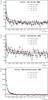 |
Fig. 4 Angular distribution of excess events of 1ES 1101-232 (top), 1ES 0229+200 (middle) and the PKS 2155-304 low state (bottom). The H.E.S.S. data (black points) are plotted against the angular distribution of the MBC model for varying magnetic field strengths. The red, violet, and cyan lines correspond to the maximum cascade flux for magnetic field strengths of 10-14, 10-15 and 10-16 G, simulated under the assumption of the Franceschini et al. (2008) EBL model. |
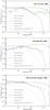 |
Fig. 5 1ES 1101-232 (top), 1ES 0229+200 (middle) and PKS 2155-304 (bottom) spectral energy distributions (Γ = 1.9, 1.5, and 1.9 respectively), including Fermi data (empty blue circles) and the H.E.S.S. results (solid green circles). The dotted grey line shows the expected cascade SED assuming the EGMF strength is 0 G, and the solid grey line shows this component added to the attenuated direct emission SED (dashed red line). |
In Fig. 4, the angular profiles of the MBCs resulting from calculations with the Franceschini et al. (2008) model are shown. Though the comparably low statistics for both 1ES 1101-232 and 1ES 0229+200 limit any constraint from their measured angular profiles, a strong constraint is provided by the angular profile of PKS 2155-304. For this object, a mild cascade contribution was found to be expected in the arriving VHE photon flux. As can be seen in Fig. 6, for PKS 2155-304 the maximum ratio of MBC events in the H.E.S.S. data conflicts with the expected ratio of cascade photons introduced by field strengths of ~10-15 G or a factor of a few stronger. Assuming the Primack et al. (2001) EBL model, the range of excluded EGMF strengths is (0.3−10) × 10-15 G. On the other hand, the Franceschini et al. (2008) EBL model is the conservative choice when excluding EGMF strengths. Since it predicts a much lower cascade fraction for B = 10-14 G, such a magnetic field strength regime can not be ruled out when assuming this EBL model. For stronger fields the cascade contribution’s fraction to the overall arriving flux, relative to that of the direct emission component, reduces significantly due to isotropisation. Consequently, the subsequent angular spreading for higher EGMF values becomes indistinguishable from the H.E.S.S. PSF. Thus, for EGMF values, such as those present in the PH scenario discussed in Sect. 3, the angular profiles can be significantly smaller than those found for the case of a 10-15 G EGMF value. This strong EGMF suppression effect explains why the above derived 99% C.L. on the EGMF value constrains only a decade of the EGMF range. In addition, all bounds depend on whether the intrinsic cut-off energy is high enough. For the two EBL models considered, Primack et al. (2001) and Franceschini et al. (2008), a minimum cut-off above 3 TeV is required such that some constraint is obtainable. For a higher cut-off energy than the value adopted in this study, the range of excluded EGMF would be a few times larger.
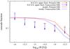 |
Fig. 6 EGMF constraints on PKS 2155-304. The dashed blue line depicts the expected fraction of MBC events in the VHE data depending on the EGMF strength, assuming the Franceschini et al. (2008) EBL model. Blue arrows are the maximum fractions of MBC events for the EBL model not to contradict the angular profile data of PKS 2155-304 at a 99% C.L. The expected cascade fraction and the corresponding upper limit from H.E.S.S. data under the assumption of the Primack et al. (2001) EBL model are depicted in red. |
5. Discussion and conclusions
The search for a pair-halo component in the H.E.S.S. and Fermi-LAT data from regions surrounding the VHE γ-ray sources 1ES 1101-232, 1ES 0229+200, and PKS 2155-304 shows no indication of such emission. From our analysis, flux upper limits on the extended VHE γ-ray emission from the three sources analysed have been found to be at the level of a few percentage points of the Crab nebula flux. For example, the model-independent upper limits on the pair-halo flux for an assumed photon index of 2.5 are <2%, <3%, and <8% of the integrated Crab nebula flux above 1 TeV3 for 1ES 1101-23, 1ES 0229+200, and PKS 2155-304, respectively, adopting the Primack et al. (2001) EBL model. Also with the analyses of Fermi-LAT data, no significant pair-halo emission was detected and energy-binned flux upper limits for a θ−5/3 profile were calculated. Though these limits are comparable to previously obtained values by other instruments for other blazars, the detailed angular modelling from recent theoretical work on the topic, adopted by this study, marks a significant improvement over previous limits. While the most constraining upper limit values in Aharonian et al. (2001), Aleksić et al. (2010), and Ackermann et al. (2013) were derived by varying the angular size of the extended emission model, the analysis at hand gives all limits with a physically motivated fixed size. However, with the method presented here, upper limits would become more constraining the less the expected extended emission is similar to the PSF. The constraints obtained from this pair-halo analysis can be used to set limits on the γ-ray output from these AGN over the past ~105 years. If any of these AGN had been more active in the past, more pairs would have been subsequently produced. Consequently, for sufficiently strong EGMF values (>10-12 G), increased activity in the past would strengthen the constraint on the extended emission component. Since the EGMF strength required for the pair-halo scenario leads to the isotropisation of the cascade emission, the observed luminosity of this secondary component may be significantly reduced compared to the apparent luminosity of the primary beamed component. Not detecting the secondary component, therefore, means we are unable to place constraints on the EGMF strength.
The limits of the PH γ-ray energy flux for the three blazars may be
converted into limits on the accumulated electron energy density in the surrounding regions.
As an example case, 1ES 0229+200 is considered, whose energy flux at 0.5 TeV is
~10-12 erg cm-2 s-1. Assuming that the corresponding
photons result from a pair-halo cascade with strong EGMF (>10-12 G), the parent ~15 TeV electrons and positrons will both be
born into and isotropised within a region ~10 Mpc
from the blazar. For this strong field case, an upper limit on the TeV γ-ray luminosity from these
regions is ~4 × 1042 erg s-1. Since the electron IC cooling
time on the CMB is  105 yr, a limit on the total energy content of the parent
electrons is ~1055 erg.
105 yr, a limit on the total energy content of the parent
electrons is ~1055 erg.
A search for MBC emission in the arriving flux from the three blazars was also carried out.
The datasets for both 1ES 1101-232 and 1ES 0229+200 are found not to be statistically
constraining at present. However, a constraint was found to be obtainable using the PKS
2155-304 observational results. From H.E.S.S. observations of the angular profile for PKS
2155-304, EGMF values were excluded for the range (0.3−3) × 10-15 G (for a coherence length of
1 Mpc), at the 99% C.L. This
range is excluded for both EBL models adopted here, the Primack et al. (2001) and the Franceschini et al.
(2008) model. For a coherence length scale λB shorter than the cascade
electron cooling lengths, the lower EGMF limit scales as
 , as demonstrated in Neronov et al. (2013). Conversely, for λB longer than these
cooling lengths, the constraint is independent of λB. As shown in Fig. 6,
stronger magnetic fields than the upper limit result in the cascade component dropping below
the direct emission contribution, reducing the overall angular width below the H.E.S.S.
resolution limits.
, as demonstrated in Neronov et al. (2013). Conversely, for λB longer than these
cooling lengths, the constraint is independent of λB. As shown in Fig. 6,
stronger magnetic fields than the upper limit result in the cascade component dropping below
the direct emission contribution, reducing the overall angular width below the H.E.S.S.
resolution limits.
Furthermore, our bound on the EGMF is compatible with the analytic estimates put forward in Aleksić et al. (2010), although the analysis presented here is the most robust to date due to the theoretical modelling that has been employed.
Interestingly, the success proven by this method demonstrates its complementarity as an EGMF probe in light of the multi-wavelength SED method employed in previous studies (Neronov & Vovk 2010; Dolag et al. 2011; Tavecchio et al. 2011; and Taylor et al. 2011). These studies probed EGMF values for which no notable angular broadening would be expected. Instead, the effect of the EGMF was to introduce energy-dependent time delays on the arriving cascade. Ensuring that the source variability timescale sits at a level compatible with what is currently observed, i.e. the sources are steady on 3 yr timescales, placed a constraint on the EGMF at a level of >10-17 G (Taylor et al. 2011; Dermer et al. 2011). In contrast to this time delay SED method, our angular profile investigations are insensitive to the source variability timescale. In this way, the constraints provided by the angular profile studies of blazars offer a complementary new probe into the EGMF that allows field strengths with values > 10-15 G to be investigated.
The future prospects for observing both extended halo emission and MBCs are promising. In the near future, H.E.S.S. phase-II offers great potential with its ability to detect γ-rays in the energy band between Fermi-LAT and H.E.S.S. phase-I. In the longer term, the Cherenkov Telescope Array (CTA; see e.g. CTA Consortium et al. 2013), with a larger array size, a wider field of view, improved angular resolution along with greater sensitivity, will allow for a deeper probing of these elusive phenomena.
See http://tevcat.uchicago.edu for an up-to-date list.
See http://fermi.gsfc.nasa.gov/ssc/data/ for public Fermi data and analysis software.
(2.26 ± 0.03) × 10-11 cm-1 s-1, see Aharonian et al. (2006).
Acknowledgments
The support of the Namibian authorities and of the University of Namibia in facilitating the construction and operation of H.E.S.S. is gratefully acknowledged, as is the support by the German Ministry for Education and Research (BMBF), the Max Planck Society, the German Research Foundation (DFG), the French Ministry for Research, the CNRS-IN2P3 and the Astroparticle Interdisciplinary Programme of the CNRS, the UK Science and Technology Facilities Council (STFC), the IPNP of the Charles University, the Czech Science Foundation, the Polish Ministry of Science and Higher Education, the South African Department of Science and Technology and National Research Foundation, and by the University of Namibia. We appreciate the excellent work of the technical support staff in Berlin, Durham, Hamburg, Heidelberg, Palaiseau, Paris, Saclay, and in Namibia in the construction and operation of the equipment. The authors are grateful to the referee who helped to considerably improve the quality of the paper.
References
- Abramowski, A., Acero, F., & Aharonian, F., et al. (H.E.S.S. Collaboration) 2013, A&A, 550, A4 [NASA ADS] [CrossRef] [EDP Sciences] [Google Scholar]
- Acharya, B. S., Actis, M., Aghajani, T., et al. (CTA Consortium) 2013, Astropart. Phys., 43, 3 [Google Scholar]
- Ackermann, M., Ajello, M., Allafort, A., et al. (Fermi-LAT Collaboration) 2013, ApJ, 765, 54 [NASA ADS] [CrossRef] [Google Scholar]
- Aharonian, F., Akhperjanian, A. G., Aye, K., et al. (H.E.S.S. Collaboration) 2004, Astropart. Phys., 22, 109 [NASA ADS] [CrossRef] [Google Scholar]
- Aharonian, F., Akhperjanian, A. G., Aye, K., et al. (H.E.S.S. Collaboration) 2005, A&A, 430, 865 [NASA ADS] [CrossRef] [EDP Sciences] [Google Scholar]
- Aharonian, F., Akhperjanian, A. G., Bazer-Bachi, A. R., et al. (H.E.S.S. Collaboration) 2006, A&A, 457, 899 [NASA ADS] [CrossRef] [EDP Sciences] [Google Scholar]
- Aharonian, F., Akhperjanian, A. G., Barres de Almeida, U., et al. (H.E.S.S. Collaboration) 2007a, A&A, 475, L9 [NASA ADS] [CrossRef] [EDP Sciences] [Google Scholar]
- Aharonian, F., Akhperjanian, A. G., Bazer-Bachi, A. R., et al. (H.E.S.S. Collaboration) 2007b, ApJ, 664, L71 [Google Scholar]
- Aharonian, F., Akhperjanian, A. G., Bazer-Bachi, A. R., et al. (H.E.S.S. Collaboration) 2007c, A&A, 470, 475 [NASA ADS] [CrossRef] [EDP Sciences] [Google Scholar]
- Aharonian, F., Akhperjanian, A. G., Anton, G., et al. (H.E.S.S. Collaboration) 2009a, A&A, 502, 749 [NASA ADS] [CrossRef] [EDP Sciences] [Google Scholar]
- Aharonian, F., Akhperjanian, A. G., Anton, G., et al. (H.E.S.S. Collaboration) 2009b, ApJ, 696, L150 [NASA ADS] [CrossRef] [Google Scholar]
- Aharonian, F. A., Coppi, P. S., & Voelk, H. J. 1994, ApJ, 423, L5 [NASA ADS] [CrossRef] [Google Scholar]
- Aharonian, F. A., Akhperjanian, A. G., Barrio, J. A., et al. (H.E.S.S. Collaboration) 2001, A&A, 366, 746 [NASA ADS] [CrossRef] [EDP Sciences] [Google Scholar]
- Aharonian, F. A., Timokhin, A. N., & Plyasheshnikov, A. V. 2002, A&A, 384, 834 [NASA ADS] [CrossRef] [EDP Sciences] [Google Scholar]
- Aleksić, J., Antonelli, L. A., Antoranz, P., et al. 2010, A&A, 524, A77 [NASA ADS] [CrossRef] [EDP Sciences] [Google Scholar]
- Ando, S., & Kusenko, A. 2010, ApJ, 722, L39 [NASA ADS] [CrossRef] [Google Scholar]
- Arlen, T. C., Vassiliev, V. V., Weisgarber, T., Wakely, S. P., & Yusef Shafi, S. 2012 [arXiv:1210.2802] [Google Scholar]
- Atwood, W. B., Abdo, A. A., Ackermann, M., et al. 2009, ApJ, 697, 1071 [NASA ADS] [CrossRef] [Google Scholar]
- Benbow, W. 2005, Proc. Conf. Towards a Network of Atmospheric Cherenkov Detectors VII (Palaiseau, France: Ecole Polytechnique), 163 [Google Scholar]
- Broderick, A. E., Chang, P., & Pfrommer, C. 2012, ApJ, 752, 22 [NASA ADS] [CrossRef] [Google Scholar]
- Chadwick, P. M., Lyons, K., McComb, T. J. L., et al. 1999, ApJ, 513, 161 [NASA ADS] [CrossRef] [Google Scholar]
- de Naurois, M., & Rolland, L. 2009, Astropart. Phys., 32, 231 [NASA ADS] [CrossRef] [Google Scholar]
- Dermer, C. D., Cavadini, M., Razzaque, S., et al. 2011, ApJ, 733, L21 [NASA ADS] [CrossRef] [Google Scholar]
- Dolag, K., Kachelriess, M., Ostapchenko, S., & Tomàs, R. 2011, ApJ, 727, L4 [NASA ADS] [CrossRef] [Google Scholar]
- Durrer, R., & Neronov, A. 2013, A&AR, 21, 62 [Google Scholar]
- Essey, W., Kalashev, O., Kusenko, A., & Beacom, J. F. 2011, ApJ, 731, 51 [NASA ADS] [CrossRef] [Google Scholar]
- Eungwanichayapant, A., & Aharonian, F. 2009, Int. J. Mod. Phys. D, 18, 911 [NASA ADS] [CrossRef] [Google Scholar]
- Falomo, R., Scarpa, R., & Bersanelli, M. 1994, ApJS, 93, 125 [NASA ADS] [CrossRef] [Google Scholar]
- Feldman, G. J., & Cousins, R. D. 1998, Phys. Rev. D, 57, 3873 [Google Scholar]
- Franceschini, A., Rodighiero, G., & Vaccari, M. 2008, A&A, 487, 837 [NASA ADS] [CrossRef] [EDP Sciences] [Google Scholar]
- Gould, R. J., & Rephaeli, Y. 1978, ApJ, 225, 318 [NASA ADS] [CrossRef] [Google Scholar]
- Gould, R. J., & Schréder, G. 1966, Phys. Rev. Lett., 16, 252 [Google Scholar]
- Hinton, J. A. 2004, New Astron. Rev., 48, 331 [NASA ADS] [CrossRef] [Google Scholar]
- Jelley, J. V. 1966, Phys. Rev. Lett., 16, 479 [NASA ADS] [CrossRef] [Google Scholar]
- Li, T., & Ma, Y. 1983, ApJ, 272, 317 [NASA ADS] [CrossRef] [Google Scholar]
- Lind, K. R., & Blandford, R. D. 1985, ApJ, 295, 358 [NASA ADS] [CrossRef] [Google Scholar]
- Meyer, M., Raue, M., Mazin, D., & Horns, D. 2012, A&A, 542, A59 [NASA ADS] [CrossRef] [EDP Sciences] [Google Scholar]
- Miniati, F., & Bell, A. 2011, ApJ, 729, 73 [NASA ADS] [CrossRef] [Google Scholar]
- Miniati, F., & Elyiv, A. 2013, ApJ, 770, 54 [NASA ADS] [CrossRef] [Google Scholar]
- Neronov, A., & Semikoz, D. V. 2009, Phys. Rev. D, 80, 123012 [NASA ADS] [CrossRef] [Google Scholar]
- Neronov, A., & Vovk, I. 2010, Science, 328, 73 [NASA ADS] [CrossRef] [PubMed] [Google Scholar]
- Neronov, A., Semikoz, D. V., Tinyakov, P. G., & Tkachev, I. I. 2011, A&A, 526, A90 [NASA ADS] [CrossRef] [EDP Sciences] [Google Scholar]
- Neronov, A., Taylor, A. M., Tchernin, C., & Vovk, I. 2013, A&A, 554, A31 [NASA ADS] [CrossRef] [EDP Sciences] [Google Scholar]
- Nikishov, A. I. 1962, Sov. Phys. JETP, 14, 393 [Google Scholar]
- Nolan, P. L., Abdo, A. A., Ackermann, M., et al. 2012, ApJS, 199, 31 [NASA ADS] [CrossRef] [Google Scholar]
- Primack, J. R., Somerville, R. S., Bullock, J. S., & Devriendt, J. E. G. 2001, in AIP Conf. Ser. 558, eds. F. A. Aharonian, & H. J. Völk, 463 [Google Scholar]
- Schlickeiser, R., Ibscher, D., & Supsar, M. 2012, ApJ, 758, 102 [NASA ADS] [CrossRef] [Google Scholar]
- Stecker, F. W., & de Jager, O. C. 1993, ApJ, 415, L71 [NASA ADS] [CrossRef] [Google Scholar]
- Tavecchio, F., Ghisellini, G., Foschini, L., et al. 2010, MNRAS, 406, L70 [NASA ADS] [Google Scholar]
- Tavecchio, F., Ghisellini, G., Bonnoli, G., & Foschini, L. 2011, MNRAS, 414, 3566 [NASA ADS] [CrossRef] [Google Scholar]
- Taylor, A. M., Vovk, I., & Neronov, A. 2011, A&A, 529, A144 [NASA ADS] [CrossRef] [EDP Sciences] [Google Scholar]
- Vovk, I., Taylor, A. M., Semikoz, D., & Neronov, A. 2012, ApJ, 747, L14 [NASA ADS] [CrossRef] [Google Scholar]
- Woo, J., Urry, C. M., van der Marel, R. P., Lira, P., & Maza, J. 2005, ApJ, 631, 762 [NASA ADS] [CrossRef] [Google Scholar]
- Zdziarski, A. A. 1988, ApJ, 335, 786 [NASA ADS] [CrossRef] [Google Scholar]
All Tables
Summary of the H.E.S.S. analysis results for 1ES 1101-232, 1ES 0229+200 and PKS 2155-304.
Pair halo flux upper limits for 1ES 1101-232, 1ES 0229+200, and PKS 2155-304 at a 99% C.L.
All Figures
|
Fig. 1 Angular distribution of the PKS 2155-304 flare data set fitted with the H.E.S.S. point spread function (blue) from Monte Carlo simulations, resulting in a χ2/nd.o.f. = 91/72, with a P(χ2) of 0.06. The fit residuals are shown in the lower panel. |
| In the text | |
|
Fig. 2 Angular distribution of excess events of 1ES 1101-232 (top), 1ES 0229+200 (middle) and the PKS 2155-304 low state (bottom). The blue line is the H.E.S.S. PSF and the green line is the maximum allowed halo component. The model-independent limit on the pair-halo excess is calculated between the vertical dashed lines at 0.0125 deg2 and 0.02 deg2. |
| In the text | |
|
Fig. 3 Spectral energy distribution of 1ES 1101-232 (top), 1ES 0229+200 (middle), and PKS 2155-304 low state data sets (bottom). The H.E.S.S. data (green circles) and the Fermi data (empty circles) are shown. The upper limits on the flux contribution from a PH for the H.E.S.S. data are shown by blue and red arrows (dashed lines are model-dependent and solid lines are model-independent). The Fermi upper limits are shown as black squares. The grey line corresponds to the Halo Model taken from Eungwanichayapant & Aharonian (2009). |
| In the text | |
|
Fig. 4 Angular distribution of excess events of 1ES 1101-232 (top), 1ES 0229+200 (middle) and the PKS 2155-304 low state (bottom). The H.E.S.S. data (black points) are plotted against the angular distribution of the MBC model for varying magnetic field strengths. The red, violet, and cyan lines correspond to the maximum cascade flux for magnetic field strengths of 10-14, 10-15 and 10-16 G, simulated under the assumption of the Franceschini et al. (2008) EBL model. |
| In the text | |
|
Fig. 5 1ES 1101-232 (top), 1ES 0229+200 (middle) and PKS 2155-304 (bottom) spectral energy distributions (Γ = 1.9, 1.5, and 1.9 respectively), including Fermi data (empty blue circles) and the H.E.S.S. results (solid green circles). The dotted grey line shows the expected cascade SED assuming the EGMF strength is 0 G, and the solid grey line shows this component added to the attenuated direct emission SED (dashed red line). |
| In the text | |
|
Fig. 6 EGMF constraints on PKS 2155-304. The dashed blue line depicts the expected fraction of MBC events in the VHE data depending on the EGMF strength, assuming the Franceschini et al. (2008) EBL model. Blue arrows are the maximum fractions of MBC events for the EBL model not to contradict the angular profile data of PKS 2155-304 at a 99% C.L. The expected cascade fraction and the corresponding upper limit from H.E.S.S. data under the assumption of the Primack et al. (2001) EBL model are depicted in red. |
| In the text | |
Current usage metrics show cumulative count of Article Views (full-text article views including HTML views, PDF and ePub downloads, according to the available data) and Abstracts Views on Vision4Press platform.
Data correspond to usage on the plateform after 2015. The current usage metrics is available 48-96 hours after online publication and is updated daily on week days.
Initial download of the metrics may take a while.