© ESO, 2014

1. Introduction

Quiescent solar prominences are usually thought to be cool (T ≈ 10⁴ K) and dense (ρ ≈ 10^-12−10^-10 kg m^-3) plasma clouds located in less dense and hotter solar corona. It is still a matter of debate how these dense and cool structures live for a long time within the solar corona, although a widely extended idea is that their support and thermal isolation are of magnetic origin. They form along the inversion polarity line, or between the weak remnants of active regions. Prominences are highly dynamic structures subject to small amplitude oscillations, which have been routinely observed from the ground and from space, and the details about their properties can be found in Oliver & Ballester (2002); Banerjee et al. (2007); Oliver (2009); Mackay et al. (2010); and Arregui & Ballester (2011). See also Arregui et al. (2012) for a comprehensive review of solar prominence oscillations. These small amplitude oscillations are characterized by one or more of the following features: they are not related to flare activity; they display small amplitude velocities and are of local nature, where only some regions of the prominence display periodic motions. The most common technique to study prominence oscillations is to place a spectrograph slit on a prominence and to record one or more spectral lines along a time interval. The analysis of the obtained data provides the time series of several indicators such as Doppler velocity, line width, and line intensity, whose time behavior can be analyzed. Tsubaki (1988) and Oliver (1999) pointed out that in most of the papers devoted to observations of prominence oscillations, the periodicity is usually found in only one of the above mentioned spectral indicators. For instance, Landman et al. (1977) observed periodic fluctuations in the line intensity and width with period around 22 min but not in the Doppler shift. Yi et al. (1991) detected periods of 5 and 12 min in the power spectra of the line-of-sight velocity and the line intensity. Also, Suematsu et al. (1990) found signs of a ~60 min periodic variation in the Doppler velocity, line intensity, and line width. However, the Doppler signal also displayed shorter period variations (with periods around 4 and 14 min), which were not present in the other two data sets. This observation points out a striking feature already found in other investigations, namely that the temporal behavior of various indicators corresponding to the same time series of spectra is not the same because either they show different periods in their power spectra (Tsubaki et al. 1987) or one indicator presents a clear periodicity, while the others do not (Wiehr et al. 1984; Tsubaki & Takeuchi 1986; Balthasar et al. 1986; Tsubaki et al. 1988; Suetterlin et al. 1997). Finally, Balthasar & Wiehr (1994) simultaneously observed the spectral lines He i 3888 Å, H₈ 3889 Å  and Ca ii 8498 Å. From this information, they analyzed the temporal variations in the thermal and non-thermal line broadenings, the total H₈ line intensity, the He i 3888 Å to H₈ emission ratio, and the Doppler shift of the three spectral lines, which correlated well and thus reduced to a single data set. The power spectra of all these parameters yield a large number of power maxima, but only two of them (with periods of 29 and 78 min) are present in more than one indicator.

The interpretation of the observational results summarized above appears to be difficult. These oscillations have been commonly interpreted in terms of standing or propagating magnetohydrodynamic (MHD) waves, and using this interpretation, a number of theoretical models have been set up to try to understand the prominence oscillatory behavior. Theoretical models can provide the temporal behavior of the plasma velocity, temperature, density, and other physical parameters, while observations yield information on quantities such as the line intensity or the line width and shift (line asymmetry). Therefore, a clear identification of the spectral parameters with density, pressure, temperature, etc. is required before any progress can be achieved. Then, the presence of a certain period in more than one signal could be used to infer the properties of the MHD mode involved. Another source of useful information could be the detection of a given period in one signal but not in the others, as discussed above.

Taking into account the above considerations, our main aim here is to explore the relationship between spectral indicators, such as Doppler shift, line intensity, and line half-width and the linear perturbations induced in a simple prominence model. The layout of the paper is as follows: in Sect. 2, the equilibrium model and some theoretical considerations are presented; in Sect. 3, we describe the method of solving the radiative-transfer problem in oscillatory prominences; Sect. 4 contains our numerical results and their analysis. Finally, our conclusions are drawn in Sect. 5.

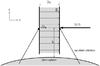Fig. 1 Sketch of the geometry of the considered problem common for the MHD simulation and for the radiative transfer. The prominence slab with infinite height and length and width 2x0 is penetrated by a constant magnetic field. For a radiative transfer, we should take into account incident radiation from the surface (dashed arrows), according to the position above the solar limb (h). The line-of-sight is perpendicular to the slab.

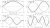Fig. 2 Velocity perturbations along the x-axis of the slab for the fundamental slow mode (fS, top left), the first slow overtone (1S, top right), the fundamental fast mode (fF, bottom left) and the first fast overtone (1F, bottom right). The x-axes of plots are scaled in meters. Note the different velocity scale. Different lines represent different phases (i.e. time divided by period), as labelled at the top left corner of each plot. For phase =0.25 and phase =0.75, the lines are merged. Oscillatory periods are shown at the top right corner of each plot.

2. Model and methods

For our equilibrium configuration, we use a homogeneous slab bounded in the transverse direction with a width 2x₀ but of infinite length in the direction along the slab, as well as infinite height (see Fig. 1). Such a slab is threaded by a constant transverse magnetic field, which we assume to be anchored in the lateral walls of the slab. The equilibrium magnitudes of the slab are given by: 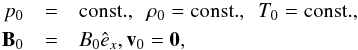$\begin{array}{ccc}{\mathit{p}}_{\mathrm{0}}& \mathrm{=}& \mathrm{const}\mathit{.}\mathit{,}{\mathit{\rho }}_{\mathrm{0}}\mathrm{=}\mathrm{const}\mathit{.}\mathit{,}{\mathit{T}}_{\mathrm{0}}\mathrm{=}\mathrm{const}\mathit{.}\mathit{,}\\ {{B}}_{\mathrm{0}}& \mathrm{=}& {\mathit{B}}_{\mathrm{0}}\mathit{ê}\mathit{x}\mathit{,}{{v}}_{\mathrm{0}}\mathrm{=}{0}\mathit{,}\end{array}$with B₀ = 5 × 10^-4 T; ρ₀ = 2.41 × 10^-10 kg m^-3; $\frac{{\mathit{T}}_{\mathrm{0}}}{\begin{array}{c}{}_{\mathrm{˜}}\\ \mathit{\mu }\end{array}}\mathrm{=}{\mathrm{10}}^{\mathrm{4}}$ K; p₀ = 0.02 Pa, and x₀ = 6 × 10⁶ m. Moreover, $\begin{array}{c}{}_{\mathrm{˜}}\\ \mathit{\mu }\end{array}\mathrm{=}\mathrm{0.6}$ for fully ionized plasma, which means that T₀ = 6000 K. With these parameters, the sound speed is: 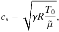$\begin{array}{ccc}{\mathit{c}}_{\mathrm{s}}\mathrm{=}\sqrt{\mathit{\gamma R}\frac{{\mathit{T}}_{\mathrm{0}}}{\begin{array}{c}\mathrm{˜}\\ \mathit{\mu }\end{array}}}\mathit{,}& & \end{array}$where c_s = 11761.5 m s^-1 and the Alfvén speed is 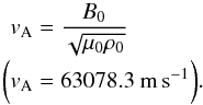$\begin{array}{ccc}{\mathit{v}}_{\mathrm{A}}& \mathrm{=}& \frac{{\mathit{B}}_{\mathrm{0}}}{\sqrt{{\mathit{\mu }}_{\mathrm{0}}{\mathit{\rho }}_{\mathrm{0}}}}\\ ({\mathit{v}}_{\mathrm{A}}& \mathrm{=}& \mathrm{63078.3}\mathrm{m}\hspace{0.17em}{\mathrm{s}}^{-1})\mathit{.}\end{array}$We consider linear and adiabatic MHD waves with small perturbations from the equilibrium in the form:

$\begin{array}{ccc}& & {B}\mathrm{\left(}\mathit{t,}{r}\mathrm{\right)}\mathrm{=}{{B}}_{\mathrm{0}}\mathrm{+}{{B}}_{\mathrm{1}}\mathrm{\left(}\mathit{t,}{r}\mathrm{\right)}\mathit{,}\\ & & \mathit{p}\mathrm{\left(}\mathit{t,}{r}\mathrm{\right)}\mathrm{=}{\mathit{p}}_{\mathrm{0}}\mathrm{+}{\mathit{p}}_{\mathrm{1}}\mathrm{\left(}\mathit{t,}{r}\mathrm{\right)}\mathit{,\rho }\mathrm{\left(}\mathit{t,}{r}\mathrm{\right)}\mathrm{=}{\mathit{\rho }}_{\mathrm{0}}\mathrm{+}{\mathit{\rho }}_{\mathrm{1}}\mathrm{\left(}\mathit{t,}{r}\mathrm{\right)}\mathit{,}\\ & & \mathit{T}\mathrm{\left(}\mathit{t,}{r}\mathrm{\right)}\mathrm{=}{\mathit{T}}_{\mathrm{0}}\mathrm{+}{\mathit{T}}_{\mathrm{1}}\mathrm{\left(}\mathit{t,}{r}\mathrm{\right)}\mathit{,}{v}\mathrm{\left(}\mathit{t,}{r}\mathrm{\right)}\mathrm{=}{{v}}_{\mathrm{1}}\mathrm{\left(}\mathit{t,}{r}\mathrm{\right)}\mathit{.}\end{array}$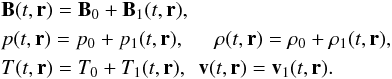In addition, all perturbed variables, f₁(t,r), are taken as: 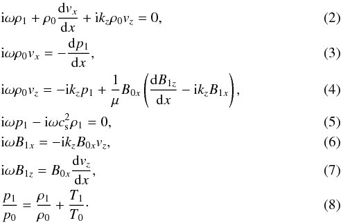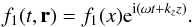${\mathit{f}}_{\mathrm{1}}\mathrm{\left(}\mathit{t,}{r}\mathrm{\right)}\mathrm{=}{\mathit{f}}_{\mathrm{1}}\mathrm{\left(}\mathit{x}\mathrm{\right)}{\mathrm{e}}^{\mathrm{i}\left(\mathit{\omega t}\mathrm{+}{\mathit{k}}_{\mathit{z}}\mathit{z}\right)}\mathit{.}$(1)This corresponds to waves that propagate in the z-direction along the prominence slab. Considering only motions in the xz-plane, the linearized MHD equations reduce to:

$\begin{array}{ccc}& & \mathrm{i}\mathit{\omega }{\mathit{\rho }}_{\mathrm{1}}\mathrm{+}{\mathit{\rho }}_{\mathrm{0}}\frac{\mathrm{d}{\mathit{v}}_{\mathit{x}}}{\mathrm{d}\mathit{x}}\mathrm{+}\mathrm{i}{\mathit{k}}_{\mathit{z}}{\mathit{\rho }}_{\mathrm{0}}{\mathit{v}}_{\mathit{z}}\mathrm{=}\mathrm{0}\mathit{,}\\ & & \mathrm{i}\mathit{\omega }{\mathit{\rho }}_{\mathrm{0}}{\mathit{v}}_{\mathit{x}}\mathrm{=}\mathrm{-}\frac{\mathrm{d}{\mathit{p}}_{\mathrm{1}}}{\mathrm{d}\mathit{x}}\mathit{,}\\ & & \mathrm{i}\mathit{\omega }{\mathit{\rho }}_{\mathrm{0}}{\mathit{v}}_{\mathit{z}}\mathrm{=}\mathrm{-}\mathrm{i}{\mathit{k}}_{\mathit{z}}{\mathit{p}}_{\mathrm{1}}\mathrm{+}\frac{\mathrm{1}}{\mathit{\mu }}{\mathit{B}}_{\mathrm{0}\mathit{x}}\left(\frac{\mathrm{d}{\mathit{B}}_{\mathrm{1}\mathit{z}}}{\mathrm{d}\mathit{x}}\mathrm{-}\mathrm{i}{\mathit{k}}_{\mathit{z}}{\mathit{B}}_{\mathrm{1}\mathit{x}}\right)\mathit{,}\\ & & \mathrm{i}\mathit{\omega }{\mathit{p}}_{\mathrm{1}}\mathrm{-}\mathrm{i}\mathit{\omega }{\mathit{c}}_{\mathrm{s}}^{\mathrm{2}}{\mathit{\rho }}_{\mathrm{1}}\mathrm{=}\mathrm{0}\mathit{,}\\ & & \mathrm{i}\mathit{\omega }{\mathit{B}}_{\mathrm{1}\mathit{x}}\mathrm{=}\mathrm{-}\mathrm{i}{\mathit{k}}_{\mathit{z}}{\mathit{B}}_{\mathrm{0}\mathit{x}}{\mathit{v}}_{\mathit{z}}\mathit{,}\\ & & \mathrm{i}\mathit{\omega }{\mathit{B}}_{\mathrm{1}\mathit{z}}\mathrm{=}{\mathit{B}}_{\mathrm{0}\mathit{x}}\frac{\mathrm{d}{\mathit{v}}_{\mathit{z}}}{\mathrm{d}\mathit{x}}\mathit{,}\\ & & \frac{{\mathit{p}}_{\mathrm{1}}}{{\mathit{p}}_{\mathrm{0}}}\mathrm{=}\frac{{\mathit{\rho }}_{\mathrm{1}}}{{\mathit{\rho }}_{\mathrm{0}}}\mathrm{+}\frac{{\mathit{T}}_{\mathrm{1}}}{{\mathit{T}}_{\mathrm{0}}}\mathrm{·}\end{array}$We proceed to eliminate all the perturbed quantities from the above equations, except for v_x and v_z, and thus we end up with the following set of coupled ordinary differential equations: $\begin{array}{ccc}& & \\ & & \end{array}$The above set of equations describes the coupled fast and slow magnetoacoustic modes in the considered equilibrium configuration, and Eqs. (9) and (10) are the dimensional form of Eqs. (26) and (27) in Sect. 3 of Oliver et al. (1992). The procedure to obtain these solutions is presented in Sect. 3 of Oliver et al. (1992), while the method to obtain the dispersion relations with boundary conditions, which are given by $\begin{array}{ccc}{\mathit{v}}_{\mathit{x}}\mathrm{(}\mathrm{\pm }{\mathit{x}}_{\mathrm{0}}\mathrm{)}\mathrm{=}{\mathit{v}}_{\mathit{z}}\mathrm{(}\mathrm{\pm }{\mathit{x}}_{\mathrm{0}}\mathrm{)}\mathrm{=}\mathrm{0}\mathit{,}& & \end{array}$is described in Sect. 4 of the same paper.

Once v_x(x) and v_z(x) have been obtained, the rest of perturbations can be derived from the linearized Eqs. (2)–(8). Finally, these x-dependent expressions are combined with the exponential in Eq. (1) and so we have the full spatial and temporal variations in all perturbed quantities.

On the other hand, to compute the synthetic spectra from model prominences with oscillations, one has to solve the full NLTE radiative-transfer problem, which is time-dependent in general (NLTE stands for departures from local thermodynamic equilibrium, LTE). The input model is the MHD model of an oscillating prominence. Such a model can be pre-computed independently on radiative-transfer modeling or computed consistently with it. The latter case corresponds to a RMHD approach (radiation MHD). While in the first case, one assumes or estimates the ionization degree of the plasma (or simply of the hydrogen) and computes the radiation losses in an approximate way, in the RMHD approach these quantities, which enter MHD equations, are consistent with the internal radiation field and excitation-ionization state of the plasma.

Here, we follow the first approach. From the pre-computed MHD model, we take the time variations in temperature T, gas pressure p, and velocity along x-axis, v_x (this is the line-of-sight velocity in our case) as the main input for the synthesis of spectral line profiles described in the next section. Since the perturbations are written as f(x,z,t), for our computations we have assumed z = 0, x ∈ ( − x₀, + x₀) and have computed the time-dependent perturbations using time steps between 5 and 10 s. For times t = 0, P/4, P/2, 3P/4 and P with P being the oscillatory period, the behavior of the transverse velocity component is shown in Fig. 2. This figure contains four panels that correspond to the fundamental slow mode (fS) and its first overtone (1S) together with the fundamental fast mode and its first overtone (fF and 1F, respectively).

On the other hand, it is also necessary to point out that the pre-computed MHD model is based on the assumption of fully ionized plasma, while the radiation transfer model solves the ionization equilibrium. In principle, the consideration of partially ionized plasma in the MHD model would produce a modification of the perturbations used as an input for the NLTE modeling. However, it remains to be explored whether these differences are of substantial importance or not. This effect will be explored in a subsequent work.

3. NLTE radiative transfer for the hydrogen plasma

In the case of short oscillation periods when the period is comparable to radiative-relaxation times, a fully time-dependent solution of the NLTE problem is needed. However, when the periods are large enough, one can solve the NLTE radiative transfer for a series of stationary snapshots. In the following, we describe the latter approach in detail and postpone a fully time-dependent solution to future studies. In our model, we assume the same geometry as described in Sect. 2 (see Fig. 1) with z axis perpendicular to the solar surface. Since the period of prominence oscillations is relatively long, we assume the statistical equilibrium at selected time snapshots and solve the time-independent NLTE transfer problem. Here we take a snapshot every 5 or 10 s, depending on the actual period. The radiative-transfer equation is solved as the two-point boundary-value problem within our 1D slab. Each side of the slab is irradiated by surrounding solar atmosphere, namely by photospheric and chromospheric surface. This incident radiation is supposed to be the same on both slab surfaces. For static prominence models one usually considers a symmetrical slab and solves the transfer problem only for half of it, specifying the boundary condition in the slab center (see e.g. Heinzel 1995). However, the oscillating slab is no longer symmetrical because of the spatial distribution of various parameters. Therefore, we have to consider the full 1D slab but with same boundary conditions on both its sides. Apart from this asymmetry of the slab, the solution to NLTE problem is the same as described in Heinzel (1995). We compute the excitation and ionization balance for hydrogen consistently with the radiation field inside the slab, which is mainly determined by scattering of the incident radiation. For medium gas pressures, as in this example, the thermal processes are less important, and the partially-ionized plasma exhibits strong departures from LTE, typical of quiescent prominences. Another approximation we used is the one for very small amplitudes of velocities (up to 2 km s^-1 in present models), where one can solve the NLTE transfer problem in two subsequent steps (Nejezchleba 1998; Berlicki et al. 2005). First, the static NLTE model is computed, and by using fixed atomic-level populations and computed electron densities, we then perform the so-called “formal solution” of the transfer equation, where we include the line-of-sight velocity in computing the line opacities and emissivities (simply modifying the respective profiles by accounting for the Doppler shifts). As a result, we obtain the emergent emission profile of the studied spectral line for each time step (snapshot). This profile is in general asymmetrical due to velocities or is Doppler shifted.

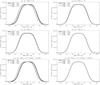Fig. 3 Time variation in the Hα spectral line profile for consecutive phases (labelled in the top left corner of each plot) and different modes. The two bottom plots correspond to modes with vx variations only, where we assumed T = const. and p = const. Specific line intensities are in cgs units erg s-1 cm-2 sr-1 Hz-1.

Fig. 4 Same as Fig. 3, but for Hβ.

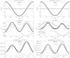Fig. 5 Time variation as a function of phase of the spectral line parameters for all modes. Different lines labelled in the plots correspond to different modes.

Fig. 6 Same as Fig. 5, but for T = const. and p = const.

Using the prescribed time-dependent MHD model, we performed this NLTE transfer modeling for a hydrogen model atom having five bound levels and continuum. For a static case, this type of modeling is described in Heinzel (1995) and summarized in Labrosse et al. (2010). Present computations have been performed assuming the complete redistribution in Lyman lines. We took the height of the line of sight above the limb to be 10 000 km, which determines the dilution of the incident radiation. For the sake of simplicity, we set the microturbulent velocity to zero; for more realistic values, the line-center optical thickness (τ) will decrease.

4. Results

We have obtained time-dependent series of generally asymmetrical line profiles of the hydrogen Hα (Fig. 3) and Hβ lines (Fig. 4). Hα is saturated (flat line core) because the line-center optical thickness is around 4, while Hβ has an almost Gaussian shape and is about an order of magnitude thinner, i.e. τ₀ < 1 (the line-center optical thickness). For some other models with different temperatures and gas pressures, a central reversal may be present in Hα as in the set of static models of Gouttebroze et al. (1993). From the set of profiles, we clearly see periodic oscillations in both the line intensity (due to temperature and pressure variations) and in the wavelength position or asymmetry. These variations have to be compared with spectral observations of oscillating prominences (see Zapiór & Kotrč 2012).

We have to distinguish between two notions: the optical thickness and the optical depth. The optical depth is defined as: $\mathrm{d}\mathit{\tau }\mathrm{\left(}\mathit{\lambda }\mathrm{\right)}\mathrm{=}\mathit{\kappa }\mathrm{\left(}\mathit{\lambda }\mathrm{\right)}\mathrm{d}\mathit{x,}$(11)where κ(λ) is the wavelength-dependent absorption coefficient. In the case of quiescent prominences, its profile is practically Gaussian but Doppler-shifted due to local oscillatory motions. For the radiative-transfer modeling we transform the x-scale from (− x₀,x₀) (shown in Fig. 1) to (0,2x₀). The optical depth is then 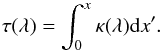$\mathit{\tau }\mathrm{\left(}\mathit{\lambda }\mathrm{\right)}\mathrm{=}{\mathrm{\int }}_{\mathrm{0}}^{\mathit{x}}\mathit{\kappa }\mathrm{\left(}\mathit{\lambda }\mathrm{\right)}\mathrm{d}{\mathit{x}}^{\mathrm{\prime }}\mathit{.}$(12)The optical thickness is simply the optical depth at x = 2x₀, which corresponds to thickness of the whole prominence slab. Both quantities vary from the line center towards the line wings. In the line center, the slab is most opaque, while it becomes gradually more and more transparent by going to the wings. This has principal consequences on the analysis of the synthetic (and also observed) profiles because in the optically-thick regime (i.e. for τ(λ) > 1) we can “see” the moving plasma only down to optical depths around unity. In cases when the slab is optically thin (τ(λ) < 1), we detect the motions from all depths, and the resulting line profile is a superposition of all depth-dependent contributions. In the model studied here, the Hα line-center optical thickness of the whole slab is around 4 in the approximation of the complete frequency redistribution used here for simplicity and neglecting the microturbulent velocity, see discussion in Sect. 5.

The only evident asymmetry is detectable in Hα for the fundamental slow mode (fS), and namely for phases 0. and 0.5 (see top left panel in Fig. 3). We clearly see the line asymmetry and a well resolved Doppler shift. For the first slow overtone (1S), these velocity-induced changes are much less evident and the line profiles are dominated by thermodynamic perturbations. To understand this behavior better, we have made the following numerical experiment: we set all depth-dependent variations in temperature and gas pressure to zero and considered a simple isothermal-isobaric slab characterised by the unperturbed thermodynamic quantities. Then by using the same velocity fields as in the exact case, we calculated spectral profiles in the same way. The obtained profile variations with time for fS and 1S are plotted at the bottom of Fig. 3. While the fS shows similar Doppler effects as before (only the line center intensity is not varying), the 1S case exhibits no variations. This clearly shows that the profile variations are significantly affected by oscillations (always having the same sign at a given time) in the case of fS. For 1S model the dominant role is played by temperature/pressure changes and the effect of oscillatory motions is damped because of the antisymmetric variations along x (Fig. 2). The same behavior is seen for Hβ in Fig. 4. For fundamental fast mode (fF) and first fast overtone (1F), the situation is even less favorable – we see only small profile variations due to temperature-pressure changes.

From the computed line profiles of Hα and Hβ, we derived three line parameters: Doppler shift, maximum intensity, and full width at half maximum (FWHM). At the beginning, we approximate discrete points of the line profiles with the function $\mathit{I}\mathrm{\left(}\mathit{\lambda ,t}\mathrm{\right)}\mathrm{=}\mathit{S}\left[\mathrm{1}\mathrm{-}{\mathrm{e}}^{\mathrm{-}{\mathit{\tau }}_{\mathrm{0}}{\mathrm{e}}^{\mathrm{-}{\left(\frac{\mathit{\lambda }\mathrm{-}{\mathit{\lambda }}_{\mathrm{0}}\mathrm{+}\mathrm{\Delta }{\mathit{\lambda }}_{\mathit{V}}}{\mathrm{\Delta }{\mathit{\lambda }}_{\mathrm{D}}}\right)}^{\mathrm{2}}}}\right]\mathit{,}$(13)where I(λ) is the line profile, S the source function, τ₀ line-center optical thickness, λ₀ is the wavelength of the line center, Δλ_V Doppler shift of the line profile, and Δλ_D is the Doppler width. This expression represents the formal solution of the transfer equation with a constant line source function. We treated S, τ₀ , Δλ_V, and Δλ_D as free parameters. The maximum intensity of the spectral line was set to a peak value of the line profile. Since the spectral profiles were calculated with certain accuracy, the corresponding plots exhibit some noise. We also determined FWHM, where the noise is also caused by the numerical accuracy. Since the Doppler shift was calculated as a free parameter of the approximated curve, it is not so affected by such noise. All parameter variations are shown in Fig. 5 and summarized in Tables 1 and 2. We detected substantial Doppler shifts for fS only with a peak-to-peak value of about 2 km s^-1, which is about a half the amplitude of plasma motions in the central part of the slab. The line FWHM shows slightly asymmetrical behavior in both lines and its amplitude is small. Finally, the maximum line intensity is better detectable (variations about 10% and more) in the Hβ line simply because Hα is saturated. We have done numerical test for fS and 1S modes with T(t) = T₀ = const. and p(t) = p₀ = const. Results are plotted in Fig. 6. Doppler shifts are almost the same which means that they are not affected by variations in the thermodynamic parameters. However, FWHM and the maximum intensity look quite differently. This suggests that Hβ maximum intensity can be a good indicator of T and p variations.

Fast modes (fF and 1F) have a negligible Doppler shift, as expected from a very low amplitude of v_x, and because the prominence axis is perpendicular to the line-of-sight. Fast modes cause plasma motions that are mainly in vertical direction parallel to the axis of the slab. As mentioned before, the model 1S has also a negligible Doppler shift, which could be explained in the following way. The Hα line center is optically thick, but a certain fraction of radiation comes from central parts of the slab in line wings. Since both the surface and the slab center have zero velocities for 1S models, the contributions to the Doppler signal from those regions are negligible. The models fS, f,F and 1S give rise of Hα peak-to-peak FWHM variations in about 4–5% and 1–2% for the Hβ. The peak-to-peak maximum intensity changes are about 3–4% for Hα and 10–18% for Hβ also for modes fS, fF, and 1S. Especially for Hβ, these changes are detectable. Other cases are negligible.

5. Summary and future prospects

In this study we have performed, for the first time, numerical simulations of the NLTE radiative transfer in oscillating prominence slabs to investigate changes of the spectral profiles. As the input, we used the MHD models that describe various modes of global oscillations within simple 1D slabs. These slabs, which represent prominences as seen on the solar limb, are strongly illuminated by the radiation from the solar disk and this radiation is scattered by the prominence plasma. We have considered the hydrogen plasma and computed the synthetic spectral line profiles of two Balmer lines, Hα and Hβ, which are the most frequently observed optical lines in prominences. The model considered here has typical temperatures and gas pressures, and we have obtained a reasonable Doppler signal for the fundamental slow mode. Detected peak-to-peak amplitudes of velocities are of the order of 2 km s^-1, while the real one of the MHD model is 4 km s^-1. The difference results from a response of the slab atmosphere to specific oscillations. Note that such velocities have been recently detected by Zapiór & Kotrč (2012). We detected variations in the maximum intensity and FWHM for the fundamental slow mode and its first overtone and the fundamental fast mode, which are caused by temporal changes of the thermodynamic quantities, namely the temperature and gas pressure. Only the first fast overtone is practically non-detectable for all observables.

In this exploratory study, we did not consider the height variations (along the z-coordinate). To obtain a realistic distribution of the radiation field, atomic-level populations and electron densities, one should solve the 2D transfer problem, as described for prominences by Paletou (1995) and Heinzel & Anzer (2001).

The next step of the investigations may deal with the sensitivity of the line profile to a particular velocity perturbation at a certain depth, which is usually described by the so-called velocity response function (e.g. Mein 2000). In the future, a more rigorous treatment with the partial frequency redistribution (PRD) in hydrogen Lyman lines will be used. This leads to an increase in τ roughly by factor of two in the Hα line center, as our test on current oscillatory models have indicated. However, non-zero microturbulent velocities (not considered here) act in the opposite direction, lowering the optical thickness. Therefore, complete redistribution together with zero microturbulence mimics more realistic situations somehow. The presence of velocity fields also makes the radiative transfer problem with the PRD more complex, and we thus postpone this issue to further studies. The MHD model will be more realistic by considering immersion of the slab in a coronal environment with partially ionized plasma inside the slab. Partial ionization will also make it more consistent with the radiation transfer model we used in this study.

The prominence magnetic field is consistently incorporated into the MHD model but has no explicit effect on the synthetic line profiles. However, an exploration of wider range of models and comparison to relevant observations could lead to a realistic diagnostics of the magnetic field structure. Simultaneous polarimetric observations would then be extremely important to compare the results, since the prominence seismology might serve as an independent diagnostics of the magnetic fields. We have used only one specific initial temperature and gas pressure; other thermodynamic models would lead to different results. For example, we could better disentangle between the surface and internal dynamics of the slab by increasing the optical thickness in Hα. On the other hand, our model example is already opaque with p = 0.02 Pa and the total geometrical thickness D = 12   000 km (which is large compared to typical values for quiescent filaments). Therefore, it is evident that some other spectral lines of other species, which are even optically thicker than Hα might be quite useful to diagnose the oscillations. Namely, we have in mind the Ca ii H and K lines, which are optically thick and are easily detectable from the ground. New perspectives also appear in connection with the IRIS space mission, where the UV spectrometer covers strong and optically thick Mg ii h and k lines (Heinzel et al. 2014). Since IRIS provides a high temporal resolution, the prominence oscillations should be well detectable.

Acknowledgments

P.H. and M.Z. acknowledge support from the Grant Agency of the Czech Republic through grant 209/12/0906. This work was also supported by the institute project RVO 67985815. M.Z. thanks the Astronomical Institute at Ondřejov for their hospitality and support. J.L.B., R.O., and M.Z. acknowledge financial support provided by MICINN and FEDER funds under grant AYA2011-22846. J.L.B. and R.O. acknowledge financial support from CAIB and Feder Funds under the “Grups Competitius scheme”. The authors thank the referee for valuable comments.

References

All Tables

All Figures

Fig. 1 Sketch of the geometry of the considered problem common for the MHD simulation and for the radiative transfer. The prominence slab with infinite height and length and width 2x0 is penetrated by a constant magnetic field. For a radiative transfer, we should take into account incident radiation from the surface (dashed arrows), according to the position above the solar limb (h). The line-of-sight is perpendicular to the slab.

In the text

Fig. 2 Velocity perturbations along the x-axis of the slab for the fundamental slow mode (fS, top left), the first slow overtone (1S, top right), the fundamental fast mode (fF, bottom left) and the first fast overtone (1F, bottom right). The x-axes of plots are scaled in meters. Note the different velocity scale. Different lines represent different phases (i.e. time divided by period), as labelled at the top left corner of each plot. For phase =0.25 and phase =0.75, the lines are merged. Oscillatory periods are shown at the top right corner of each plot.

In the text

	Fig. 3 Time variation in the Hα spectral line profile for consecutive phases (labelled in the top left corner of each plot) and different modes. The two bottom plots correspond to modes with vx variations only, where we assumed T = const. and p = const. Specific line intensities are in cgs units erg s-1 cm-2 sr-1 Hz-1.
In the text

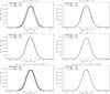	Fig. 4 Same as Fig. 3, but for Hβ.
In the text

	Fig. 5 Time variation as a function of phase of the spectral line parameters for all modes. Different lines labelled in the plots correspond to different modes.
In the text

	Fig. 6 Same as Fig. 5, but for T = const. and p = const.
In the text

References

- Arregui, I., & Ballester, J. L. 2011, Space Sci. Rev., 158, 169 [NASA ADS] [CrossRef] [Google Scholar]
- Arregui, I., Oliver, R., & Ballester, J. L. 2012, Liv. Rev. Sol. Phys., 9, 2 [Google Scholar]
- Balthasar, H., & Wiehr, E. 1994, A&A, 286, 639 [Google Scholar]
- Balthasar, H., Knoelker, M., Wiehr, E., & Stellmacher, G. 1986, A&A, 163, 343 [NASA ADS] [Google Scholar]
- Banerjee, D., Erdélyi, R., Oliver, R., & O’Shea, E. 2007, Sol. Phys., 246, 3 [NASA ADS] [CrossRef] [Google Scholar]
- Berlicki, A., Heinzel, P., Schmieder, B., Mein, P., & Mein, N. 2005, A&A, 430, 679 [NASA ADS] [CrossRef] [EDP Sciences] [Google Scholar]
- Gouttebroze, P., Heinzel, P., & Vial, J. C. 1993, A&AS, 99, 513 [NASA ADS] [Google Scholar]
- Heinzel, P. 1995, A&A, 299, 563 [NASA ADS] [Google Scholar]
- Heinzel, P., & Anzer, U. 2001, A&A, 375, 1082 [NASA ADS] [CrossRef] [EDP Sciences] [Google Scholar]
- Heinzel, P., Vial, J.-C., & Anzer, U. 2014, A&A, in press [Google Scholar]
- Labrosse, N., Heinzel, P., Vial, J.-C., et al. 2010, Space Sci. Rev., 151, 243 [Google Scholar]
- Landman, D. A., Edberg, S. J., & Laney, C. D. 1977, ApJ, 218, 888 [NASA ADS] [CrossRef] [Google Scholar]
- Mackay, D. H., Karpen, J. T., Ballester, J. L., Schmieder, B., & Aulanier, G. 2010, Space Sci. Rev., 151, 333 [NASA ADS] [CrossRef] [Google Scholar]
- Mein, P. 2000, in Proc. NATO ASI Adv. Sol. Res. Eclipses from Ground and from Space, eds. J.-P. Zahn, & M. Stavinschi (Dordrecht: Kluwer), NATO Science Ser. C, 558, 221 [Google Scholar]
- Nejezchleba, T. 1998, A&AS, 127, 607 [NASA ADS] [CrossRef] [EDP Sciences] [Google Scholar]
- Oliver, R. 1999, in Magnetic Fields and Solar Processes, eds. A. Wilson et al., ESA SP, 448, 425 [Google Scholar]
- Oliver, R. 2009, Space Sci. Rev., 149, 175 [NASA ADS] [CrossRef] [Google Scholar]
- Oliver, R., & Ballester, J. L. 2002, Sol. Phys., 206, 45 [NASA ADS] [CrossRef] [Google Scholar]
- Oliver, R., Ballester, J. L., Hood, A. W., & Priest, E. R. 1992, ApJ, 400, 369 [NASA ADS] [CrossRef] [Google Scholar]
- Paletou, F. 1995, A&A, 302, 587 [NASA ADS] [Google Scholar]
- Suematsu, Y., Yoshinaga, R., Terao, N., & Tsubaki, T. 1990, PASJ, 42, 187 [NASA ADS] [Google Scholar]
- Suetterlin, P., Wiehr, E., Bianda, M., & Kueveler, G. 1997, A&A, 321, 921 [NASA ADS] [Google Scholar]
- Tsubaki, T. 1988, in Proc. Solar and Stellar Coronal Structure and Dynamics, ed. R. C. Altrock, Sol. Phys., 140 [Google Scholar]
- Tsubaki, T., & Takeuchi, A. 1986, Sol. Phys., 104, 313 [NASA ADS] [CrossRef] [Google Scholar]
- Tsubaki, T., Ohnishi, Y., & Suematsu, Y. 1987, PASJ, 39, 179 [NASA ADS] [Google Scholar]
- Tsubaki, T., Toyoda, M., Suematsu, Y., & Gamboa, G. A. R. 1988, PASJ, 40, 121 [NASA ADS] [Google Scholar]
- Wiehr, E., Balthasar, H., & Stellmacher, G. 1984, Sol. Phys., 94, 285 [NASA ADS] [CrossRef] [Google Scholar]
- Yi, Z., Engvold, O., & Keil, S. L. 1991, Sol. Phys., 132, 63 [NASA ADS] [CrossRef] [Google Scholar]
- Zapiór, M., & Kotrč, P. 2012, Central European Astrophysical Bulletin, 36, 89 [NASA ADS] [Google Scholar]