| Issue |
A&A
Volume 562, February 2014
|
|
|---|---|---|
| Article Number | A41 | |
| Number of page(s) | 13 | |
| Section | Galactic structure, stellar clusters and populations | |
| DOI | https://doi.org/10.1051/0004-6361/201117339 | |
| Published online | 04 February 2014 | |
Proper motions for HST observations in three off-axis bulge fields⋆
1 Space Telescope Science Institute, 3700 San Martin Drive, Baltimore, MD 21218, USA
e-mail: This email address is being protected from spambots. You need JavaScript enabled to view it.
2 Leiden Observatory, Leiden University PO Box 9513, 2300 RA Leiden, The Netherlands
e-mail: This email address is being protected from spambots. You need JavaScript enabled to view it.
3 Departamento de Física, Universidad de La Serena, 980 Benavente, La Serena, Chile
4 Departamento de Astronomía, Universidad de Chile, 36-D Casilla, Santiago, Chile
e-mail: This email address is being protected from spambots. You need JavaScript enabled to view it.
5 Leibniz-Institut für Astrophysik Potsdam (AIP), an der Sternwarte 16, 14482 Potsdam, Germany
e-mail: This email address is being protected from spambots. You need JavaScript enabled to view it.
6 Max Planck Institute for Astronomy, Königstuhl 17, 69117 Heidelberg, Germany
e-mail: This email address is being protected from spambots. You need JavaScript enabled to view it.
Received: 25 May 2011
Accepted: 27 August 2013
Abstract
Aims. This is the second in a series of papers that attempt to unveil the kinematic structure of the Galactic bulge through studying radial velocities and proper motions. We report here ~15 000 new proper motions for three low foreground-extinction off-axis fields of the Galactic bulge.
Methods. Proper motions were derived from a combination of Hubble Space Telescope Wide Field Planetary Camera 2 (WFPC2) and Advanced Camera for Surveys (ACS) images taken 8 and 9 years apart, and they reach accuracies better than 0.9 mas yr-1 for more than ~10 000 objects with magnitudes F814W ≤ 24.
Results. The proper motion distributions in these fields are similar to those of Galactic minor axis bulge fields. We observe the rotation of main sequence stars below the turn-off within the Galactic bulge, as in the minor axis fields.
Conclusions. Our stellar proper motions measurements show a significant bulge rotation for fields as far from the Galactic plane as b ≃ −8°.
Key words: Galaxy: bulge / Galaxy: kinematics and dynamics / Galaxy: stellar content / methods: data analysis
Based on observations made with the NASA/ESA Hubble Space Telescope, obtained from the data archive at the Space Telescope Institute. STScI is operated by the association of Universities for Research in Astronomy, Inc. under the NASA contract NAS 5-26555.
© ESO, 2014
1. Introduction
It is still uncertain exactly what mechanisms led to the formation of the present-day Galactic bulge. It is not clear whether the evolution of the bulge was driven by mergers, as the hierarchical galaxy formation scenarios suggest, or secularly by disk instabilities. A clear observational picture of the bulge’s current structure is needed to begin to understand its formation and evolution. Because of the high and variable extinction towards the Galactic center, this has been a difficult task and is perhaps the main obstacle to formulating a unified picture. In addition to the high foreground extinction by dust towards the Galactic bulge (which is not constant even on small scales), the bulge and the disk are projected on top of each other on the sky. Disentangling them is not straightforward: even in the color-magnitude diagram (CMD), the populations overlap (Holtzman et al. 1998). Moreover, blue stragglers extend brighter than the turn-off and overlap with the main sequence region hosting the young population. This complicates the separation of populations based on photometry alone, and additional measurements are required to accurately study the different components of the bulge.
Despite these difficulties, progress has been made in understanding the Galactic bulge, especially over the past years. Abundance studies, such as those by Rich (1988), McWilliam & Rich (1994), Zoccali et al. (2008), and Bensby et al. (2011), have shown that the Galactic bulge has a wide range of metallicities. However, bulge metallicities do typically differ from disk and halo populations, showing a comparatively metal-rich population. The α-elements in the bulge have also been consistently found to be overabundant with respect to halo and disk (Zoccali et al. 2006; Fulbright 2007; Hill et al. 2011). In particular, α-elements are related to the formation timescale of the Galactic bulge since they are primarily produced during the explosion of SN Type II (due to short-lived massive stars). Iron production, on the other hand, is favored by SNe Type Ia explosion, where SN Type Ia typically have a timescale of an order of magnitude longer than SN Type II. Therefore, the overabundance of α-elements in the bulge suggests a rapid formation scenario. Evidently, most bulge stars were formed before the interstellar medium (ISM) could be enriched by SN Type Ia explosions, hence the short inferred formation timescale for the bulge (<1 Gyr) (e.g. Ballero et al. 2007, and references therein).
Simulations in the last few years have also complicated our view of the formation scenarios of the Galactic bulge. Shen et al. (2010) reproduced the stellar kinematics of the Bulge Radial Velocity Assay (BRAVA; Rich et al. 2007) without a classical bulge, where the boxy bulge previously reported in the literature is the end-on projection of the bar structure. Conversely, Saha et al. (2012) finds that a non-rotating small classical bulge can evolve secularly through angular-momentum exchange with the Galactic bar.
At the same time, number counts along the CMD between populous clusters at several latitudes have been used to estimate the foreground disk contamination (Feltzing & Gilmore 2000) and the age of the bulge. The foreground disk population mimics the young bulge population, especially near the turn-off, affecting the age determinations in the bulge. The results for two bulge fields that effectively identified the contamination by foreground populations have placed the age of the bulge population as old as ~10 Gyr.
Summary of observations.
Despite its proximity, the Galactic bulge has classically suffered from a lack of proper-motion studies. Spaenhauer et al. (1992) were the first to obtain reliable proper motions from a Galactic bulge sample using photometric plates taken more than three decades apart. This study was the subject of a subsequent analysis by Zhao et al. (1994), who included radial velocities for a small subsample (64 stars). They found a significant vertex deviation (i.e., a triaxility signature) for the metal-rich population in their small proper motion-radial velocity combined sample. The same signature of triaxility was observed by Soto et al. (2007), who combined Spaenhauer et al. (1992) proper motions with Sadler et al. (1996) and Terndrup et al. (1995) radial velocities and metallicities to obtain a sample of ~300 K giants with 3D kinematics and metallicities. More recently, the same triaxility signature related to two distinct populations, metal-rich and metal-poor, has been confirmed using high-resolution spectra by Babusiaux et al. (2010) and Hill et al. (2011).
Microlensing surveys of the Milky Way bulge have also contributed to improving our knowledge of the kinematics of the Galactic bulge. The OGLE-II experiment has produced ~5 × 10⁶ proper motions (Sumi et al. 2004) for 49 bulge fields, covering a range of − 11° < l < 11° and − 6° < l < 3°, and reaching accuracies of 0.8 − 3.5 mas yr-1. Using this survey as a basis, Rattenbury et al. (2007a,b) studied the proper motions for a subsample of bulge red clump giant stars in 44 fields. Red clump stars were used as tracers of bulge density in order to fit a mass density distribution for the bulge. Along the same lines, Vieira et al. (2007) delivered proper motions for 21 000 stars in Plaut’s window (l,b = 0°, − 8°) from plates spanning 21 years.
Space-based observations have also played a role in bulge proper-motion observations, boasting the combination of sharper images and reduced blending. Anderson & King (2000, 2003) developed a technique of deriving precision astrometry. Their innovations included an effective point spread function (PSF) approach that obviates the need to integrate the PSF over pixels when evaluating it for a given image, and an empirical distortion correction for WFPC2, later on extended to the ACS Wide-Field Channel (WFC) and ACS High-Resolution Channel (HRC). These procedures were subsequently applied to measuring the component of rotation of 47 Tucanae globular cluster (Anderson & King 2003). Similarly, Kuijken & Rich (2002; henceforth KR02) used a modification of Anderson & King (2000) approach to be the first to use Hubble Space Telescope (HST) observations to obtain reliable bulge proper motions. KR02’s sample targeted two low foreground-extinction fields, Baade’s window (l,b = 1.1°, − 3.8°) and Sagittarius I (l,b = 1.3°, − 2.7°).
Both fields were used to successfully obtain 15 862 and 20 234 proper motions, respectively, proving the feasibility of space-based proper motions with considerably shorter time baselines than those previously employed on ground-based bulge proper motions (e.g., Spaenhauer et al. 1992; ~30 yr). The samples in both fields were separated into bulge and disk components based on the mean proper motions. From this it was found that the bulge component clearly resembles an old population, such as those observed in globular clusters, and shows a significant rotation with no covariance in l,b. More recently, both fields in KR02 have been the subject of new proper motion studies. Kozłowski et al. (2006) obtained proper motions for 35 small fields in the vicinity of Baade’s window. Their calculations, involving the combination of ACS/HRC images and archival observations with WFPC2, yielded 15 863 stellar proper motions. The proper motions calculated by Kozłowski et al. (2006) show consistency with the velocity dispersions found by KR02, and in addition show a significant negative covariance term in the transverse velocity Clb = σlb/(σlσb) ≃ − 0.10. A negative covariance such as this may imply a tilt in the velocity ellipsoid with respect to the Galactic plane.
Similarly, new results for the Sagittarius I field (Clarkson et al. 2008) yielded more than 180 000 proper motions with ACS epochs separated by just 2 years. From their initial numbers they finally selected 15 323 bulge stars using a similar procedure to the one applied by KR02. The covariance they report was very similar to the one found by Kozłowski et al. (2006). In addition, Clarkson et al. (2008) produced velocity ellipsoids in (l,b) as a function of distance bins. These velocity ellipsoids demonstrate a slight dependence on the distance of the objects analyzed. Similar to the finding in KR02, the median stellar sequence in Clarkson et al. (2008) for this bulge sample was best represented by an 11 Gyr old isochrone.
We report here new proper motions results for stars in three low foreground-extinction windows of the Galactic bulge located in the first Galactic quadrant. These new fields differ from other HST bulge proper motion observations, such as the minor-axis fields presented in Clarkson et al. (2008) and KR02, since they sample the near end of the bar in the Galactic bulge. In addition, the derived proper motions have been obtained from cross-detector observations; suitable first-epoch WFPC2 exposures were obtained from the HST archive, and complemented with more recent ACS WFC exposures. These second-epoch observations are part of a larger program (GO-9816) that includes observations in both ends of the Galactic bar, as well as minor axis fields (see Soto et al. 2012, for more details). The resulting time baselines for the proper motions in this work are eight to nine years.
This paper is organized as follows. In Sect. 2 we describe our observations. A detailed account of the procedures involved in the measurements of the proper motion can be found in Sect. 3. Section 4 presents the analysis performed on our sample of proper motions and the implications of the results. In addition, we compare our results with those of similar surveys in the Galactic bulge. Finally, our conclusions are summarized in Sect. 5.
2. Observations
Our observations target three fields at positive Galactic longitudes; Field 4-7 [(l,b) = (3.58°, −7.17°)], Field 3-8 [(l,b) = (2.91°, −7.96°)], and Field 10-8 [(l,b) = (9.86°, −7.61°)]. First-epoch observations were obtained from the HST data archive, which is now over a decade and a half old. In addition to the three fields analyzed here, this wealth of images also provided the basis for the three low foreground-extinction fields close to the Galactic minor axis; these results are reported in KR02 and Kuijken (2004; henceforth K04). Two aspects of the first-epoch data are not ideal: (i) the exposures are all long (>1200 s), so the positions of the bright stars are not measurable; (ii) the exposures are not dithered, which limits our ability to build a PSF model. To mitigate the effect of the undersampling of the PSF, we chose the F814W filter that has the widest, hence the least, undersampled PSF.
The observations for our three fields have combined WFPC2 and ACS WFC for the first and second epochs, respectively. ACS WFC observations were preferred for the second-epoch, in spite of the cross-instrument systematics, owing to their extended field and the resolution which an eventual third ACS epoch could take advantage of. The ACS WFC second-epoch observations were acquired during 2004 July 12 and 14. Two short exposures with 50 s of integration time and four longer exposures of ~350 s were taken for each field. These observations were dithered using a line pattern for the 50 s exposures, while a box pattern was chosen for the longer 347 s exposures, and spacings in each case were set to (0.1825) arcsec and (0.265,0.187) arcsec, respectively. These ACS second-epoch observations are not completely aligned with the WFPC2 first-epoch. Inclination angles of ~14° for fields Field 4-7 and Field 3-8, and ~17° for Field 10-8 were measured. Table 1 summarizes our observation in both epochs for our three fields.
It has been demonstrated that for a wide range of realistic PSF profiles, the 1σ uncertainty in the centroid of a stellar images of full width at half maximum (FWHM), and signal-to-noise ratio (S/N) is given by ≃ 0.7 × FWHM/(S/N) (KR02). This theoretical limit gives us a reference for what can be expected in our proper motions, for first-epoch observations were performed in WFPC2 (FWHM ≃ 0.12′′ in F814W) a star detected at 15σ can be centered with a precision of 5.6 mas. Therefore, a time baseline of 8 yr (in our fields we have 8−9 yr of baseline) yields an accuracy of 0.53 mas yr-1, which corresponds to ~20 km s-1 at the distance of the bulge (~8 kpc). Since our second-epoch observations are dithered and are of a higher resolution, they reach higher accuracies than those of the first epoch. However, the latter cannot improve our proper motion accuracy beyond the limits of the first epoch, and the spatial variations in the PSF within the ACS WFC image (Anderson & King 2006) have not been considered in our analysis. These PSF spatial variations in ACS, if ignored, can produce 10% of error in core photometry, which is reduced when a larger aperture is taken. In the case of astrometric measurements, the effects are at the 0.01 pixel level (≃ 0.001′′ for ACS), which is negligible considering the error introduced by the first epoch. New measurements including only ACS measurements will include this effect in our astrometric measurements in the future. Similarly, another possible source of uncertainty in our proper motion solution can be the charge transfer efficiency (CTE) problem in WFPC2 (Dolphin 2000) and ACS (Kozhurina-Platais et al. 2007). The CTE effect has been carefully characterized for both cameras, and it is known to affect the astrometric precision, as well as the photometric accuracy. However, this effect should not be significant for images taken during 1994−1995 (WFPC2) and 2004 (ACS), where the instruments had less than ~1 and ~2 yr in orbit, respectively. This has also been demonstrated for the proper motions of KR02 and Clarkson et al. (2008) for other bulge fields.
3. Proper motion measurements
Anderson & King (2000) describe a procedure for accurate astrometric measurements using HST WFPC2, and they subsequently updated this technique for ACS WFC (Anderson & King 2006). Originally these techniques were designed to work with both epochs dithered, where a common PSF model is used for all the dithered exposures. This PSF must be consistent with all the exposures and is used to obtain the centroids of each star. Our data, on the other hand, with its undithered first-epoch observations, have required some modifications to the original Anderson & King (2000) recipe. To improve the centroid determination, we determine a PSF for each exposure starting from an analytical model. This model consists of a Gaussian PSF multiplied by a polynomial, where the number of the components for the polynomial accounts for the wings of the PSF and other secondary features: three polynomial components in a three-pixel fitting radius for WFPC2/WF exposures, and 12 polynomial components in a five-pixel fitting radius for WFPC2/PC or ACS/WF exposures. For each exposure, therefore, the PSF starts from this analytical model and is fitted to the 100 brightest, unsaturated stars in the image. Our process then iterates using a higher order polynomial, with an robust outlier rejection, which refines the selection until it converges. Typically, a minimum of ten iterations have been run to fit the PSF model.
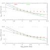 |
Fig. 1 The rms residuals of the pixels positions in x (bottom) and y (top) from the proper motion fits in one of our fields, Field 4-7 WF2. The solid lines are the best theoretical fit for an error estimation based on photon noise alone (bottom line) and for photon noise including additional systematic source of errors for each epoch (top two lines). This plot shows that the dominant source of error for the fainter undithered first epoch (red) is photon noise, while for brighter sources a residual systematic error appears that we relate to saturation due to the long exposures. Second-epoch dithered exposures (green) are best represented by a systematic error that has been included in the estimation of the proper motion error. |
Once the PSF has been calculated for each exposure, the proper motions can be determined. These are obtained starting from a master image that has been generated by combining all the flat-fielded *_flt WFPC2, first-epoch (undithered) exposures in the F814W filter. The combined master image is then run through DAOFIND to detect stars with fluxes over 15σ, which produces a master list of stars. This master list is used to detect the same stars in all the exposures in both epochs; for each exposure, the master list coordinates are used as an initial guess to determine the star position. In the case of WFPC2 first-epoch exposures, a simple linear transformation is sufficient to transform the master-list coordinates to each exposure (e.g., KR02). On the other hand, for our second-epoch ACS WFC images, we have used a third-order polynomial transformation, constructed with the IRAF task GEOMAP, to convert the master-list WFPC2 positions to the ACS/WFC second-epoch exposures. This procedure does not affect the final proper motion result as long as the transformed master-list coordinates for the second-epoch allow a unique identification of the same star in all the second-epoch exposures. For each star, a PSF fit is then computed for the initial positions derived from the converted master list coordinates, to give a best fitting position in each exposure of both epochs.
These positions on each exposure are then aligned to a common reference frame by fitting a polynomial to each of the sets of coordinates of bright unsaturated stars. With the positions calculated for each exposure in the reference frame, it is straightforward to then extract the proper motions. First the proper motions must be separated from the rest of the effects included within these positions. These include a general transformation that maps the positions of each exposure to those of the reference frame, which also includes the residuals of the geometric distortion of the individual frames, the proper motions, the average position residual as a function of pixel phase for each image that is subtracted from each measurement, and the average residual position as a function of the “34th row” effect (Anderson & King 1999). This process is iterative, and produces a proper motion solution in each loop for each star. This solution is obtained from a weighted linear least-square fit with rejection of outliers, where the weights are estimated from the centroid errors, which are in turn estimated based on photon noise and systematic residual errors. Figure 1 shows an example of the the rms residuals of the positions in one of our fields (Field 4-7), in the chip WF4. While the dominant source of error for the faint stars in the first undithered epoch seems consistent with photon noise, the brighter stars include a systematic residual. On the other hand, the second epoch (properly dithered) exposures show residuals consistent with a systematic error, which have been correctly considered in our proper motion solution. In both cases we have found that for the fainter end, the systematic errors are below ~0.8 mas yr-1 for a baseline of 9 yr, which at a distance of 8 kpc corresponds to ~30 km s-1. A more detailed account of the technique can be found in KR02, so will not be repeated here.
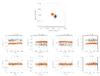 |
Fig. 2 Kinematic selection of cluster stars in Field 10-8 in one of the cameras of WFPC2, Wide Field 4 (WF4). The selection was performed for each chip separately using a hard cut-off; cluster stars have a small velocity dispersion, which therefore biases the relative zeropoint of the proper motions of bulge stars. Thus, the cluster stars must be excluded from the reference frame used to calculate bulge proper motions. Top panel: proper motions in pixel yr-1 before the refinement of the stars used as the basis for the inter-epoch transformations for WF4 chip in Field 10-8; where black dots are bulge stars, and orange dots are those kinematically classified as cluster stars. Second row: proper motions in pixels μx and μy as a function of the x − y coordinates before the correction. Bottom row: same as the second row, but after applying the correction. |
We must stress that these are relative proper motions, because they assume that the average movement of all the stars in the field is zero. Absolute proper motions would require identifying of extragalactic sources to use as references in the same field. The zero-mean assumption works well for bulge fields, but breaks down when many stars have the same peculiar velocity. Such is the case of the Field 10-8, where many of the bright stars in the master list correspond to the globular cluster NGC 6656 (M22). To make matters worse, the mean proper motion is different for the four chips of WFPC2 since the cluster star fraction depends on position. To remove this effect, the cluster stars in each image are removed from the master list by identifying the cluster stars from the proper motions calculated from all the stars in the field. Taking advantage of the small proper motion dispersion of the cluster, the NGC 6656 stars can be easily identified (and removed). The proper motions are then calculated again using only non-cluster stars, in which it is reasonable to use the assumption of average movement zero. This procedure is illustrated in Fig. 2 for one of the chips, WF4. In a similar way, we repeated the latter procedure for cluster stars in order to exclude bulge contamination.
3.1. NGC 6656 proper motions
In a globular cluster, the velocity dispersion observed must be small to maintain a dynamically stable structure. This is consistent with the previously reported kinematics in NGC 6656; the Catalog of Parameters for Milky Way Globular Clusters (Harris 1996) lists a velocity dispersion of ~7.8 km s-1 for NGC 6656, based on radial velocities. Similarly, Peterson & Cudworth (1994) reported a velocity dispersion of 6.6 ± 0.8 km s-1 for stars within a 1′ − 7′ annular field, and a proper motion dispersion of 0.56 ± 0.03 mas yr-1, the latter corresponding to ~8.5 ± 0.5 km s-1 using a distance of 3.2 kpc (Samus et al. 1995). More recently, Chen Ding et al. (2004) have used HST WFPC2 observations to obtain a proper motion dispersion  mas yr-1, or 17 km s-1.
As mentioned before, Field 10-8 was separated into a cluster and a bulge component during the proper motion procedure by means of a pure kinematic selection. This kinematic selection was performed for each chip by selecting a small radius around the cluster proper motions (see Fig. 2), where our WFPC2 fields sample cluster stars in a radius between ~2′ and ~5′ from the center of NGC 6656. Table 2 and Fig. 3 show the number of cluster stars selected per field and proper motion dispersions, while Fig. 4 shows the respective binned CMD. Our first impression is that these plots do not indicate significant gradients or variations, as expected of a globular cluster, and seem consistent with the previously listed literature. Furthermore, the small dispersion observed in our cluster proper motions results, combined with the reported kinematics, can be used as an external assessment of the accuracy of our procedures.
Table 2 indicates a dispersion in l and b of ~1.04 mas yr-1 for cluster stars at the WF chips, which corresponds to ~17 km s-1. The PC dispersions are about twice as small, a fact that we interpret as the direct effect of our undithered first-epoch pixel size, as the source of systematic errors in the measurements. By substracting in quadratures the Peterson & Cudworth (1994) determination of the intrinsic velocity dispersion to our values in Table 2, we obtain a velocity error of ~0.87 mas yr-1 for the WF chips. Repeating the same analysis in our NGC 6656 PC proper motions yields precisions consistent with ~0 error, which suggests an overestimation of the previously reported intrinsic proper motion dispersion in NGC 6656, and requires further analysis.
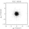 |
Fig. 3 Proper motion distribution for stars belonging to the globular cluster NGC 6656 observed in Field 10-8. |
Thus, our results confirm the reliability of our proper motion technique and in addition, match the precision achieved by our bulge radial velocities measurements in our three off-axis fields (~30 km s-1), which are included in a separate paper (Soto et al. 2012).
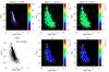 |
Fig. 4 Binned CMDs for NGC 6656 stars in Field 10-8 (l,b) = (2.91°, − 7.96°) with nfit ≥ 6. The stars have been selected kinematically using the small kinematic dispersion of the cluster proper motions. The parameter nfit corresponds to the minimum number of exposures fitted by the proper motion solution of each star. Some plots have been color-coded using the proper motions and derived dispersions. Top row, left to right: stellar density, mean longitudinal proper motion, mean latitudinal proper motions. Bottom, left to right: unbinned CMD, longitudinal dispersion in proper motions, latitudinal dispersion in proper motions. |
Proper motion dispersions in NGC 6656.
Proper motion dispersions.
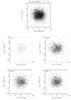 |
Fig. 5 Top row: proper motion distribution for WFPC2 in Field 4-7. Second and third rows: proper motion distribution on individual CCD frames of WFPC2, Planetary Camera (PC), and Wide Field Camera 2 (WF2), Wide Field 3 (WF3) and Wide Field 4 (WF4). |
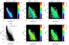 |
Fig. 8 Binned CMDs of Field 4-7 field (l,b) = (3.58°, − 7.17°) with nfit ≥ 6. The unbinned CMD is the only plot in this figure including all the stars with available photometry regardless of the respective nfit for clarity. |
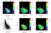 |
Fig. 9 Binned CMDs of Field 3-8 field (l,b) = (2.91°, − 7.96°) with nfit ≥ 5. |
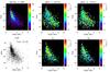 |
Fig. 10 Binned CMDs of Field 10-8 field (l,b) = (9.86°, − 7.61°) with nfit ≥ 6. |
4. Analysis
Our proper motion results are plotted in Figs. 5–7; the proper motion dispersions, and numbers per field are given in Table 3, where the terms of the velocity ellipsoid tensor (Zhao et al. 1994) are defined by  (1)Color–magnitude diagrams for the three fields color-coded by the proper motion information are shown in Figs. 8–10. The first indication of the correct performance of our procedures appears in Table 3 in that there is no evidence of significant variations or inconsistencies in the kinematics between the stars in the WF and PC chips. Similarly, we find that the proper motion distributions do not differ dramatically from one field to the other. This agreement in the proper-motion distribution seems to even extend to the fields presented in KR02 close to the Galactic minor axis (see Table 4).
The three fields in the present study, all of which are at positive Galactic longitudes, have distributions with no significant correlation rlb between l and b proper motions; at the same time, σl and σb are slightly larger than the dispersions found in minor axis fields in KR02. Zoccali et al. (2008) found a decreasing dispersion of radial velocities when moving away from the disk for a bulge population close to the minor axis. A similar result was found by Soto et al. (2012) in their minor axis fields, consistently. This gradient is not observed in the radial velocities of the same off-axis fields analyzed in this work. There are two possible reasons for an increase in σl and σb. It either may be that the increase in dispersion is due to a higher contamination by foreground disk populations, thereby decreasing the total number of bulge stars detected or that there is a real, intrinsic increase in the dispersions due to the location of the fields in the sky (e.g., compared with the minor axis fields, we might be sampling different bulge orbit families or the same orbits at a different bulge location in this off-axis fields). Below we try to discern which of these effects prevail using the assistance of the CMD information.
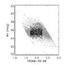 |
Fig. 11 Photometric parallax M* as a function of the color for a subsample of main-sequence stars in Field 4-7. Black dots have been used to derive the respective photometric distance D*. |
The binned CMDs (Figs. 8–10) for the three fields show some distinctive features. First, there is a cut-off at the bright end of the CMDs because of saturation in the first-epoch long exposures (>1200 s). This saturation limit, in turn, limited our proper motions to main sequence (MS) stars below the turn-off. In contrast, the fields in KR02 had many shorter exposures in their first epoch, allowing them to reach both the turn-off and red-giant branch (RGB). A second feature hinted in the three fields is a gradient perpendicular to the main sequence in the mean μl. Such a gradient, which for a given color shows a drift toward negative μl, has been clearly observed in the Galactic minor-axis fields in KR02. In our fields, however, the appearance is noisier, which is likely due to the reduced statistics. The gradient can be explained as a signature of the rotation through the galaxy, where high positive μl should correspond mainly to the foreground population rotating in front of the bulge. We explore the significance of this gradient later in this section in more detail. Interestingly, a similar but noisier feature appears in the mean μb panels. This might be caused by a combination of the projection effect of the bulge orbits and the contamination by the disk.
We explore these effects further on Field 4-7, which consists of a higher number of proper motions compared with Field 3-8 and Field 10-8, and therefore allows a more robust analysis. We followed a similar procedure to dissect the stellar populations in our fields than KR02 and K04. We have chosen a crude distance modulus as an indicator of the distances toward the Galactic bulge. The quantity M* can be defined as  (2)and has been used to remove the slope of the main sequence stars in the CMD for our proper motion sample. The coefficient of three for the color, as opposed to two in KR02, is due to the use of F606W-F814W, as opposed to F555W-F814W.
Thus, the proper motions as a function of this distance modulus, M*, can be explored. Figure 11 shows the distance modulus M* as a function of the color for a subsample of main-sequence stars, while Fig. 12 shows the proper motion means and dispersions, as a function of M* for Field 4-7. Again, this field was chosen for its better statistics as compared to the number of stars with proper motions in the two other fields, Field 3-8 and Field 10-8. The mean μl motion again shows the kinematic feature previously observed in Fig. 8, which we relate to the rotation of stars across the Galactic bulge. In addition, Field 4-7 proper motion dispersions σl show a mild trend for closer main sequence stars to have comparatively higher values than main sequence stars lying farther away. This can be interpreted as a distance effect, and it is also a nice demonstration that noise does not dominate our results.
Figure 13 illustrates the photometric distance D* (left panel), derived from M*, as a function of the color. The right panel shows the angle φlb as a function of distance, D*. Here, φlb is the equivalent to the vertex angle, but in the l-b velocity plane, and D* has been binned for clarity. In order to obtain completeness in distance reaching our last bin (D* ~ 20 kpc), a narrower region in D* was selected from the initial main sequence subsample. The selection is based on the one performed in K04 for the field near NGC 6558, and is shown by the black points in the Fig. 11 and the left panel of the Fig. 13. The angle φlb has been calculated using an iterative clipping algorithm that rejects stars beyond 3σ of the distribution to avoid contamination. In addition, the Spearman correlation coefficient, rS, is calculated in each case from the same stars in the first iteration of the velocity ellipsoid calculation, in order to have an independent measurement of the correlation between μl and μb. Errors in φlb and rS come from bootstrap Montecarlo realizations, and the error bars are indicated in the Fig. 14.
Figure 14 and Table 5 show the velocity ellipsoids and respective φlb and rS for Field 4-7. These parameters clearly show a change in the orientation of the velocity ellipsoid. Clarkson et al. (2008) also find significant changes in the orientation of the l,b velocity ellipsoid in their improved sample of ACS proper motions in Sagittarius-I. This orientation changes in the velocity ellipsoid are difficult to interpret, especially at different longitudes, owing to projection effects, and will be addressed in the future using our dynamical models.
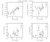 |
Fig. 12 Mean proper motions and dispersions as a function of the photometric parallax M*, for the subsample of main sequence stars in Field 4-7, where each point corresponds to 180 stars. The higher number of stars on this field has allowed us to explore the proper motions as a function of M*. The rotation pattern speed clearly appears on this field for μl (top left). Similarly, σl (bottom left) also indicates a decreasing dispersion for stars lying farther away, as expected when observing the Galactic rotation. |
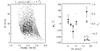 |
Fig. 13 Left, distance D*, derived from M*, as a function of the color in Field 4-7. Right, angle φlb as a function of binned D*, equal numbers of stars have been selected per bin; in addition, the Spearman correlation coefficient rS has been calculated in each bin to have a independent correlation measurement between l and b. |
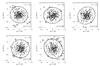 |
Fig. 14 Velocity ellipsoids used to calculate the angle φlb in Field 4-7. An iterative clipping algorithm has been used to exclude stars beyond 3σ. Stars rejected during the process are enclosed by squares. |
φlb and Spearman correlation coefficients rS at different distance bins for Field 4-7.
5. Conclusions
We have presented ~15 000 new proper motions for three off-axis fields of the Galactic bulge. The results for these three fields show remarkable agreement with the results in KR02, and thus suggests a bulge structure where the kinematics observed close to the center along the Galactic minor axis are repeated to some extent in higher longitudes. Despite the reduced number of proper motions in comparison with minor axis fields, the rotation of the bulge is still visible in our fields, which reach l ~ 10°. We explored the possible changes in the velocity (proper motion) ellipsoid within Field 4-7 as a function of the distance along the line of sight; as is the case with the results of Clarkson et al. (2008), we found a change in the tilt of the { l,b } velocity ellipsoid.
All of this suggests that a significant fraction of the population follows bulge-like orbits, even at the location of our three off-axis fields in the outer bulge. If we consider the anisotropies produced by the bar in the minor-axis (inner bulge) fields, what we observe should therefore be part of the Galactic bar. The importance of the extent of the bar can be related to the evolutionary stage of the bulge, where slow-rotating long bars can evolve from rapid-rotating short bars secularly (e.g. Combes 2007; Athanassoula 2005), thus this information can provide important constraints on the bulge structure and formation. Dynamical models including this new proper motion data will be able to provide new insight into the actual bulge structure, until now poorly constrained.
Finally, we have demonstrated the technical feasibility of proper-motion measurements using different cameras with different geometries for the first and second epochs. Field 10-8 with its globular cluster NGC 6656 has provided us with a direct assessment of the accuracy of our proper motion procedure. A cluster dispersion of ~0.9 mas yr-1 or ~14 km s-1 at 3.2 kpc supports our claim of ~30 km s-1 accuracy for bulge stars. Unfortunately, our results are severely affected by the saturation of the long first-epoch exposures, and could be significantly improved by a third ACS epoch.
Acknowledgments
M.S. acknowledges support by Fondecyt project 3110188 and Comité Mixto ESO- Chile. R.M.R. acknowledges funding from GO-9816 and from AST-0709479 from the National Science Foundation. This material is based upon work supported in part by the National Science Foundation under Grant No. 1066293 and by the hospitality of the Aspen Center for Physics.
References
- Anderson, J., & King, I. R. 1999, PASP, 111, 1095 [NASA ADS] [CrossRef] [Google Scholar]
- Anderson, J., & King, I. R. 2000, PASP, 112, 1360 [NASA ADS] [CrossRef] [Google Scholar]
- Anderson, J., & King, I. R. 2002, ASPC, 273, 167 [NASA ADS] [Google Scholar]
- Anderson, J., & King, I. R. 2003, AJ, 126, 772 [NASA ADS] [CrossRef] [Google Scholar]
- Anderson, J., & King, I. R. 2006, Instrument Science Report ACS 2006-01 (Batimore: STScI) [Google Scholar]
- Athanassoula, E. 2005, MNRAS, 358, 1477 [NASA ADS] [CrossRef] [Google Scholar]
- Babusiaux, C., Gómez, A., Hill, V., et al. 2010, A&A, 519, A77 [NASA ADS] [CrossRef] [EDP Sciences] [Google Scholar]
- Ballero, S. K., Matteucci, F., Origlia, L., & Rich, R. M. 2007, A&A, 467, 123 [Google Scholar]
- Benjamin, R. A., Churchwell, E., Babler, B. L., et al. 2005, ApJ, 630, L149 [NASA ADS] [CrossRef] [Google Scholar]
- Bensby, T., Adn, D., Melndez, J., et al. 2011, A&A, 533, A134 [NASA ADS] [CrossRef] [EDP Sciences] [Google Scholar]
- Binney, J., Gerhard, O. E., Stark, A. A., Bally, J., & Uchida, K. I. 1991, MNRAS, 252, 210 [NASA ADS] [CrossRef] [Google Scholar]
- Chen, D., Chen, L., & Wang, J.-J. 2004, Chinese Physics Letters, 21, 1673 [NASA ADS] [CrossRef] [Google Scholar]
- Clarkson, W., Sahu, K., Anderson, J., et al. 2008, ApJ, 684, 1110 [NASA ADS] [CrossRef] [Google Scholar]
- Combes, F. 2007, IAUS, 235, 19 [NASA ADS] [Google Scholar]
- Cudworth, K. M. 1986, AJ, 92, 348 [NASA ADS] [CrossRef] [Google Scholar]
- Dolphin, A. 2000, PASP, 112, 1397 [NASA ADS] [CrossRef] [Google Scholar]
- Dwek, E., Arendt, R. G., Hauser, M. G., et al. 1995, ApJ, 445, 716 [CrossRef] [Google Scholar]
- Englmaier, P., & Gerhard, O. 1999, MNRAS, 304, 512 [NASA ADS] [CrossRef] [Google Scholar]
- Feltzing, S., & Gilmore, G. 2000, A&A, 355, 949 [NASA ADS] [Google Scholar]
- Fulbright, J. P., McWilliam, A., & Rich, R. M. 2007, ApJ, 661, 1152 [NASA ADS] [CrossRef] [Google Scholar]
- Harris, W. E. 1996, AJ, 112, 1487 [NASA ADS] [CrossRef] [Google Scholar]
- Hill, V., Lecureur, A., Gomez, A., et al. 2011, A&A, 534, A80 [NASA ADS] [CrossRef] [EDP Sciences] [Google Scholar]
- Holtzman, J. A., Watson, A. M., Baum, W. A., et al. 1998, AJ, 115, 1946 [NASA ADS] [CrossRef] [Google Scholar]
- Kozhurina-Platais, V., Goudfrooij, P., & Puzia, T. H. 2007, Instrument Science Report ACS 2007-04 (Batimore: STScI) [Google Scholar]
- Kozłowski, S., Woźniak, P. R., Mao, S., et al. 2006, MNRAS, 370, 435 [NASA ADS] [CrossRef] [Google Scholar]
- Kuijken, K. 2004, ASP, 317, 310K (K04) [NASA ADS] [Google Scholar]
- Kuijken, K., & Merrifield, M. R. 1995, ApJ, 443, L13 [NASA ADS] [CrossRef] [Google Scholar]
- Kuijken, K., & Rich, R. M. 2002, AJ, 124, 2054 (KR02) [NASA ADS] [CrossRef] [Google Scholar]
- McWilliam, A., & Rich, R. M. 1994, ApJS, 91, 749 [NASA ADS] [CrossRef] [Google Scholar]
- Minniti, D. 1993, IAU Symp., 153, 315 [NASA ADS] [Google Scholar]
- Minniti, D. 1996, ApJ, 459, 175 [NASA ADS] [CrossRef] [Google Scholar]
- Peterson, R. C., & Cudworth, K. M. 1994, ApJ, 420, 612 [NASA ADS] [CrossRef] [Google Scholar]
- Rattenbury, N. J., Mao, S., Debattista, V. P., et al. 2007a, MNRAS, 378, 1165 [NASA ADS] [CrossRef] [Google Scholar]
- Rattenbury, N. J., Mao, S., Sumi, T., & Smith, M. C. 2007b, MNRAS, 378, 1064 [NASA ADS] [CrossRef] [Google Scholar]
- Rich, R. M. 1988, AJ, 95, 828 [NASA ADS] [CrossRef] [Google Scholar]
- Rich, R. M. 1990, ApJ, 362, 604 [NASA ADS] [CrossRef] [Google Scholar]
- Rich, R. M., Reitzel, D. B., Howard, C. D., & Zhao, H. 2007, ApJ, 658, L29 [NASA ADS] [CrossRef] [Google Scholar]
- Sadler, E. M., Rich, R. M., & Terndrup, D. M. 1996, AJ, 112, 171 [NASA ADS] [CrossRef] [Google Scholar]
- Saha, K., Martinez-Valpuesta, I., & Gerhard, O. 2012, MNRAS, 421, 333 [NASA ADS] [Google Scholar]
- Samus, N., Kravtsov, V., Pavlov, M., Alcaino, G., & Liller, W. 1995, A&AS, 109, 487 [NASA ADS] [Google Scholar]
- Schwarzschild, M. 1979, ApJ, 232, 236 [NASA ADS] [CrossRef] [Google Scholar]
- Schwarzschild, M. 1982, ApJ, 263, 599 [NASA ADS] [CrossRef] [Google Scholar]
- Shen, J., Rich, R. M., Kormendy, J., et al. 2010, ApJ, 720, 72 [Google Scholar]
- Soto, M. 2010, Ph.D. Thesis, Leiden Observatory, The Netherlands [Google Scholar]
- Soto, M., Rich, R. M., & Kuijken, K. 2007, ApJ, 665, L31 [NASA ADS] [CrossRef] [Google Scholar]
- Soto, M., Kuijken, K., & Rich, R. M. 2012, A&A, 540, A48 [NASA ADS] [CrossRef] [EDP Sciences] [Google Scholar]
- Spaenhauer, A., Jones, B. F., & Withford, E. 1992, AJ, 103, 297 [NASA ADS] [CrossRef] [Google Scholar]
- Sumi, T., Wu, X., Udalski, A., et al. 2004, MNRAS, 348, 1439 [NASA ADS] [CrossRef] [Google Scholar]
- Terndrup, D. M., Rich, R. M., & Sadler, E. M. 1995, AJ, 110, 1774 [NASA ADS] [CrossRef] [Google Scholar]
- Tonry, J., & Davis, M. 1979, AJ, 84, 10 [Google Scholar]
- Vieira, K., Casetti-Dinescu, D. I., Méndez, R. A., et al. 2007, AJ, 134, 1432 [NASA ADS] [CrossRef] [Google Scholar]
- Zhao, H. S. 1996, MNRAS, 283, 149 [NASA ADS] [CrossRef] [Google Scholar]
- Zhao, H. S., Spergel, D. N., & Rich, R. M. 1994, AJ, 108, 2154 [NASA ADS] [CrossRef] [Google Scholar]
- Zhao, H. S., Rich, R. M., & Spergel, D. N. 1996, MNRAS, 282, 175 [NASA ADS] [CrossRef] [Google Scholar]
- Zoccali, M., Lecureur, A., Barbuy, B., et al. 2006, A&A, 457, L1 [NASA ADS] [CrossRef] [EDP Sciences] [Google Scholar]
- Zoccali, M., Hill, V., Lecureur, A., et al. 2008, 486, 177 [Google Scholar]
All Tables
φlb and Spearman correlation coefficients rS at different distance bins for Field 4-7.
All Figures
|
Fig. 1 The rms residuals of the pixels positions in x (bottom) and y (top) from the proper motion fits in one of our fields, Field 4-7 WF2. The solid lines are the best theoretical fit for an error estimation based on photon noise alone (bottom line) and for photon noise including additional systematic source of errors for each epoch (top two lines). This plot shows that the dominant source of error for the fainter undithered first epoch (red) is photon noise, while for brighter sources a residual systematic error appears that we relate to saturation due to the long exposures. Second-epoch dithered exposures (green) are best represented by a systematic error that has been included in the estimation of the proper motion error. |
| In the text | |
|
Fig. 2 Kinematic selection of cluster stars in Field 10-8 in one of the cameras of WFPC2, Wide Field 4 (WF4). The selection was performed for each chip separately using a hard cut-off; cluster stars have a small velocity dispersion, which therefore biases the relative zeropoint of the proper motions of bulge stars. Thus, the cluster stars must be excluded from the reference frame used to calculate bulge proper motions. Top panel: proper motions in pixel yr-1 before the refinement of the stars used as the basis for the inter-epoch transformations for WF4 chip in Field 10-8; where black dots are bulge stars, and orange dots are those kinematically classified as cluster stars. Second row: proper motions in pixels μx and μy as a function of the x − y coordinates before the correction. Bottom row: same as the second row, but after applying the correction. |
| In the text | |
|
Fig. 3 Proper motion distribution for stars belonging to the globular cluster NGC 6656 observed in Field 10-8. |
| In the text | |
|
Fig. 4 Binned CMDs for NGC 6656 stars in Field 10-8 (l,b) = (2.91°, − 7.96°) with nfit ≥ 6. The stars have been selected kinematically using the small kinematic dispersion of the cluster proper motions. The parameter nfit corresponds to the minimum number of exposures fitted by the proper motion solution of each star. Some plots have been color-coded using the proper motions and derived dispersions. Top row, left to right: stellar density, mean longitudinal proper motion, mean latitudinal proper motions. Bottom, left to right: unbinned CMD, longitudinal dispersion in proper motions, latitudinal dispersion in proper motions. |
| In the text | |
|
Fig. 5 Top row: proper motion distribution for WFPC2 in Field 4-7. Second and third rows: proper motion distribution on individual CCD frames of WFPC2, Planetary Camera (PC), and Wide Field Camera 2 (WF2), Wide Field 3 (WF3) and Wide Field 4 (WF4). |
| In the text | |
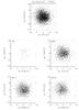 |
Fig. 6 Same as Fig. 5, but for Field 3-8. |
| In the text | |
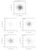 |
Fig. 7 Same as Fig. 5, but for Field 10-8. |
| In the text | |
|
Fig. 8 Binned CMDs of Field 4-7 field (l,b) = (3.58°, − 7.17°) with nfit ≥ 6. The unbinned CMD is the only plot in this figure including all the stars with available photometry regardless of the respective nfit for clarity. |
| In the text | |
|
Fig. 9 Binned CMDs of Field 3-8 field (l,b) = (2.91°, − 7.96°) with nfit ≥ 5. |
| In the text | |
|
Fig. 10 Binned CMDs of Field 10-8 field (l,b) = (9.86°, − 7.61°) with nfit ≥ 6. |
| In the text | |
|
Fig. 11 Photometric parallax M* as a function of the color for a subsample of main-sequence stars in Field 4-7. Black dots have been used to derive the respective photometric distance D*. |
| In the text | |
|
Fig. 12 Mean proper motions and dispersions as a function of the photometric parallax M*, for the subsample of main sequence stars in Field 4-7, where each point corresponds to 180 stars. The higher number of stars on this field has allowed us to explore the proper motions as a function of M*. The rotation pattern speed clearly appears on this field for μl (top left). Similarly, σl (bottom left) also indicates a decreasing dispersion for stars lying farther away, as expected when observing the Galactic rotation. |
| In the text | |
|
Fig. 13 Left, distance D*, derived from M*, as a function of the color in Field 4-7. Right, angle φlb as a function of binned D*, equal numbers of stars have been selected per bin; in addition, the Spearman correlation coefficient rS has been calculated in each bin to have a independent correlation measurement between l and b. |
| In the text | |
|
Fig. 14 Velocity ellipsoids used to calculate the angle φlb in Field 4-7. An iterative clipping algorithm has been used to exclude stars beyond 3σ. Stars rejected during the process are enclosed by squares. |
| In the text | |
Current usage metrics show cumulative count of Article Views (full-text article views including HTML views, PDF and ePub downloads, according to the available data) and Abstracts Views on Vision4Press platform.
Data correspond to usage on the plateform after 2015. The current usage metrics is available 48-96 hours after online publication and is updated daily on week days.
Initial download of the metrics may take a while.