| Issue |
A&A
Volume 561, January 2014
|
|
|---|---|---|
| Article Number | A111 | |
| Number of page(s) | 9 | |
| Section | Catalogs and data | |
| DOI | https://doi.org/10.1051/0004-6361/201322924 | |
| Published online | 16 January 2014 | |
U-band photometry of 17 WINGS clusters⋆
1 Specola Vaticana, 00120, Vatican City State
e-mail:
This email address is being protected from spambots. You need JavaScript enabled to view it.
2
INAF – Padova Astronomical Observatory,
Vicolo Osservatorio
5, 35122
Padova,
Italy
3 GRANTECAN S.A., Centro de Astrofísica de La Palma, C/Cuesta
de San José s/n, 38712 Breña Baja ( La Palma), Spain
4
INFN, Sezione di Roma, Tor Vergata, 00133
Rome,
Italy
5
Department of Physics, University of Rome,
Tor Vergata, 00133
Rome,
Italy
6
INAF – Napoli Astronomical Observatory,
Salita Molariello
16, 80131
Napoli,
Italy
7
Department of Physics and Astronomy, Vicolo Osservatorio 2, 35122
Padova,
Italy
8
Centro de Estudios de Física del Cosmos de Aragón (CEFCA), Plaza
San Juan 1, planta 2, 44001
Teruel,
Spain
9
Sterrekundig Observatorium Vakgroep Fysica en Sterrekunde
Universiteit Gent, Krijgslaan
281-S9, 9000
Gent,
Belgium
10
Observatoire de Genève, Université de Genève,
51 Ch. des
Maillettes, 1290
Versoix,
Switzerland
11
INAF – Roma Astronomical Observatory, 00040
Monteporzio,
Italy
Received: 28 October 2013
Accepted: 25 November 2013
Abstract
Context. This paper belongs to a series presenting the WIde Field Nearby Galaxy-cluster Survey (WINGS). The WINGS project has collected wide-field, optical (B, V), and near-infrared (J, K) imaging as well as medium resolution spectroscopy of galaxies in a sample of 76 X-ray selected nearby clusters (0.04 <z< 0.07) with the aim of establishing a reference sample for evolutionary studies of galaxies and galaxy clusters.
Aims. We present the U-band photometry of galaxies and stars in the fields of 17 clusters of the WINGS sample. We also extend the original B- and V-band photometry (WINGS-OPT) for 9 and 6 WINGS clusters to a larger field of view.
Methods. We used both the new and already existing B-band photometry to obtain reliable (U − B) colors of galaxies within three fixed apertures in kpc. To this aim, we took particular care with the astrometric precision in the reduction procedure. Since not all the observations were taken in good transparency conditions, the photometric calibration was partly obtained by relying on the SDSS and WINGS-OPT photometry for the U- and optical bands, respectively.
Results. We provide U-band (also B- and V-band, where possible) total magnitudes of stars and galaxies in the fields of clusters. For galaxies only, the catalogs also provide geometrical parameters and carefully centered aperture magnitudes. The internal consistency of magnitudes was checked for clusters imaged with different cameras, while the external photometric consistency was obtained by comparison with the WINGS-OPT and SDSS surveys.
Conclusions. The photometric catalogs presented here add the U-band information to the WINGS database for extending the spectral energy distribution of the galaxies, in particular in the ultraviolet wavelengths which are fundamental for deriving the star formation rate properties.
Key words: galaxies: clusters: general / galaxies: photometry / catalogs
Photometric catalogs are only available at the CDS via anonymous ftp to cdsarc.u-strasbg.fr (130.79.128.5) or via http://cdsarc.u-strasbg.fr/viz-bin/qcat?J/A+A/561/A111
© ESO, 2014
1. Introduction
In the current standard cosmological paradigm, clusters accrete individual galaxies and larger subclumps from their outskirts. In this scenario, the infalling regions of clusters are naturally very important, which are the transition regions in which galaxies are subject to a dramatic change of environment, because they feel the effects of the high-density environment for the first time. A morphological transformation of spirals into S0 galaxies appears to occur in clusters at z> 0.2, most likely driven by environmental effects (Dressler et al. 1997; Fasano et al. 2000). The environment also appears to have a strong influence on the star formation activity (SFA) of disk galaxies in clusters at high redshift, apparently suppressing it upon infall into rich clusters (Balogh et al. 1997; Couch et al. 1998, 2001; Dressler et al. 1999; Poggianti et al. 1999). Indeed, observations probing the star formation, Hubble types, and gas content of galaxies in clusters have proved that the cluster outskirts are essential for understanding galaxy transformations (Abraham et al. 1996; Balogh et al. 1997; Ellingson et al. 2001; Solanes et al. 2001; Pimbblet et al. 2002; Treu et al. 2003; Kodama et al. 2001, 2004; McIntosh et al. 2004). In particular, several recent works have shown that in the local Universe the correlation between SFA and local density extends to very large clustercentric radii, well beyond the cluster central regions (Lewis et al. 2002; Gomez et al. 2003; Balogh et al. 1997). The assembly of clusters, by itself, seems to be able to suppress the star formation, as suggested by the detection of post-starburst galaxies at the interface of cluster infalling substructures (Poggianti et al. 2004).
In the past years many high-quality (HST) observations have been devoted to the study of clusters at intermediate and high redshift, while for the local volume, Virgo, Fornax and Coma clusters constituted the main reference sample until a few years ago. To fill in this gap, we started the WIde Field Nearby Galaxy-cluster Survey (WINGS, Fasano et al. 2006, hereafter Paper I). This survey has focused on clusters located in the redshift range 0.04−0.07 and has collected wide-field optical (B,V) imaging (Varela et al. 2009, WINGS-OPT) for a sample of 76 clusters selected from three X-ray flux-limited samples compiled from the ROSAT All-Sky Survey (Ebeling et al. 1996, 1998, 2000). In addition, multifiber, medium-resolution spectroscopy and near-infrared (J,K), wide-field imaging has been obtained for 48 and 28 WINGS clusters (Cava et al. 2009; Valentinuzzi et al. 2009).
To complement the WINGS database with U-band imaging, we gathered observations for a subsample of 17 WINGS clusters using three different telescopes equipped with different wide-field cameras and a few archival data.
These observations allow one to study in detail the SFA in a statistically significant sample of cluster galaxies. Because the integrated spectrum of a galaxy is increasingly dominated by young stars with shorter wavelengths, U-band data is by far more sensitive to any current or recent star formation than any of the other broadbands available (Kennicutt 1998; Barbaro & Poggianti 1997). Our U-band estimates of the current star formation are truly integrated values (though dustaffected), and can be compared with the estimates based on our optical spectroscopy, which samples only the very central regions of each galaxy (1.6″/2.6″). Moreover, the spatial distribution of the U-band emission within galaxies greatly helps in distinguishing between the various physical processes, by revealing whether star formation is preferentially suppressed and/or enhanced in the central and outskirt regions of galaxies. In particular, the distribution of the SFA in galaxies residing in the cluster outskirts (infalling region) might reveal whether they are affected by ram pressure stripping (SFA in the outer regions), by shock-induced star formation related to the galaxy infalling into the cluster (SFA on the impact edge of the galaxies), or by centrally driven starbursts due to tidal repeated encounters in the cluster potential (SFA in the nuclear regions). Moreover, these observations are expected to allow us to establish how the SFA correlates with galaxy morphology (from the V-band imaging), mass (from K-band data) and spectra, as well as with the environment (local density and cluster properties).
The paper is organized as follows: Sect. 2 describes our observations and data reduction. In Sect. 3 we present the catalogs, and in Sect. 4 the data quality is analyzed. Throughout the paper we use the following cosmology: H0 = 70 km s-1 Mpc-1, Ωm = 0.3 and ΩΛ = 0.7. The magnitudes are given in the Vega system.
2. Observations and data reduction
The data presented in this paper are based on observations obtained with three different wide-field cameras (see Table 1): (i) the 90prime camera at the 90-inches BOK telescope (90prime (BOK), Kitt Peak); (ii) the Wide Field Camera at the 2.5 m Isaac Newton Telescope (INT/WFC); (iii) the Large Binocular Camera at the Large Binocular Telescope (LBT/LBC). For one cluster (Abell 970) we used imaging data from the MPG/WFI (ESO 2.2 archive). All clusters have been imaged in the U-band. Many clusters have also been imaged in the optical (B,V) bands.
The cameras.
The runs.
In Table 2 we report the observing log, one row per run (per night in the case of the LBC observations), each row including the number of imaged clusters. In Table 3 the list of the observed clusters is reported. In addition the average coordinates and redshifts of the clusters, we list the telescopes used to image each cluster in Col. 5. The BOK observations always include the U-, B-, and V-bands, while the INT and MPG observations just include the U-band. For the clusters imaged with LBT, we list in parenthesis the filters used for the imaging. The full widths at half maximum (FWHMs) for each cluster in each filter are given in the headers of the catalogs (see the first group of rows of the header in Fig. 1). With the WFC, 90prime, and LBC cameras we imaged eight, six, and six clusters, respectively. Some clusters were observed with two or three instruments for a total of 15 clusters observed in the U-band. To these observations we added U-band imaging of the cluster Abell 970, taken from the MPG/WFI (ESO 2.2 archive). The data sets coming from the four instruments (WFC, 90prime, LBC, and WFI) span a time interval of about four years and reflect different proposal strategies (observing constraints and requirements), also depending on the available observing time. Therefore, because of the quite heterogeneous instrument sets and weather conditions, we used different reduction strategies for the different cameras, as outlined in the following subsections.
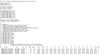 |
Fig. 1 Header and first rows of the catalog from BOK imaging of A1795. |
The observed clusters.
2.1. INT observations
We obtained INT/WFC imaging of nine clusters during three useable nights of the same observing run (May 10/12/13 2005). For the outline of the camera we refer to Table 1 and Paper I. The observations have been taken, under generally good weather conditions, just in the U-band and trying to match the field of view of the B- and V-band imaging already available in the WINGS-OPT survey as closely as possible. To cover the gaps between the CCDs, at least three 20 min dithered exposures per cluster were acquired. During each night standard field exposures were secured to allow photometric calibration.
Bias subtraction and flat-field corrections were separately performed on each of the four CCDs of the WFC, while the mosaic-image of each exposure was produced using the IRAF tool wfcmosaic. The mean error of the astrometric solution, obtained for every exposure from the USNO star catalog, was ≤0.3 arcsec (~1 pixel) over the field. The final image of each cluster was obtained by weighted mean combination of the dithered exposures.
During the run, the system proved to be very stable, while the photometric calibration showed that the transparency did not change significantly. The cluster A1991 was excluded from the final INT sample since the outlined reduction procedure was not able to repair some temporary failure of the acquisition system, which causes disparity among the CCDs.
2.2. BOK observations
The 90prime camera mounted at the BOK telescope (Kitt Peak) during our 2006 observing runs was a mosaic of four CCDs separated in two directions by very large inter-CCD gaps (about 15.76 mm or 1050 pixels). The edge-to-edge field of view, including the inter-CCD gaps, was 1.16 × 1.16 degrees, with a plate scale of 30.2′′/mm or 0.45′′/pixel.
In five nights, sharing two observing runs (see Table 2 for details), we imaged eight clusters in the U-, B-, and V-band. To fill the large gaps between the CCDs, we shifted the telescope to five different positions, thus covering the entire field of view of the camera.
During each night, dome and twilight sky flats were obtained and several photometric standard fields were imaged in each photometric band and at different zenithal distances. Unfortunately, in both observing runs the weather conditions were inclement. In particular, the average seeing was about 2′′ and the sky transparency was not good.
Owing to the very large angular view provided by the 90prime camera, we were forced to adopt a more laborious procedure than for the INT data reduction, to obtain a good enough astrometry over the whole field. In particular, relying on the stars of the USNO catalog in a suitable (filter-dependent) magnitude range, we first obtained for each filter and for each CCD an average astrometric solution relative to the geometrical center of the camera, stacking all the mosaic images obtained in that filter. Then, using 15 stars for each CCD (three in every corner and three in the center), we improved the astrometic solution of each CCD for each exposition and translated it into the proper position on the sky. The rms of the angular distances between the BOK and USNO coordinates was less than 0.25 arcsec.
To obtain the final mosaic for every field, we used SWARP (Bertin & Arnouts 1996) by Terapix. Using our astrometric projection defined in the WCS standard, SWARP resampled and co-added the set of five dithered exposures for each cluster in each filter, thus producing the final, backgroud-subtracted image. Two of the eight imaged clusters (A2256 and RX0058) were observed under quite poor weather conditions. They were excluded from the final BOK sample.
Even though the standard field exposures were as diligently processed as for the scientific ones, they were only used to obtain the relative photometric calibration within the 90prime field, that is to estimate possible gain and linearity differences among the CCDs. In fact, because of the poor transparency, we were forced in both runs to perform the absolute photometric calibration (zero points and color terms) relying on the WINGS-OPT catalogs (Varela et al. 2009, for the V- and B-band) and on the Sloan Digital Sky Survey DR7 photometric data (Abazajian et al. 2009), suitably converted in to the Johnson system (Lupton 2005, for the U-band).
2.3. LBT observations
The LBC FITS images are multi extension files (MEF) composed of a mosaic of four CCDs of 4608 × 2048 pixels with a median plate scale of 0.225′′/pixels and a scientific field of view (FoV) of about 23.6 × 25.3 arcmin2. Therefore, to cover the field imaged by the WINGS-OPT survey, five exposures per cluster were planned.
The observations of our clusters have been taken in service mode during science demonstration time (SDT) under variable transparency and seeing conditions. The data set resulting from these circumstances was not optimal, since in many cases the cluster field coverage was incomplete (sometimes sparse), or the different exposures of the same cluster were taken in different seeing and transparency conditions. Finally, only six clusters had enough field coverage and seeing homogeneity to be included in the final LBT sample. Three of them were imaged in both U- and B-band, while for two clusters only U-band imaging was available. Finally, for RX1740 we only obtained B-band imaging.
The reduction was performed by one of us (CD) using the standard procedure devised by the LBC Team1. In most CCD mosaic imagers, electronic ghosts are present due to video channel cross-talk, and a specifically designed software procedure (xtalk) was used to remove these features; for LBC the cross talk coefficient is about 3.0E-05.
The flat-field images were derived from twilight-sky data and a calibration master-flat was obtained by stacking a set of flat images with a sigma-clipping rejection algorithm with radial profile normalized to unity in the center. The saturated pixels, poor-signature chips, cosmic-ray events, and satellite trails were masked using a dedicated derivative algorithms developed by the LBC team.
The area of the LBC pixels is not constant over the entire field of view (FoV), because of the effect of astrometric distortions (also called sky concentration). To correct for this feature and normalize the pixel area, a sky-concentration image was applied as multiplicative factor. This filter-dependent correction image was produced by a dedicated software that uses as input information the astrometric solution for the specific filter. After this correction, it was possible to mask all objects in the image and stack all frames within a fixed temporal window (about 10 min) to allow a proper subtraction of the small-scale features of the background. This temporal window is representative of the main sky-background variation and features such as fringes. For the U- and B-band this procedure produced well-flattened images and no additional processing was required.
The background-subtracted images were corrected for object photometry altered by sky-concentration effects dividing by the same correction image as used in the previous reduction step. In fact, the sky concentration effects modify the surface brightness of the background, producing a typical pin-cushion feature, but this does not alter the integrated flux of extended objects. Therefore, each science image must first be multiplied by the sky-concentration image to rectify the background, and after it is properly subtracted, it must be divided by the same sky-concentration image to correct the flux of stars and galaxies to their original value. Because it is a prime focus camera, the optical distortions of LBC are quite significant. Still, after the procedure outlined above, the quality of the point spread function (PSF) over the entire LBC FoV was independent of the radial distance from the optical center.
The astrometric solution was computed through a three-pass process by the AstromC package (Radovich et al. 2004): 1) the offsets of the four chips were computed by matching a catalog of objects found on the frame with an astrometric catalog (usually USNOA B1.0 catalog); 2) an overall fit was performed to obtain a local chip-to-chip astrometric solution by applying the calculated deformation map obtained with Stone (1997) astrometric fields (and UCAC catalogs), as described in Giallongo et al. (2008, G08 hereafter); 3) the final astrometric solution was computed on the whole dithered image set, thus providing a well-minimized global fit.
Since no photometric standard fields were imaged during the SDT runs, the (provisional) photometric calibration was obtained using the coefficients given in Table 2 of G08. These coefficients are the result of several commissioning nights devoted only to the photometric characterization of the LBC at the LBT. The nominal photometric accuracy in the overall field is about of 0.01 mag. We refer to G08 for more details about the LBC instrument and the data reduction procedures. The final zero points were checked (and sometime improved) using the SDSS DR7 and the WINGS-OPT databases for the U- and B-band, respectively.
2.4. ESO Archival data from WFI
Form the ESO archive we retrived U-band deep observations of one more cluster, namely A970. The images were taken during the night of Feb. 28, 2000. They were processed using the VST-Tube (Grado et al. 2010) pipeline. In particular, after bias and flat-field correction we applied a provisional absolute calibration to the mosaic image using several photometric standard field stars observed during the same night and adopting the extinction coefficient given in the ESO La Silla web page (0.48).
The same photometric standard fields were used to determine the illumination correction map. This was obtained by using a generalized adaptive method (GAM) to interpolate the difference between raw and standard magnitudes as a function of the position. The GAM allows one to obtain a well-behaved surface also when (as here) the field of view is not uniformly sampled by the standard stars. The illumination map image was then used to correct the science images during the pre-reduction stage. After applying the illumination correction the (raw – standard) magnitude difference was reduced by a factor ~2.
The gain harmonization among the CCDs and the astrometric solution were obtained using SCAMP (Bertin 2007). The rms (along each axis) of the pairwise differences between coordinates of overlapping detections and between detection coordinates and coordinates of the associated astrometric reference stars, was 0.177″ and 0.168″, respectively.
Quality of observations.
Columns 2 and 3 of Table 4 list the median seeing (rms in parenthesis) and the astrometric quality of the final mosaics for each camera.
3. Catalogs
The source detection and extraction was performed using SExtractor (Bertin & Arnouts 1996, SEx hereafter). For each mosaic frame, with the proper seeing and photometric depth, we performed a number of test runs of SEx to identify the most suitable values of the deblending parameters, trying to find compromise values that were suitable for different kinds of objects. In this way, we sacrificed the homogeneity of the catalogs to obtain galaxy samples as complete as possible. For each telescope (INT/BOK/LBT/ESO) we provide catalogs of each cluster, including the magnitudes for all the available photometric bands. SExtractor provided integrated (MAG_AUTO) magnitudes of sources, as well as the geometrical parameters of galaxies and the automatic star/galaxy classifier. Where possible, the geometrical and star/galaxy SEx parameters refer to the B-band. When no B-band imaging is available, they refer to the U-band imaging.
In the original WINGS-OPT catalogs, particular care was devoted to distinguish stars and galaxies (see Sect. 2.3 in Varela et al. 2009). Therefore, we assumed that the star/galaxy classification given there is correct and we adopted this classification for the objects in common with the WINGS-OPT catalogs in each cluster. Moreover, the common objects were used to compare the continuous (from 0 to 1) star/galaxy SEx classifier of the new catalogs with the binary star/galaxy classifier of the old WINGS-OPT catalogs. In particular, using the star/galaxy, ellipticity, and FWHM parameters of the new SEx catalogs, we identified some empirical criteria to tranfer the old classification to the objects not in common with WINGS-OPT for each camera of the present survey. We adopted this second-hand, indirect (binary) classification for the “new” objects, which mostly reside in the outer cluster regions that are not sampled by the original WINGS-OPT survey. From the visual check of 200 detections (100 stars and 100 galaxies), randomly selected among the “new” objects of all catalogs with magnitude UTot< 22.5, we found that this indirect, binary classification is correct for 83 and 75 stars and galaxies, respectively, while for 28 objects the visual classification is uncertain. The percentages become higher (44/45 and 17/18 for stars and galaxies) when one considers just objects with UTot< 20.5.
In spite of the relatively high values chosen for the detection threshold (1.5σbkg/pixel), the number of detected sources in each filter were often quite large, because of the large number of spurious detections. Therefore, where possible (i.e., for clusters observed in two or three bands), we decided to retain only the sources detected in all the available photometric bands in the final catalogs, thus producing catalogs that include the total magnitudes SExtracted in the different bands for the common objects.
As mentioned in the previous section, while for the INT and ESO imaging the photometry can rely on their own absolute calibrations, for the BOK and LBT imaging the absolute calibration was obtained relying on the SDSS and WINGS-OPT star magnitudes for the U-band and for the optical (B,V) bands, respectively. When two or three bands were available for a given cluster, this relative calibration also takes into account the color terms derived from the provisional SEx magnitudes. The comparison U-band magnitudes were obtained from the u,g,r SDSS (DR7) magnitudes, using the conversion formula by Lupton (2005).
Perhaps the most important target for the U-band photometry of large galaxy samples in clusters is determining their colors. It is well known that to obtain reliable color estimates, it is crucial to measure the magnitudes inside apertures centered exactly on the same points in the two bands. On the other hand, since galaxies (especially of late-type morphology) may look differently in different bands, the geometrical centers coming from automatic SExtraction of sources are usually different in the different bands. To overcome this problem, we used a custom-made script based on the IRAF apphot package, which allowed us to measure the aperture magnitudes exactly on the requested positions, with the requested radii. Since in the WINGS-OPT catalogs we report the aperture magnitudes within circular apertures of radii 2, 5, and 10 kpc, we measured the aperture magnitudes in the U-band for all galaxies in common with WINGS-OPT (and also in the optical bands, where possible), adopting exactly the same centers and radii as in the WINGS-OPT survey. In the catalogs we report a special aperture flag (AFLAG, see Fig. 1: last column), which is set to 1 for galaxies in common with WINGS-OPT. If the cluster has been imaged with some camera in both the U- and B-band, we centered the U-band aperture magnitudes of the galaxies not in common with WINGS-OPT on the apertures given by SEx for the B-band imaging. For these galaxies AFLAG is set to 2 in the catalogs. In the remaining cases (all stars and the galaxies not in common with WINGS-OPT and only imaged in the U-band) AFLAG is set to zero.
As an example of the catalogs presented in this paper, Fig. 1 shows the header and the first rows of the catalog from the BOK imaging of A1795. The rms of magnitudes as a function of the magnitudes themselves were estimated by fitting second-order polynomials to the decimal logarithm of the magnitude binned rms of the differences between the total magnitudes of galaxies and the comparison magnitudes from the WINGS and/or SDSS surveys. These polynomials are reported in the headers of catalogs (see Fig. 1: fourth group of rows in the header) and can be used to assign individual errors to the magnitudes2.
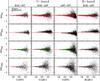 |
Fig. 2 Differences between magnitudes obtained using different cameras for common galaxies (black dots) as a function of magnitude. The plots in the topmost row of the figure refer to the total magnitudes, while those in the remaining rows refer to the magnitudes within circular apertures of radii 2, 5, and 10 kpc, top to bottom. The plots in the rightmost column of the figure refer to the B-band, while those in the other columns refer to the U-band. The red dots in the plots of the topmost row of the figure (total magnitudes) refer to the stars. The green curves in the plots relative to the 5 kpc apertures (third row of the figure) illustrate the rms expected according to the formulas reported in the headers of the catalogs (see text for details). |
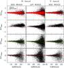 |
Fig. 3 Differences between optical bands (B,V) magnitudes from the catalogs presented here and the corresponding magnitudes in the original WINGS optical survey as a fuction of WINGS magnitudes for the galaxies in common (black dots). The plots in the topmost row of the figure refer to the total magnitudes, while those in the remaining rows refer to the magnitudes within circular apertures of radii 2, 5, and 10 kpc, top to bottom. The plots in the rightmost column of the figure refer to the V-band, while those in the other columns refer to the B-band. The red dots in the plots of the topmost row (total magnitudes) and the green curves in the plots relative to the 5 kpc apertures (third row) are the same as in Fig. 2. |
4. Data quality
4.1. Internal comparisons
In Fig. 2 we show the differences between magnitudes obtained using different cameras for common objects (black and red dots for galaxies and stars, respectively) as a function of magnitude of one of the two cameras, typically the one providing the most reliable values. The green curves in the plots relative to the 5 kpc apertures (third row of the figure) illustrate the rms expected according to the formulas reported in the headers of the catalogs (see last sentence of Sect. 3) as a function of magnitude. In particular, for each couple of cameras to be compared, the rms (green) curve was obtained using the error propagation rules to combine the rms formulas (reported in the catalog header) of the common clusters for both cameras and weighting each rms formula according to the number of galaxies in the respective catalog. A quick overview of the photometric agreement among the INT, BOK, and LBT cameras for galaxies in common clusters is given in Table 5. Here, for each magnitude (total, 2 kpc, 5 kpc, and 10 kpc) and for each pairwise comparison, we list the median value and the rms (in parenthesis) of the magnitude differences up to a given total apparent magnitude (19.5, in the B- and U-band).
Median values and rms (in parenthesis) of the magnitude differences for internal comparisons.
From Fig. 2 and Table 5, the agreement among the U-band magnitudes of the different cameras is generally good, although for the median values this comparison test is meaningful only for the INT magnitudes, since both the BOK and LBT magnitudes were calibrated on the SDSS magnitudes. The same holds for the BOK-LBT comparison of the B-band magnitudes (plots in the rightmost column of the figure). In fact, since the BOK and LBT B-band magnitudes have been both calibrated on the WINGS optical survey, again this comparison only provides a consistency test.
From Fig. 2, the only remarkable (and systematic) disagreement among the cameras concerns the magnitudes within circular apertures of radius 2 kpc. In this case the average differences reflect both the different average seeing conditions relative to the different cameras and the peculiar seeing of the mosaic image of each cluster. The influence of the seeing already disappears in the case of the circular apertures of radius 5 kpc, for which also the scatter in the plots agrees reasonably well with the expected rms (green curves) and better than for the 10 kpc aperture magnitudes.
4.2. External comparisons
Figure 3 is similar to Fig. 2, but illustrates the quality of B- and V-band photometry through a comparison between the magnitudes listed in the catalogs presented here and the corresponding magnitudes from the WINGS optical survey. It is worth recalling that since the BOK and LBT optical magnitudes were both calibrated on the WINGS optical survey, this comparison only provides an estimate of the photometric quality (scatter) of the BOK and LBT data as a function of the WINGS magnitudes.
For Fig. 3 one could repeat the same considerations of the previous subsection (Fig. 2) for both the systematic disagreement of the magnitudes within circular apertures of radius 2 kpc and the expected rms as a function of the magnitude (green curves in the 5 kpc aperture magnitudes plots).
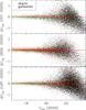 |
Fig. 4 Differences between U-band total magnitudes from the catalogs presented here and the corresponding magnitudes derived from the SDSS magnitudes using the the conversion formula by Lupton (2005) as a function of the SDSS magnitudes. Black and red dots in the plots refer to galaxies and stars, respectively. |
In Fig. 4 the U-band magnitudes of the present survey are compared with the corresponding U-band magnitudes derived from the SDSS database using the formula provided by Lupton (2005). Again, since the BOK and LBT U-band magnitudes were both calibrated on the SDSS data, the middle and bottom panels of the figure only provide an estimate of the photometric quality (scatter) of the BOK and LBT magnitudes as a function of SDSS data. Instead, the uppermost plot in the figure illustrates the fair agreement between the SDSS and INT U-band photometric zero-points. Table 6 is similar to Table 5, but refers to the external comparisons. In this case the limiting magnitudes adopted to compute the median values and the rms of the magnitude differences are 19.5 for the B- and U-band, while for the V-band we adopted Vlim = 20.5. Note that for the U-band comparisons we can only use the total magnitudes.
Median values and rms (in parenthesis) of the magnitude differences for external comparisons.
Although Table 6 and Figs. 3 and 4 refer to all clusters available for the different comparisons, we recorded the average magnitude differences for each individual cluster and for each magnitude (total and aperture magnitudes). These average differences are reported in the third group of rows of the header of each catalog (see Fig. 1). They may be useful to derive the catalog magnitudes (both total and aperture magnitudes) statistically consistent with the WINGS-OPT and SDSS magnitudes, thus allowing a more correct computation of galaxy colors (in particular, aperture colors) for each individual cluster. It is worth remarking, however, that significant differences between the catalog and comparison (WINGS-OPT and SDSS) magnitudes may persist, depending on the sizes and luminosity profiles of individual galaxies.
4.3. Photometric depth
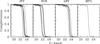 |
Fig. 5 Fractions of retrieved simulated galaxies as a function of the U-band total magnitudes for the four cameras. |
We used simulations to estimate the detection rate in the different bands as a function of the magnitude. In particular, for each field, we used the IRAF task mkobj with the true image PSF to produce a large number of artificial stars that were randomly distributed upon the field. In particular, the artificial galaxies were simulated by trying to reproduce the magnitude, size, and ellipticity distributions of the galaxies in the real image. Most artificial objects were simulated in the range of faint magnitudes, where SEx is less reliable. The artificial objects were added to the original frames and, on the new images, SEx was run using the same configuration files as for deriving the original catalogs. The resulting catalogs were matched with the catalogs of the artificial objects and the fraction of them recovered by SEx in each magnitude bin was recorded. Figure 5 illustrates the fractions of simulated galaxies retrieved by this procedure as a function of the U-band total magnitudes for the four cameras. Columns 4−6 of Table 4 list the range of 90% detection rates of artificial galaxies for each camera and filter. Moreover, the second group of rows in the headers of the catalogs (see Fig. 1) report the 90% detection rates of artificial galaxies for each band, cluster, and telescope. For simulated galaxies, the 90% detection rate in the U-band is reached at different magnitudes for different telescopes and clusters, spanning the intervals (22.30−23.30), (22.60–23.30) and (21.30–22.10) for the INT, LBT, and BOK imaging, respectively. The INT and LBT telescopes provided similar results, both in terms of photometric depth and stability. Instead, probably because of the poor weather conditions during the two observing runs, the photometric depth of the BOK images was poorer.
5. Conclusions
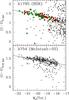 |
Fig. 6 Color–magnitude diagram (U − V) − MV for Abell 1795 (this work) and for Abell 754 (McIntosh et al. 2005). The straight lines in the plots correspond to the best-fit parameters given for Abell 754 in Table 8 of McIntosh et al. (2005) last row. The red and green dots in the upper panel, respectively mark elliptical and S0 galaxies that are spectroscopically confirmed members of the cluster Abell 1795. |
In Fig. 6 the (U − V) − MV color–magnitude diagram (CMD) of galaxies in Abell 1795 (upper panel, this work) is compared with the same diagram obtained for Abell 754 by McIntosh et al. (2005, lower panel in the figure). For Abell 1795, the colors refer to the 5 kpc apertures and the galaxies reported in the figure are those in common between the WINGS-OPT and BOK catalogs and morphologically classified by Fasano et al. (2012). The U- and V-band magnitudes are taken from the BOK and WINGS-OPT catalogs, respectively. The red and green dots in the plot represent the elliptical and S0 galaxies spectroscopically confirmed members of the cluster.
In spite of the uncertain data quality of the BOK imaging, the red sequence of the A1795 cluster members is very well defined. The two very blue S0 galaxies in the plot were visually inspected in the images. One of them is a close merger, the other one is very close to a bright star. Instead, the elliptical galaxy below the red sequence is undisturbed, but it is quite small (dwarf-like).
For Abell 754, the colors in the CMD refer to an aperture of 3.34 kpc and the straight line in the plot corresponds to the best-fit parameters given for this cluster in Table 8 of McIntosh et al. (2005, last row). The same straight line is also reported in the upper panel of Fig. 6. Although the CMDs are obtained with different apertures and for different clusters, the agreement of the two CMDs is quite satisfactory, thus making us confident about the good quality of our U-band photometry.
In a following paper of the series we will present and analyze the color–magnitude diagrams and the average color as a function of both the cluster-centric distance and the morphological type for all clusters belonging to the present sample and for the clusters included in our ongoing OmegaCam (VST) survey (six clusters already imaged in the U-band). Moreover, both sets of data will be used to validate the star formation rates and histories previously obtained for WINGS galaxies (Fritz et al. 2011) and to study the color map of individual galaxies at different distances and position angles with respect to the cluster center. This will help distinguishing between the various physical processes that are possibly responsible for the gas depletion in galaxies infalling into the clusters.
All the catalogues are available at the CDS.
Acknowledgments
We acknowledge partial financial support by contract PRIN/MIUR 2009: “Dynamics and Stellar Populations of Superdense Galaxies” (Code: 2009L2J4MN) and by INAF/PRIN 2011: “Galaxy Evolution with the VLT Survey Telescope (VST)”.
References
- Abazajian, K. N., Adelman-McCarthy, J. K., Agüeros, M. A., et al. 2009, ApJS, 182, 543 [NASA ADS] [CrossRef] [Google Scholar]
- Abell, G. O. 1958, ApJS, 3, 211 [NASA ADS] [CrossRef] [Google Scholar]
- Abraham, R. G., Smecker-Hane, T. A., Hutchings, J. B., et al. 1996, ApJ, 471, 694 [NASA ADS] [CrossRef] [Google Scholar]
- Balogh, M., Morris, S., Yee, H., Carlberg, R., & Ellingson, E. 1997, ApJ, 488, L75 [NASA ADS] [CrossRef] [Google Scholar]
- Barbaro, G., & Poggianti, B. M. 1997, A&A, 324, 490 [NASA ADS] [Google Scholar]
- Bertin, E. 2007, SCAMP v 1.3.5 Users guide [Google Scholar]
- Bertin, E., & Arnouts, S. 1996, A&AS, 117, 393 [NASA ADS] [CrossRef] [EDP Sciences] [Google Scholar]
- Blakeslee, J. P., Franx, M., Postman, M., et al. 2003, ApJ, 596, L143 [NASA ADS] [CrossRef] [Google Scholar]
- Cava, A., Bettoni, D., Poggianti, B. M., et al. 2009, A&A, 495, 707 [NASA ADS] [CrossRef] [EDP Sciences] [Google Scholar]
- Couch, W., Barger, A., Smail, I., Ellis, R., & Sharples, R. 1998, ApJ, 497, 188 [NASA ADS] [CrossRef] [Google Scholar]
- Couch, W. J., Balogh, M. L., Bower, R. G., et al. 2001, ApJ, 549, 820 [NASA ADS] [CrossRef] [Google Scholar]
- De Lucia, G., Poggianti, B. M., Aragón-Salamanca, A., et al. 2004, ApJ, 610, L77 [NASA ADS] [CrossRef] [Google Scholar]
- Desai, V., Dalcanton, J. J., Mayer, L., et al. 2004, MNRAS, 351, 265 [NASA ADS] [CrossRef] [Google Scholar]
- Dressler, A., Oemler, A. J., Couch, W., et al. 1997, ApJ, 490, 577 [NASA ADS] [CrossRef] [Google Scholar]
- Dresser, A., Smail, I., Poggianti, B., et al. 1999, ApJS, 122, 51 [NASA ADS] [CrossRef] [Google Scholar]
- Ebeling, H., Voges, W., Bohringer, H., et al. 1996, MNRAS, 281, 799 [NASA ADS] [CrossRef] [Google Scholar]
- Ebeling, H., Edge, A. C., Bohringer, H., et al. 1998, MNRAS, 301, 881 [NASA ADS] [CrossRef] [Google Scholar]
- Ebeling, H., Edge, A. C., Allen, S. W., et al. 2000, MNRAS, 318, 333 [NASA ADS] [CrossRef] [Google Scholar]
- Ellingson, E., Lin, H., Yee, H. K. C., & Carlberg, R. G. 2001, ApJ, 547, 609 [NASA ADS] [CrossRef] [Google Scholar]
- Fasano, G., Poggianti, B. M., Couch, W. J., et al. 2000, ApJ, 542, 673 [NASA ADS] [CrossRef] [Google Scholar]
- Fasano, G., Marmo, C., Varela, J., et al. 2006, A&A, 445, 805 [NASA ADS] [CrossRef] [EDP Sciences] [Google Scholar]
- Fasano, G., Vanzella, E., Dressler, A., et al. 2012, MNRAS, 420, 926 [NASA ADS] [CrossRef] [Google Scholar]
- Fritz, J., Poggianti, B. M., Cava, A., et al. 2011, A&A, 526, A45 [NASA ADS] [CrossRef] [EDP Sciences] [Google Scholar]
- Fukugita, M., Ichikawa, T., Gunn, J., et al. 1996, AJ, 111, 1748 [NASA ADS] [CrossRef] [Google Scholar]
- Galadi-Enriquez, D., Trullols, E., & Jordi, C. 2000, A&AS, 146, 169 [NASA ADS] [CrossRef] [EDP Sciences] [Google Scholar]
- Giallongo, E., Ragazzoni, R., Grazian, A., et al. 2008, A&A, 482, 349 [NASA ADS] [CrossRef] [EDP Sciences] [Google Scholar]
- Gladders, M. D., & Yee, H. K. C. 2005, ApJS, 157, 1 [NASA ADS] [CrossRef] [Google Scholar]
- Gomez, P. L., Nichol, R. C., Miller, C. J., et al. 2003, ApJ, 584, 210 [NASA ADS] [CrossRef] [Google Scholar]
- Grado, A., Capaccioli, M., Limatola, L., & Getman, F. 2010, MmSAIt, 15, 450 [Google Scholar]
- Jordi, K., Grebel, E. K., & Ammon, K. 2006, A&A, 460, 339 [NASA ADS] [CrossRef] [EDP Sciences] [Google Scholar]
- Halliday, C., Milvang-Jensen, B., Poirier, S., et al. 2004, A&A, 427, 397 [NASA ADS] [CrossRef] [EDP Sciences] [Google Scholar]
- Kennicutt, R. C. 1998, ApJ, 498, 541 [NASA ADS] [CrossRef] [Google Scholar]
- Kodama, T., & Bower, R. 2003, MNRAS, 346, 1 [NASA ADS] [CrossRef] [Google Scholar]
- Kodama, T., Smail, I., Nakata, F., et al. 2001, ApJ, 562, L9 [Google Scholar]
- Kodama, T., Balogh, M. L., Smail, I., et al. 2004, MNRAS, 354, 1103 [NASA ADS] [CrossRef] [Google Scholar]
- Landolt, A. U. 1992, AJ, 104, 372 [NASA ADS] [CrossRef] [Google Scholar]
- Lewis, I., Balogh, M., De Propris, R., et al. 2002, MNRAS, 334, 673 [NASA ADS] [CrossRef] [Google Scholar]
- Lupton, R. H. 2005, https://www.sdss3.org/dr8/algorithms/sdssUBVRITransform.php [Google Scholar]
- Marmo, C. 2003, Ph.D. Thesis, Padova [Google Scholar]
- McIntosh, D. H., Rix, H.-W., & Caldwell, N. 2004, ApJ, 610, 161 [Google Scholar]
- McIntosh, D. H., Zabludoff, A. I., Rix, H.-W., & Caldwell, N. 2005, ApJ, 619, 193 [NASA ADS] [CrossRef] [Google Scholar]
- Pignatelli, E., Fasano, G., & Cassata, P. 2006, A&A, 446, 373 [NASA ADS] [CrossRef] [EDP Sciences] [Google Scholar]
- Pimbblet, K. A., Smail, I., Kodama, T., et al. 2002, MNRAS, 331, 333 [NASA ADS] [CrossRef] [Google Scholar]
- Poggianti, B. M., Smail, I., Dressler, A., et al., 1999, AJ, 518, 576 [NASA ADS] [CrossRef] [Google Scholar]
- Poggianti, B. M., Bridges, T. J., Komiyama, Y., et al. 2004, ApJ, 601, 197 [NASA ADS] [CrossRef] [Google Scholar]
- Radovich, M., Arnaboldi, M., Ripepi, V., et al. 2004, A&A, 417, 51 [NASA ADS] [CrossRef] [EDP Sciences] [Google Scholar]
- Solanes, J. M., Manrique, A., García-Gómez, C., et al. 2001, ApJ, 548, 97 [NASA ADS] [CrossRef] [Google Scholar]
- Speziali, R., Di Paola, A., Giallongo, E., et al. 2008, SPIE, 7014, 70144T [CrossRef] [Google Scholar]
- Stetson, P. B. 1987a, PASP, 99, 191 [NASA ADS] [CrossRef] [Google Scholar]
- Stetson, P. B. 1987b, BAAS, 19, 745 [NASA ADS] [Google Scholar]
- Stetson, P. B. 1994, in Photometry with a Variable PSF, Proc. of the Workshop held in Quebec City, P.Q., Canada, 72 [Google Scholar]
- Stetson, P. B. 2000, PASP, 112, 925 [NASA ADS] [CrossRef] [Google Scholar]
- Stone, R. C. 1997, AJ, 114, 2811 [NASA ADS] [CrossRef] [Google Scholar]
- Treu, T., Ellis, R. S., Kneib, J.-P., et al. 2003, ApJ, 591, 53 [NASA ADS] [CrossRef] [Google Scholar]
- Valentinuzzi, T., Woods, D., Fasano, G., et al. 2009, A&A, 501, 851 [NASA ADS] [CrossRef] [EDP Sciences] [Google Scholar]
- Varela, J., D’Onofrio, M., Marmo, C., et al. 2009, A&A, 497, 667 [NASA ADS] [CrossRef] [EDP Sciences] [Google Scholar]
All Tables
Median values and rms (in parenthesis) of the magnitude differences for internal comparisons.
Median values and rms (in parenthesis) of the magnitude differences for external comparisons.
All Figures
|
Fig. 1 Header and first rows of the catalog from BOK imaging of A1795. |
| In the text | |
|
Fig. 2 Differences between magnitudes obtained using different cameras for common galaxies (black dots) as a function of magnitude. The plots in the topmost row of the figure refer to the total magnitudes, while those in the remaining rows refer to the magnitudes within circular apertures of radii 2, 5, and 10 kpc, top to bottom. The plots in the rightmost column of the figure refer to the B-band, while those in the other columns refer to the U-band. The red dots in the plots of the topmost row of the figure (total magnitudes) refer to the stars. The green curves in the plots relative to the 5 kpc apertures (third row of the figure) illustrate the rms expected according to the formulas reported in the headers of the catalogs (see text for details). |
| In the text | |
|
Fig. 3 Differences between optical bands (B,V) magnitudes from the catalogs presented here and the corresponding magnitudes in the original WINGS optical survey as a fuction of WINGS magnitudes for the galaxies in common (black dots). The plots in the topmost row of the figure refer to the total magnitudes, while those in the remaining rows refer to the magnitudes within circular apertures of radii 2, 5, and 10 kpc, top to bottom. The plots in the rightmost column of the figure refer to the V-band, while those in the other columns refer to the B-band. The red dots in the plots of the topmost row (total magnitudes) and the green curves in the plots relative to the 5 kpc apertures (third row) are the same as in Fig. 2. |
| In the text | |
|
Fig. 4 Differences between U-band total magnitudes from the catalogs presented here and the corresponding magnitudes derived from the SDSS magnitudes using the the conversion formula by Lupton (2005) as a function of the SDSS magnitudes. Black and red dots in the plots refer to galaxies and stars, respectively. |
| In the text | |
|
Fig. 5 Fractions of retrieved simulated galaxies as a function of the U-band total magnitudes for the four cameras. |
| In the text | |
|
Fig. 6 Color–magnitude diagram (U − V) − MV for Abell 1795 (this work) and for Abell 754 (McIntosh et al. 2005). The straight lines in the plots correspond to the best-fit parameters given for Abell 754 in Table 8 of McIntosh et al. (2005) last row. The red and green dots in the upper panel, respectively mark elliptical and S0 galaxies that are spectroscopically confirmed members of the cluster Abell 1795. |
| In the text | |
Current usage metrics show cumulative count of Article Views (full-text article views including HTML views, PDF and ePub downloads, according to the available data) and Abstracts Views on Vision4Press platform.
Data correspond to usage on the plateform after 2015. The current usage metrics is available 48-96 hours after online publication and is updated daily on week days.
Initial download of the metrics may take a while.