| Issue |
A&A
Volume 561, January 2014
|
|
|---|---|---|
| Article Number | A90 | |
| Number of page(s) | 5 | |
| Section | Cosmology (including clusters of galaxies) | |
| DOI | https://doi.org/10.1051/0004-6361/201322637 | |
| Published online | 08 January 2014 | |
Research Note
On the contribution of active galactic nuclei to reionization
Center for Relativistic Astrophysics, School of Physics, Georgia Institute of Technology, 837 State Street, Atlanta, GA 30332-0430, USA
e-mail: rgrissom6@gatech.edu
Received: 9 September 2013
Accepted: 27 November 2013
The electron scattering optical depth constraints on reionization suggest that there may be other sources that contribute to the ionization of hydrogen aside from observable star forming galaxies. Often the calculated value of the electron scattering optical depth, τes, falls below the measurements derived from observations of the cosmic microwave background, or an assumption about non-observable sources must be made in order to reach agreement. Here, we calculate the hydrogen ionization fraction as a function of redshift and the electron scattering optical depth from both galaxies and active galactic nuclei (AGN) factoring in the secondary collisional ionizations from the AGN X-ray emission. In this paper we use the most current determination of the evolving hard X-ray luminosity function and extrapolate its evolution beyond z = 6. The AGN spectral energy distributions include both UV and X-ray ionizing photons. To search for the largest possible effect, all AGNs are assumed to have λEdd = 1.0 and to be completely unobscured. The results show that AGNs produce a perturbative effect on the reionization of hydrogen and they remain in agreement with current constraints. Our calculations find the epoch of reionization still ends at z ≈ 6 and only increases the electron scattering optical depth by ~2.3% under ideal conditions. This can only be moderately increased by assuming a constant black hole mass of MBH = 105 M⊙. As a result, we conclude that there is a need for other sources beyond observable galaxies and AGNs that contribute to the reionization of hydrogen at z > 6.
Key words: galaxies: active / galaxies: evolution / dark ages, reionization, first stars / quasars: general
© ESO, 2014
1. Introduction
Most recent studies agree that star forming galaxies are the dominant contributors to the reionization of hydrogen in the universe (Alvarez et al. 2012; Haardt & Madau 2012; Robertson et al. 2013), with other sources, such as active galactic nuclei (AGN) and X-ray binaries, being sub-dominant to this process (Willott et al. 2010; Fontanot et al. 2012; McQuinn 2012; Holley-Bockelmann et al. 2012). While stars and detectable galaxies satisfy most constraints on the reionization of hydrogen, including ending at z ≈ 6, there is a consistent disagreement between the calculated and the observed electron scattering optical depth, τes, with the calculated values falling in the low region of the 68% range of the measured value. Alvarez et al. (2012) calculate a value of τes = 0.086 (in agreement with the seven-year WMAP best fit value; Komatsu et al. 2011) under the assumption of two galaxy types: low-mass galaxies with a high escape fraction (fesc = 0.8) and high-mass galaxies with low escape fraction (fesc = 0.05). The high-mass galaxies dominate reionization for z > 8, but are faint and below the current detection limit, while the low-mass galaxies dominate for z < 8 (Alvarez et al. 2012). When using a constant escape fraction fesc = 0.2 for the low-mass galaxies Alvarez et al. (2012) find only τes = 0.06. Similarly, Ahn et al. (2012) find τes = 0.0603, which is well below the seven-year WMAP measurements, but by including Pop. III stars as a source, they are able to increase τes to 0.0861. Robertson et al. (2013) determined the reionization history using star-forming galaxies to a limiting magnitude of MUV < −13 with an escape fraction of 0.2 and find τes ≈ 0.071, which is below the best fit value of 0.084 ± 0.013 for the electron scattering optical depth from the nine-year WMAP measurement (Hinshaw et al. 2012). Using a population of star-forming galaxies to a limiting magnitude of MUV < −17, which includes only detectable galaxies, yielded an even lower value for τes. They also considered a population down to a limiting magnitude of MUV < −10, which includes a number of undetectable galaxies. This resulted in a value of τes closer to the best-fit value, but also resulted in reionization ending closer to z ~ 7, further suggesting that there are other sources of reionization beyond low luminosity galaxies.
It is expected that including AGN as a source for reionization will have a perturbative effect rather than a significant one, but it should still increase the calculated electron scattering optical depth. In the Haardt & Madau (2012) model of reionization, they conclude that the UV emission from galaxies is the main contributor to reionization of hydrogen sufficient for meeting all existing constraints on this process, including τes. Willott et al. (2010) calculated that at z = 6 the quasar population contributes ≤20% of the photons required to maintain ionization. McQuinn (2012) concluded that faint quasars could not be solely responsible for the reionization of both hydrogen and helium and remain in agreement with constraints on both histories, specifically the redshifts at which each epoch ends. Alternatively, Volonteri & Gnedin (2009) modeled the growth and evolution of large and small massive black hole seeds over time and find that at z ≈ 6 quasars contribute ≤20% to the total number of ionizations, but at z ≈ 8 they could contribute from 50% to 90% of ionizations.
Here, we present a new, observationally-motivated calculation to investigate the optimal contribution of AGN as a means of reducing the variation in the calculated and measured values of τes. The most current parametization of the evolving hard X-ray AGN luminosity function (Hiroi et al. 2012) is used to compute the density of AGN ionizing photons. We also include the effects of secondary collisional ionizations from X-rays, as well as the UV emission from star forming galaxies. Since the focus of this calculation is to determine the maximum contribution to τes from AGN, we assume that all AGNs accrete at the same constant Eddington rate and are 100% unobscured. Variations in the Eddington ratio and the X-ray spectral slope are considered to determine the ideal contribution of AGN to the reionization of hydrogen. This simple calculation is independent of models of black hole growth and will provide a new constraint on the AGN contribution to τes. The cosmological parameters adopted throughout this paper are H0 = 67.77 km s-1 Mpc-1, Ωm = 0.304,ΩΛ = 0.691, and Ωb = 0.0483 (Planck Collaboration 2014a,b). We reproduce the results from Robertson et al. (2013) for these updated parameters as the baseline for a pure star-forming galaxy source of reionization.
2. Calculations
2.1. Overview
The evolution of the comoving ionized fraction of hydrogen, x(z), over time is described by  (1)where ⟨ nH ⟩, in cm-3, is the average comoving number density of hydrogen atoms; ṅ is the number density production rate of total ionizations; and ⟨ trec ⟩, in s, is the average recombination time. For case B recombinations
 ![\begin{equation} \langle t_{\rm rec}\rangle^{-1} = [C_{\rm HII}\alpha_{\rm B}(T)(1+Y_{\rm p}/4X_{\rm p})\langle n_{\rm H}\rangle(1+z)^3], \label{eq:trec} \end{equation}](/articles/aa/full_html/2014/01/aa22637-13/aa22637-13-eq33.png) (2)where CHII is the clumping factor quantifying the inhomogeneity in the intergalactic medium (IGM), αB(T) is the case B recombination coefficient, and XP and YP are the present hydrogen and helium abundances, respectively. Following Robertson et al. (2013), the IGM temperature is assumed to be 20 000 K, giving αB = 2.59 × 10 -13 cm3 s-1 and CHII = 3.0 (Pawlik et al. 2009).
(2)where CHII is the clumping factor quantifying the inhomogeneity in the intergalactic medium (IGM), αB(T) is the case B recombination coefficient, and XP and YP are the present hydrogen and helium abundances, respectively. Following Robertson et al. (2013), the IGM temperature is assumed to be 20 000 K, giving αB = 2.59 × 10 -13 cm3 s-1 and CHII = 3.0 (Pawlik et al. 2009).
The time-dependent production rate of ionizations, ṅ(z), depends on the source of ionizing photons. When considering an ionizing source of both star forming galaxies and AGN, the ionization production rate is ṅ = ṅGal + ṅAGN. For star forming galaxies, ṅGal can be estimated as  (3)where fesc is the escape fraction of ionizing photons, ξion is the hydrogen ionizing photons per 1500
  luminosity, and ρUV is the integrated luminosity density down to a limiting magnitude, MUV < −13 (we note that this includes objects below the current detection limits). From Robertson et al. (2013), fesc = 0.2 and ξion = 1025.2 Hz erg-1.
2.2. AGN Ionization production rate
The AGN contribution is defined  (4)with N(x,LX), in s-1, giving the total ionizations (including secondary collisional ionizations) occurring per second for a single AGN with rest-frame X-ray luminosity LX = L2−10 keV (in erg s-1) and surrounded by a medium in which the fraction of ionized hydrogen is x. The limits of the integration are log LX(min) = 41.5 and log LX(max) = 48. We adopt the X-ray luminosity function (dΦ/dlog LX) from the work of Hiroi et al. (2012) who determined the power-law decline at higher redshifts. We note that while this model is derived based on observable data to redshift z ≈ 4.5 (Hiroi et al. 2012) there are no data to confirm the accuracy of this luminosity function extrapolated to redshift z = 30. However, below we compare our ṅAGN at z = 6 with Willott et al. (2010) to justify this extrapolation.
To calculate the ionization rate produced by a single AGN,  (5)where LE(E) is the spectral energy distribution (SED) with units erg s-1 keV-1. Since the energy spectrum of an AGN includes a significant number of high-energy photons, the total number of ionizations per photon with initial energy, E, and background ionized hydrogen fraction, x, depends on the number of secondary collisional ionizations, χ(x,E). Shull & van Steenberg (1985) found that for a photon with initial energy E ≥ 100 eV in a medium with an ionized hydrogen fraction, x, the number of secondary collisional ionizations of hydrogen is best described as
  (6)with parameters C = 0.3908,a = 0.4092, and b = 1.7592 and an ionization energy EI = 13.6 eV. This analytic fit is only valid for an initial energy ≥100 eV. As the simulations also show that χ is a linear function of energy, E, for a fixed ionized fraction, x (Shull & van Steenberg 1985), we linearly extrapolate this relationship for energies E ≤ 100 eV.
To construct the SED for an AGN with a given X-ray luminosity LX, we start with the general shape: ![\begin{equation} L_E(E) = N \left[ \left(\frac{E}{h}\right)^{\alpha_{\rm UV}} \exp{(-E / k T_{\rm BB})} + a \left(\frac{E}{h}\right)^{1-\Gamma} \exp{(-E/E_{\rm cut})}\right].\label{eq:SED} \end{equation}](/articles/aa/full_html/2014/01/aa22637-13/aa22637-13-eq75.png) (7)The first term represents the thermal accretion disk spectrum, where αUV = −0.5 is the UV spectral slope and TBB is the characteristic blackbody temperature of the disk. The second term is the X-ray power-law spectrum, where Γ is the X-ray photon index and N is an overall normalization factor in order to give the needed LX. The exponential in the second term is a high-energy cut-off Ecut = 300 keV (e.g, Ricci et al. 2011).
(7)The first term represents the thermal accretion disk spectrum, where αUV = −0.5 is the UV spectral slope and TBB is the characteristic blackbody temperature of the disk. The second term is the X-ray power-law spectrum, where Γ is the X-ray photon index and N is an overall normalization factor in order to give the needed LX. The exponential in the second term is a high-energy cut-off Ecut = 300 keV (e.g, Ricci et al. 2011).
To connect the X-ray power law to the optical emission, we use the αox parameter,  (8)which defines the slope between the optical spectrum and the X-ray spectrum. As αox is a measure of the relative strength of the X-ray emission, it is observed to be correlated with κBol = LBol/LX, the X-ray bolometric correction (Lusso et al. 2010). In turn, κBol is related to λEdd = LBol/LEdd (Lusso et al. 2010), and LBol and LEdd are the bolometric luminosity and the Eddington luminosity, respectively. Thus, for a given LX and λEdd a corresponding κBol and αox are calculated. From the bolometric correction, the black hole mass is determined via LEdd = (1.38 × 1038)(MBH/M⊙)erg s-1. This yields the characteristic blackbody temperature, TBB = 1.37 × 10⁷(MBH/M⊙)− 1/4 K, needed to determine the optical bump in the SED. Figure 1 shows an example SED. As a check, this SED is integrated from 1μm to 1000 keV to calculate a bolometric luminosity of 1046.4 erg s-1m, which is only 2.5 times larger than the empirical luminosity, LBol = κBolLX = 1046 erg s-1. Given the uncertainties in measuring κBol and the true AGN SED, this result supports the methods used in this paper.
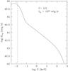 |
Fig. 1 General form of the spectral energy distribution for a single AGN given by Eq. (7) with an accretion rate of λEdd = 1.0. For this particular AGN, Γ = 2.5 and the UV to X-ray correlation parameter is αox = −1.73. The dashed line represents E = 13.6 eV. |
The SED in our calculation is defined entirely by three parameters: LX, Γ, and λEdd. Given values for these quantities, we can construct an SED for any AGN. It should be noted that for the entire population the ideal assumption is made that all AGN accrete at the same λEdd.
Once the SED is computed from Eq. (7), then ṅAGN can be calculated from Eqs. (5) and (6). As an example, Fig. 2 shows the ionizing photon production rate solely from AGN, ṅphoton, versus the AGN ionization production rate, ṅAGN, for an accretion rate of λEdd = 1.0 and Γ = 2.5. Although we consider various values of Γ for a fixed λEdd = 1.0, Brightman et al. (2013) determined that there is a strong correlation between Γ and λEdd; for λEdd = 1.0, Γ ≈ 2.3. As a result, we consider λEdd = 1.0 and Γ = 2.5 to be our ideal case. Since the number of total ionizations is directly dependent on the ionized fraction at any given redshift, z, the evolution of x attributable to the star forming galaxies listed in Robertson et al. (2013) is used to produce ṅAGN. Although this is not entirely self-consistent, it is known that AGN do not change the evolution of x(z) significantly, so it is sufficient to use the Robertson et al. (2013) results to demonstrate the effects of secondary collisional ionizations. As expected, at higher redshift when the ionization fraction drops, there appears to be more ionizations than photons as a result of collisional ionizations within a partially-ionized medium. By decreasing λEdd from 1.0 to 0.1 the ratio of ionizations to ionizing photons at z = 10 increases from ≈1.1 to ≈1.25. This increase in collisional ionizations results from the higher contribution of X-rays to the bolometric luminosity based on the definitions of λEdd and κbol. However, although there may be 15% more ionizations compared to the number of available ionizing photons for a lower Eddington ratio, the total number of ionizing photon decreases overall. Changing the photons index, on the other hand, has very little effect. The minimum ratio occurs for Γ = 2.0 and increases only slightly by either decreasing or increasing Γ.
For this highly idealized model of an AGN source, log ṅAGN ≈ 50.1 at z = 6 for the optimal scenario of Γ = 2.5 and λEdd = 1.0. Checking this against the work of Willott et al. (2010), in which they derived the luminosity function at redshift 6 using a sample of 40 quasars, our results show a slightly higher ionizing photon production rate than their maximum allowed value of log ṅAGN = 49.4; yet, our value for ṅAGN is still within a factor of 5 of their upper bound estimate. Given the simplifications made in our model, this is very reasonable.
Equations (4) and (1) are solved simultaneously using a fourth-order Runge-Kutta method to calculate the fraction of ionized hydrogen. At redshift z = 30, x is assumed to be 10-5 for the initial conditions. Although an escape fraction is assumed for the photon emissivity from the galaxies, no such constraint is made for the AGN. Assuming that 100% of ionizing photons escape from all AGN means that obscuration is not being taken into account and that the results given in the next section are idealized maximum cases.
2.3. Electron scattering optical depth
One of the main constraints on the reionization history is the electron scattering optical depth of the IGM. Using the ionization fraction, x(z), found by solving Eq. (1), the optical depth is computed as  (9)where c is the speed of light, σT is the Thompson cross section, and fe is the number of free electrons in the IGM per a hydrogen nucleus. The last quantity depends on the ionization of both helium and hydrogen. Alvarez et al. (2012) defined the break redshift at which helium goes from being singly ionized to doubly ionized at z = 3, and Robertson et al. (2013) define this point to be at z = 4. In keeping consistent with the work of Robertson et al. (2013), fe = (1 + Yp/2Xp) for z ≤ 4 and fe = (1 + Yp/4Xp) for z > 4.
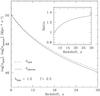 |
Fig. 2 Comparison of the production rate of ionizing photons and the rate of actual ionizations, including secondary collisional ionizations. This is the maximum ideal case where all AGN are assumed to accrete at a rate of λEdd = 1.0 and the X-ray photon index is Γ = 2.5. The difference between the two curves increases as redshift increases, where the IGM becomes more and more neutral. The hydrogen ionization fraction, x, used to calculate ṅAGN in Eq. (4) is due solely to the star-forming galaxies calculated by Robertson et al. (2013). Important to note that even though the high-energy photons cause additional ionizations, the number remains below ṅ ≈ 2 − 4 × 1050 Mpc-3 as seen in the work of Alvarez et al. (2012) for the galactic ionization production rate. The inset shows the ratio of ionizations to ionizing photons. |
3. Results
3.1. Contribution of AGN to the ionized hydrogen fraction
The left panel in Fig. 3 shows the ionization fraction found by solving Eq. (1) for three different sources of ionization: the Robertson et al. (2013) results for galaxies, galaxies and AGN with λEdd = 1.0 and Γ = 2.5, and galaxies and AGN with λEdd = 1.0 and Γ = 1.7. As expected from the previous works of Fontanot et al. (2012); Willott et al. (2010); and Haardt & Madau (2012), the addition of AGN appears to be a perturbation of the galactic contribution, with no dramatic change in the time at which reionization ends. Without an AGN contribution to reionization, hydrogen is completely ionized at z = 6. In the optimal case, λEdd = 1.0 and Γ = 2.5, reionization ends at z = 6.26. It ends at z = 6.13 for Γ = 1.7.
To better observe the effects of AGN on reionization, the percent difference (Δx/x = (xAGN − xGal)/xGal) is calculated and shown in the right panel of Fig. 3. A maximum 14% increase in the ionization fraction of hydrogen is observed near z ~ 6 for Γ = 2.5 and λEdd = 1.0 and only a maximum 8% increase is observed around the same time for Γ = 1.7. Decreasing the Eddington ratio to 0.1 reduces the effect of the AGN source from a ≈10% increase to a ≈1% increase (for varying values of Γ) in x near reionization.
3.2. Electron scattering optical depth
The effects of AGN on τes are shown in Fig. 4. For the star forming galaxies in Robertson et al. (2013), τes = 0.067 when calculated over 0 ≤ z ≤ 30. We note this is slightly lower than the value of τes ≈ 0.071 reported by Robertson et al. (2013). This is mainly due to the use of the Planck cosmological parameters instead of the nine-year WMAP parameters employed by Robertson et al. (2013). Including AGN with an accretion rate of λEdd = 1.0 increases τes to 0.0684 for Γ = 2.5 and to 0.0678 for Γ = 1.7. These results are equivalent to an overall ~2.3% increase and ~1.1% increase, respectively and represent the maximum contributions observed for our idealized model of AGN as an ionizing source. This further supports the observation that an AGN source of reionization acts as a perturbation of the dominant galactic contribution.
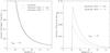 |
Fig. 3 Left panel: ionized hydrogen fraction x(z) for (1) a star-forming galaxy source (Robertson et al. 2013) (solid line); (2) galaxies plus AGN with λEdd = 1.0 and Γ = 2.5 (long-dashed line); and (3) galaxies plus AGN with λEdd = 1.0 and Γ = 1.7 (dotted line). All three cases show reionization ending around z ~ 6. Right panel: percent difference in the ionization fraction between each AGN case and the galaxy case as a function of redshift. In the ideal case, there is a maximum 14% increase in x near the end of reionization. |
Compared to the measurement of  (Planck Collaboration 2014b) derived from combining the Planck observations and WMAP polarization, all of the results shown in Fig. 4 fall below the best-fit value and lower end of this range. This suggests there may be other sources of reionization. Alvarez et al. (2012) studied the possibility of high-mass, low luminosity galaxies that fall below the current detection limit as a main contribution to reionization at high redshifts. Their work reproduces the measured WMAP and Planck constraint on τes. Robertson et al. (2013) also investigated the contribution of faint galaxies (below the current detectable limit) for three different limiting magnitudes, MUV: −10, −13, and −17. They find that considering only the detectable galaxies (MUV < −17) cannot reionize the Universe by z ≈ 6 and τes ≈ 0.05, falling well below the Planck results. Considering galaxies down to MUV = −10 yields τes ≈ 0.075, which lies just within the 68% margin of the Planck measurements, but reionization ends closer to z = 7. Using binary population synthesis simulations and observations from the present to z ≈ 4, Fragos et al. (2013) studied the evolution of X-ray binaries (XRBs) and their high energy contributions to the IGM. Their results suggest that while AGN are the dominant X-ray sources for 0 ≤ z ≤ 4, XRBs dominate the X-ray energy contribution to the IGM for 6 ≤ z ≤ 8 and most likely for higher redshifts as well. Thus, it is possible that these XRBs contribute more significantly to reionization than AGN. Simulating reionization with and without the very first stars formed in the Universe, Ahn et al. (2012) found that these stars contribute ~0.1−0.2 to the electron scattering optical depth. Including Pop. III brings their calculated value of τes to a value in agreement with Planck. The low values of τes calculated in this paper only for star forming galaxies with MUV ≤ −13 and AGN give support to these areas of study.
3.3. Constant MBH
We also briefly consider the scenario in which all AGN have the same constant black hole mass, MBH = 105 M⊙. Although this is not accurate at z = 6, for higher redshifts (z ≥ 8) this may be a more plausible scenario (Volonteri & Gnedin 2009). An AGN population with a constant black hole mass of 105 M⊙ has a higher accretion disk temperature and thus produces more ionizing photons than a population of AGN with just a constant λEdd.
Solving Eq. (1) assuming a constant black hole mass MBH = 105 M⊙ and an αox consistent with λEdd = 1.0, and Γ = 2.5 for all AGN, we find that reionization ends at z = 6.6, earlier than any of the results discussed in 3.1. This is evidence that a constant black hole mass is not viable around z ~ 6. Under these same conditions there is a 40% increase in the ionization fraction around z = 6, almost 3 times as great as the optimal increase mentioned in Sect. 3.1.
The contribution of AGN under this particular case also increases the electron scattering optical depth to τes = 0.071 corresponding to a 5.8% increase in τes when compared to just the contribution from star forming galaxies as in Robertson et al. (2013). Again, this increase is approximately 2.5 times greater than the optimal increase observed in Sect. 3.1, but still not significant enough to bring the calculated value of τes in agreement with the Planck measurements, providing evidence that further sources of reionization are needed. To finally settle the contribution of AGNs requires measures of quasar luminosity functions at z ≥ 6 by LSST, for example.
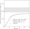 |
Fig. 4 Electron scattering optical depth for the same three cases as in Fig. 3: (1) a star-forming galaxy source (Robertson et al. 2013) (solid line); (2) galaxies plus AGN with λEdd = 1.0 and Γ = 2.5 (long-dashed line); and (3) galaxies plus AGN with λEdd = 1.0 and Γ = 1.7 (dotted line). Also shown is the evolution of τes for galaxies plus an AGN population with a constant black hole mass MBH = 105M⊙. The hatched region represents the most tightly constrained 68% margins of τes as measured by Planck Collaboration (2014b). All four cases fall below this region and, thus, below the best fit value of 0.089. |
4. Summary
We quantitatively evaluate the contribution of AGNs to reionization using the latest evolving hard X-ray AGN luminosity function, the consideration of secondary ionizations, and different values of λEdd and Γ. The effects of high-energy X-ray photons from the AGN are more perturbative than significant, in agreement with previous works (Willott et al. 2010; Fontanot et al. 2012; Haardt & Madau 2012; McQuinn 2012). Here, we consider an optimal, idealized model of AGN reionization, i.e. λEdd = 1.0 for all AGN, with no obscuration. Under these maximized conditions our results show that reionization still ends at z ≈ 6, but τes only increases by ≤2.3%, which is below the current Planck measurement. Despite looking at changes in Γ and λEdd, we find the only significant change in τes (an increase of ≈5.8%) follows from assuming a constant black hole mass of 105 M⊙ for the entire AGN population. However, this still yields a τes below the Planck value of  (Planck Collaboration 2014b). It may be possible for AGN to have a greater contribution to the reionization of hydrogen if the evolution of the AGN X-ray luminosity function dramatically alters at z ~ 10, but there is currently not enough observational data to support this type of evolution. Based on the small increase of τes, even with the best assumption of parameters to constrain this calculation, there is a need for additional perturbative sources to reionization at z > 6 other than AGN, such as X-ray binaries, Pop. III stars, and/or star forming galaxies that lie below current detection limits.
Acknowledgments
This work was supported in part by NSF awards AST 1008067 to D.R.B. and AST 1211626 to J.H.W.
References
- Ahn, K., Iliev, I. T., Shapiro, R., et al. 2012, ApJ, 756, L16 [NASA ADS] [CrossRef] [Google Scholar]
- Alvarez, M. A., Finlator, K., & Trenti, M. 2012, ApJ, 759, L38 [NASA ADS] [CrossRef] [Google Scholar]
- Brightman, M., Silverman, J. D., Mainieri, V., et al. 2013, MNRAS, 433, 2485 [NASA ADS] [CrossRef] [Google Scholar]
- Dunkley, J., Komatsu, E., Nolta, M. R., et al. 2009, ApJS, 180, 306 [NASA ADS] [CrossRef] [Google Scholar]
- Fontanot, F., Cristiani, S., & Vanzella, E. 2012, MNRAS, 425, 1413 [NASA ADS] [CrossRef] [Google Scholar]
- Fragros, T., Lehmer, B. D., Naoz, S., et al. 2013, ApJ, 776, L31 [NASA ADS] [CrossRef] [Google Scholar]
- Haardt, F., & Madau, P. 2012, ApJ, 746, 125 [NASA ADS] [CrossRef] [Google Scholar]
- Hinshaw, G., Larson, D., Komatsu, E., et al. 2012, ApJS, 208, 19 [Google Scholar]
- Hiroi, K., Ueda, Y., Akiyama, M., & Watson, M. 2012, ApJ, 758, 49 [NASA ADS] [CrossRef] [Google Scholar]
- Holley-Bockelmann, K., Wise, J. H., & Sinha, M. 2012, ApJ, 761, L8 [NASA ADS] [CrossRef] [Google Scholar]
- Komatsu, E., Smith, K., Dunkley, J., et al. 2011, ApJS, 192, 18 [NASA ADS] [CrossRef] [Google Scholar]
- Lusso, E., Comastri, A., Vignali, C., et al. 2010, A&A, 512, A34 [NASA ADS] [CrossRef] [EDP Sciences] [Google Scholar]
- McQuinn, M. 2012, MNRAS, 426, 1349 [NASA ADS] [CrossRef] [Google Scholar]
- Pawlik, A. H., Schaye, J., & van Scherpenzeel, E. 2009, MNRAS, 394, 1812 [NASA ADS] [CrossRef] [Google Scholar]
- Planck Collaboration 2014a, A&A, in press [arXiv:1303.5062] [Google Scholar]
- Planck Collaboration 2014b, A&A, in press [arXiv:1303.5076] [Google Scholar]
- Ricci, C., Walter, R., Courvoisier, T., et al. 2011, A&A, 532, A102 [NASA ADS] [CrossRef] [EDP Sciences] [Google Scholar]
- Robertson, B. E., Furlanetto, S. R., Schneider, E., et al. 2013, ApJ, 768, 71 [NASA ADS] [CrossRef] [Google Scholar]
- Shull, J. M., & van Steenberg, M. E. 1985, ApJ, 298, 268 [NASA ADS] [CrossRef] [Google Scholar]
- Volonteri, M., & Gnedin, N. Y. 2009, ApJ, 703, 2113 [NASA ADS] [CrossRef] [Google Scholar]
- Willott, C. J., Delorme, P., Reylé, C., et al. 2010, AJ, 139, 906 [NASA ADS] [CrossRef] [Google Scholar]
All Figures
|
Fig. 1 General form of the spectral energy distribution for a single AGN given by Eq. (7) with an accretion rate of λEdd = 1.0. For this particular AGN, Γ = 2.5 and the UV to X-ray correlation parameter is αox = −1.73. The dashed line represents E = 13.6 eV. |
| In the text | |
|
Fig. 2 Comparison of the production rate of ionizing photons and the rate of actual ionizations, including secondary collisional ionizations. This is the maximum ideal case where all AGN are assumed to accrete at a rate of λEdd = 1.0 and the X-ray photon index is Γ = 2.5. The difference between the two curves increases as redshift increases, where the IGM becomes more and more neutral. The hydrogen ionization fraction, x, used to calculate ṅAGN in Eq. (4) is due solely to the star-forming galaxies calculated by Robertson et al. (2013). Important to note that even though the high-energy photons cause additional ionizations, the number remains below ṅ ≈ 2 − 4 × 1050 Mpc-3 as seen in the work of Alvarez et al. (2012) for the galactic ionization production rate. The inset shows the ratio of ionizations to ionizing photons. |
| In the text | |
|
Fig. 3 Left panel: ionized hydrogen fraction x(z) for (1) a star-forming galaxy source (Robertson et al. 2013) (solid line); (2) galaxies plus AGN with λEdd = 1.0 and Γ = 2.5 (long-dashed line); and (3) galaxies plus AGN with λEdd = 1.0 and Γ = 1.7 (dotted line). All three cases show reionization ending around z ~ 6. Right panel: percent difference in the ionization fraction between each AGN case and the galaxy case as a function of redshift. In the ideal case, there is a maximum 14% increase in x near the end of reionization. |
| In the text | |
|
Fig. 4 Electron scattering optical depth for the same three cases as in Fig. 3: (1) a star-forming galaxy source (Robertson et al. 2013) (solid line); (2) galaxies plus AGN with λEdd = 1.0 and Γ = 2.5 (long-dashed line); and (3) galaxies plus AGN with λEdd = 1.0 and Γ = 1.7 (dotted line). Also shown is the evolution of τes for galaxies plus an AGN population with a constant black hole mass MBH = 105M⊙. The hatched region represents the most tightly constrained 68% margins of τes as measured by Planck Collaboration (2014b). All four cases fall below this region and, thus, below the best fit value of 0.089. |
| In the text | |
Current usage metrics show cumulative count of Article Views (full-text article views including HTML views, PDF and ePub downloads, according to the available data) and Abstracts Views on Vision4Press platform.
Data correspond to usage on the plateform after 2015. The current usage metrics is available 48-96 hours after online publication and is updated daily on week days.
Initial download of the metrics may take a while.