| Issue |
A&A
Volume 561, January 2014
|
|
|---|---|---|
| Article Number | A34 | |
| Number of page(s) | 4 | |
| Section | The Sun | |
| DOI | https://doi.org/10.1051/0004-6361/201322547 | |
| Published online | 20 December 2013 | |
Research Note
Frequency variations of solar radio zebras and their power-law spectra
Astronomical Institute of the Academy of Sciences of the Czech Republic, 25165 Ondřejov, Czech Republic
e-mail: This email address is being protected from spambots. You need JavaScript enabled to view it.
Received: 27 August 2013
Accepted: 21 November 2013
Abstract
Context. During solar flares several types of radio bursts are observed. The fine striped structures of the type IV solar radio bursts are called zebras. Analyzing them provides important information about the plasma parameters of their radio sources. We present a new analysis of zebras.
Aims. Power spectra of the frequency variations of zebras are computed to estimate the spectra of the plasma density variations in radio zebra sources.
Methods. Frequency variations of zebra lines and the high-frequency boundary of the whole radio burst were determined with and without the frequency fitting. The computed time dependencies of these variations were analyzed with the Fourier method.
Results. First, we computed the variation spectrum of the high-frequency boundary of the whole radio burst, which is composed of several zebra patterns. This power spectrum has a power-law form with a power-law index –1.65. Then, we selected three well-defined zebra-lines in three different zebra patterns and computed the spectra of their frequency variations. The power-law indices in these cases are found to be in the interval between –1.61 and –1.75. Finally, assuming that the zebra-line frequency is generated on the upper-hybrid frequency and that the plasma frequency ωpe is much higher than the electron-cyclotron frequency ωce, the Fourier power spectra are interpreted to be those of the electron plasma density in zebra radio sources.
Key words: Sun: radio radiation / plasmas / turbulence
© ESO, 2013
1. Introduction
Zebra patterns (or zebras) are particularly fine structures that are observed in some type IV radio events in a very broad frequency band (see for example, Slottje 1972, 1981; Aurass & Chernov 1983; Jiřička et al. 2001; Aurass et al. 2003; Chernov et al. 2003; Chen et al. 2011, and others). The zebras are believed to be an important source of information on plasma parameters and processes in solar flares, but that depends on the model used.
To explain zebras, many mechanisms have been proposed (Kuijpers 1975; Zheleznayakov & Zlotnik 1975; Chernov 1976; Mollwo 1983; Winglee & Dulk 1986; Ledenev et al. 2001; Yasnov & Karlický 2004; Bárta & Karlický 2006; LaBelle et al. 2003; Kuznetsov & Tsap 2007; Zlotnik 2013); for a review of these models, see Chernov (2010).
The most frequently used model assumes that the zebra line emission occurs at the double plasma resonance  (1)where ωUH, ωpe, and ωce are the upper-hybrid, electron-plasma, and electron-cyclotron frequencies, and s is an integer harmonic number (e.g. Zlotnik 2013). However, there are also models based on interferometric effects (Bárta & Karlický 2006; Ledenev et al. 2006), trapping of the upper-hybrid waves in density resonators (LaBelle et al. 2003), and the ion-cyclotron maser (Treumann et al. 2011). Recently, Karlický (2013) proposed a model that considers the emission at the double upper-hybrid frequency, but the zebra lines are formed by a modulation of the emission by the magnetohydrodynamic wave.
Zebras are characterized not only by zebra lines, but also by the frequency variations of these zebra lines, especially in long-duration zebras, see for example, Chernov et al. (1998), Ning et al. (2000), and Chen et al. (2011). Similar frequency variations were found also for the lace bursts, which were given this name because of their lace-like form in the radio spectrum. The lace bursts are characterized by distinct high-frequency boundaries and their rapid frequency variations; see Karlický et al. (2001), where the power spectra of these variations were computed.
In the present paper, we used the same idea as for the lace bursts and compute the power spectra of the zebra frequency variation. Then we interpret these spectra as the spectra of plasma density variations in zebra radio sources.
The paper is organized as follows: in Sect. 2 we describe the data and analyze them. Section 3 summarizes the results. Finally, in Sect. 4 we discuss our results.
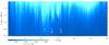 |
Fig. 1 Radio burst observed on August 1, 2010 at 08:16:40–08:26:40 UT by the Ondřejov radiospectrograph. The short white horizontal bars 1, 2, and 3 show intervals of the selected zebras presented in Figs. 2, 3, and 4, respectively. |
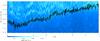 |
Fig. 2 Zebra pattern observed on August 1, 2010 at 08:20:16–08:20:23 UT by the Ondřejov radiospectrograph. This is the enlarged spectrum in the time interval corresponding to short white horizontal bar 1 in Fig. 1. The full line shows the computed frequency variations. |
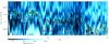 |
Fig. 3 Zebra pattern observed on August 1, 2010 at 08:21:01–08:21:06 UT by the Ondřejov radiospectrograph. This is the enlarged spectrum in the time interval corresponding to short white horizontal bar 2 in Fig. 1. The full line shows the computed frequency variations. |
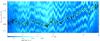 |
Fig. 4 Zebra pattern observed on August 1, 2010 at 08:21:55–08:22:01 UT by the Ondřejov radiospectrograph. This is the enlarged spectrum in the time interval corresponding to short white horizontal bar 3 in Fig. 1. The full line shows the computed frequency variations. |
2. Data and analysis
On 1 August 2010, during the GOES C3.2 flare (start 07:55 UT, maximum 08:26 UT, and end 09:35 UT), at 08:16:40–08:26:40 UT the Ondřejov radiospectrograph (Jiřička & Karlický 2008) recorded the radio spectrum shown in Fig. 1. The time and frequency resolution is 0.01 s and 4.7 MHz, respectively. The radio burst presented in this figure consists of several intervals with zebras. We selected the three longest and most distinct recorded zebras (see the three short white lines in Fig. 1 and the enlarged radio spectra in Figs. 2–4).
First, we determined a time dependance of the frequency variation of the high-frequency boundary of the whole burst. We selected some threshold in the radio emission flux that cuts the burst at some level. This cutting line gives us the high-frequency boundary of the burst. The threshold was selected in such a way that the resulting high-frequency boundary limits the selected zebras from the high-frequency sides. No frequency fitting was used in this long-duration burst (10 min), that is, the frequency resolution is the same as in the radio spectrum. The computed high-frequency boundary of the whole burst is shown in the upper part of Fig. 5.
Then we selected one very long zebra line in each of the selected zebras (Figs. 2–4) and computed its frequency variation in dependence on time. In these short-lasting cases (several seconds) we used a fitting procedure to increase the frequency resolution. We used the program that in each time step shows the frequency spectrum profile and positions of all maxima at this frequency profile through out the whole radio spectrum. This enabled us to find the frequency channel whose radio flux maximum corresponds to the selected zebra-line and also the radio fluxes in nearby channels. These radio flux values were then fitted by a Gaussian function, and we determined the central frequency of this Gaussian function. This gave us frequency variations of the selected zebra-line with an enhanced frequency resolution. The computed frequency variations are superimposed on the zebra radio spectra, see the full line in Figs. 2–4.
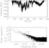 |
Fig. 5 Upper panel: frequency variations of the high-frequency boundary of the whole burst shown in Fig. 1. Bottom panel: power spectrum of these variations. |
3. Results
First, we computed the Fourier power spectrum of the frequency variations of the high-frequency boundary of the whole burst. The Fourier spectrum has a power-law form with a power-law index of about –1.65 (Fig. 5). Then we computed the Fourier spectra of the frequency variations of the selected three zebra lines. The results are shown in Figs. 6–8 as full lines. It is interesting that the power-law indices of the Fourier spectra of these zebra lines occur in the interval between –1.61 and –1.75, that is, close to −1.65 determined for the whole burst (Fig. 5).
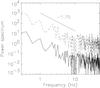 |
Fig. 6 Full line: power spectrum of the zebra-line frequency variations shown in Fig. 2. Dashed line: power spectrum of the computed plasma density variations (shifted in power for comparison with the frequency variations). The straight full line expresses the power-law index. |
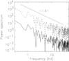 |
Fig. 7 Full line: power spectrum of the zebra-line frequency variations shown in Fig. 3. Dashed line: power spectrum of the computed plasma density variations (shifted in power for comparison with the frequency variations). The straight full line expresses the power-law index. |
4. Discussion and conclusions
We presented the Fourier spectra of frequency variations in solar radio zebras. These spectra were found to have a power-law form with power-law indices in the interval from –1.61 to –1.75. We found that the power-law index of the frequency variations in the whole burst with zebras is similar to those determined in selected zebra lines. This indicates that the same physical process causes the frequency variations in the whole burst and in zebras.
The Fourier spectra are power-law spectra, but at high frequencies the spectra are flat (in Fig. 5 above 3 Hz, in Figs. 6 and 8 above 10 Hz, and in Fig. 7 above 30 Hz). This is probably caused by a different noise level in the computed curves of the frequency variations. This agrees with the finding that the zebra lines shown in Fig. 3 are more distinct than those in Figs. 2 and 4.
The computed power-law indices are lower than those computed for the lace bursts (–1.88 to –2.13) in Karlický et al. (2001).
We assumed in the standard model that zebras are generated in the upper-hybrid frequency ωUH and that the plasma frequency ωpe is much higher than the electron-cyclotron frequency ωce in solar-flare conditions. Thus, relation (1) gives ωUH ≈ ωpe. Then, using the relation  , the frequency variations can be recalculated to those of the electron plasma density ne. We analyzed these recalculated data with the same Fourier method and show their power spectra with dashed lines in Figs. 6–8. As seen here, the power-law indices are the same as those for the frequency variations. The power-law indices in plasma density variations are close to the Kolmogorov turbulence spectral index (–1.66). This indicates that the plasma in the zebra radio sources is in turbulent state.
Our method shows a way to determine the power spectra of the electron plasma density in zebra radio sources. The disadvantage of this method is that the zebra lines are typically short and sometimes interrupted. On the other hand, we showed that a similar power-law index was found also for the whole burst with zebras, therefore in principle some bursts with zebras and a variable high-frequency boundary of the burst emission (like the burst shown in Fig. 1) could be used for this purpose.
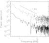 |
Fig. 8 Full line: power spectrum of the zebra-line frequency variations shown in Fig. 4. Dashed line: power spectrum of the computed plasma density variations (shifted in power for comparison with the frequency variations). The straight full line expresses the power-law index. |
Measurements of the density variations are basic in-situ procedures in any space mission. Thus, our results can be compared with those measured by spacecraft, for instance, in the solar wind (Šafránková et al. 2013). The density spectra in solar wind are also power-law spectra with a power-law index of about –1.48 in the low-frequency range (below about 0.5 Hz). At higher frequencies the spectrum is much steeper. The power-law index is –3.44. In comparison, our solar density spectra are power-law spectra until about 10 Hz. In these solar spectra there is no change of the spectral index similar to that in the solar-wind spectrum. However, many more examples of the solar density spectra are needed.
Acknowledgments
This research was supported by grants P209/12/0103 (GA CR), and the Marie Curie PIRSES-GA-2011-295272 RadioSun project. The author thanks Hana Mészárosová for the data preparation.
References
- Aurass, H., & Chernov, G. P. 1983, Sol. Phys., 84, 339 [NASA ADS] [CrossRef] [Google Scholar]
- Aurass, H., Klein, K.-L., Zlotnik, E. Y., & Zaitsev, V. V. 2003, A&A, 410, 1001 [NASA ADS] [CrossRef] [EDP Sciences] [Google Scholar]
- Bárta, M., & Karlický, M. 2006, A&A, 450, 359 [NASA ADS] [CrossRef] [EDP Sciences] [Google Scholar]
- Chen, B., Bastian, T. S., Gary, D. E., & Jing, J., 2011, ApJ, 736, 64 [NASA ADS] [CrossRef] [Google Scholar]
- Chernov, G. P. 1976, Sov. Astron., 20, 449 [Google Scholar]
- Chernov, G. P. 2010, Res. Astron. Astrophys., 10, 821 [NASA ADS] [CrossRef] [Google Scholar]
- Chernov, G. P., Markeev, A. K., Poquerusse, M., et al. 1998, A&A, 334, 314 [NASA ADS] [Google Scholar]
- Chernov, G. P., Yan, Y. H., & Fu, Q. J. 2003, A&A, 406, 1071 [NASA ADS] [CrossRef] [EDP Sciences] [Google Scholar]
- Jiřička, K., & Karlický, M. 2008, Sol. Phys., 253, 95 [NASA ADS] [CrossRef] [Google Scholar]
- Jiřička, K., Karlický, M., Mészárosová, H., & Snížek, V. 2001, A&A, 375, 243 [NASA ADS] [CrossRef] [EDP Sciences] [Google Scholar]
- Karlický, M. 2013, A&A, 552, A90 [NASA ADS] [CrossRef] [EDP Sciences] [Google Scholar]
- Karlický, M., Bárta, M., Jiřička, K., et al. 2001, A&A, 375, 638 [NASA ADS] [CrossRef] [EDP Sciences] [Google Scholar]
- Kuijpers, J. 1975, Sol. Phys., 44, 143 [Google Scholar]
- Kuznetsov, A. A., & Tsap, Yu. T. 2007, Sol. Phys., 241, 127 [NASA ADS] [CrossRef] [Google Scholar]
- LaBelle, J., Treumann, R. A., Yoon, P. H., & Karlický, M. 2003, ApJ, 593, 1195 [NASA ADS] [CrossRef] [Google Scholar]
- Ledenev, V. G., Karlický, M., Yan, Y., & Fu, Q. 2001, Sol. Phys., 202, 71 [NASA ADS] [CrossRef] [Google Scholar]
- Ledenev, V. G., Yan, Y., & Fu, Q. 2006, Sol. Phys., 233, 129 [NASA ADS] [CrossRef] [Google Scholar]
- Mollwo, L. 1983, Sol. Phys., 83, 305 [NASA ADS] [CrossRef] [Google Scholar]
- Ning, Z., Fu, Q., & Lu, Q. 2000, PASJ, 52, 919 [NASA ADS] [Google Scholar]
- Šafránková, J., Němeček, Z., Přech, L., et al. 2013, Space Sci. Rev., 175, 165 [NASA ADS] [CrossRef] [Google Scholar]
- Slottje, C. 1972, Sol. Phys., 25, 210 [NASA ADS] [CrossRef] [Google Scholar]
- Slottje, C. 1981, Atlas of fine structures of dynamic spectra of solar type IV-dm and some type II radio bursts (Dwingeloo: Netherlands Foundation for Radio Astronomy) [Google Scholar]
- Treumann, R. A., Nakamura, R., & Baumjohann, W. 2011, Ann. Geophys., 29, 1673 [NASA ADS] [CrossRef] [Google Scholar]
- Winglee, R. M., & Dulk, G. A. 1986, ApJ, 307, 808 [NASA ADS] [CrossRef] [Google Scholar]
- Yasnov, L. V., & Karlický, M. 2004, Sol. Phys., 219, 289 [NASA ADS] [CrossRef] [Google Scholar]
- Zheleznyakov, V. V., & Zlotnik, E. Y. 1975, Sol. Phys., 44, 461 [NASA ADS] [CrossRef] [Google Scholar]
- Zlotnik, E. Y. 2013, Sol. Phys., 284, 579 [NASA ADS] [CrossRef] [Google Scholar]
All Figures
|
Fig. 1 Radio burst observed on August 1, 2010 at 08:16:40–08:26:40 UT by the Ondřejov radiospectrograph. The short white horizontal bars 1, 2, and 3 show intervals of the selected zebras presented in Figs. 2, 3, and 4, respectively. |
| In the text | |
|
Fig. 2 Zebra pattern observed on August 1, 2010 at 08:20:16–08:20:23 UT by the Ondřejov radiospectrograph. This is the enlarged spectrum in the time interval corresponding to short white horizontal bar 1 in Fig. 1. The full line shows the computed frequency variations. |
| In the text | |
|
Fig. 3 Zebra pattern observed on August 1, 2010 at 08:21:01–08:21:06 UT by the Ondřejov radiospectrograph. This is the enlarged spectrum in the time interval corresponding to short white horizontal bar 2 in Fig. 1. The full line shows the computed frequency variations. |
| In the text | |
|
Fig. 4 Zebra pattern observed on August 1, 2010 at 08:21:55–08:22:01 UT by the Ondřejov radiospectrograph. This is the enlarged spectrum in the time interval corresponding to short white horizontal bar 3 in Fig. 1. The full line shows the computed frequency variations. |
| In the text | |
|
Fig. 5 Upper panel: frequency variations of the high-frequency boundary of the whole burst shown in Fig. 1. Bottom panel: power spectrum of these variations. |
| In the text | |
|
Fig. 6 Full line: power spectrum of the zebra-line frequency variations shown in Fig. 2. Dashed line: power spectrum of the computed plasma density variations (shifted in power for comparison with the frequency variations). The straight full line expresses the power-law index. |
| In the text | |
|
Fig. 7 Full line: power spectrum of the zebra-line frequency variations shown in Fig. 3. Dashed line: power spectrum of the computed plasma density variations (shifted in power for comparison with the frequency variations). The straight full line expresses the power-law index. |
| In the text | |
|
Fig. 8 Full line: power spectrum of the zebra-line frequency variations shown in Fig. 4. Dashed line: power spectrum of the computed plasma density variations (shifted in power for comparison with the frequency variations). The straight full line expresses the power-law index. |
| In the text | |
Current usage metrics show cumulative count of Article Views (full-text article views including HTML views, PDF and ePub downloads, according to the available data) and Abstracts Views on Vision4Press platform.
Data correspond to usage on the plateform after 2015. The current usage metrics is available 48-96 hours after online publication and is updated daily on week days.
Initial download of the metrics may take a while.