| Issue |
A&A
Volume 561, January 2014
|
|
|---|---|---|
| Article Number | A80 | |
| Number of page(s) | 9 | |
| Section | Cosmology (including clusters of galaxies) | |
| DOI | https://doi.org/10.1051/0004-6361/201322285 | |
| Published online | 03 January 2014 | |
Angular correlation of the cosmic microwave background in the Rh = ct Universe
Department of Physics, The Applied Math Program, and Department of
AstronomyThe University of Arizona,
Tucson,
Arizona,
85721
USA
e-mail:
This email address is being protected from spambots. You need JavaScript enabled to view it.
Received:
15
July
2013
Accepted:
5
December
2013
Abstract
Context. The emergence of several unexpected large-scale features in the cosmic microwave background (CMB) has pointed to possible new physics driving the origin of density fluctuations in the early Universe and their evolution into the large-scale structure we see today.
Aims. In this paper, we focus our attention on the possible absence of angular correlation in the CMB anisotropies at angles larger than ~60°, and consider whether this feature may be the signature of fluctuations expected in the Rh = ct Universe.
Methods. We calculate the CMB angular correlation function for a fluctuation spectrum expected from growth in a Universe whose dynamics is constrained by the equation-of-state p = −ρ/3, where p and ρ are the total pressure and density, respectively.
Results. We find that, though the disparity between the predictions of ΛCDM and the WMAP sky may be due to cosmic variance, it may also be due to an absence of inflation. The classic horizon problem does not exist in the Rh = ct Universe, so a period of exponential growth was not necessary in this cosmology in order to account for the general uniformity of the CMB (save for the aforementioned tiny fluctuations of 1 part in 100 000 in the WMAP relic signal).
Conclusions. We show that the Rh = ct Universe without inflation can account for the apparent absence in CMB angular correlation at angles θ ≳ 60° without invoking cosmic variance, providing additional motivation for pursuing this cosmology as a viable description of nature.
Key words: cosmic background radiation / cosmological parameters / cosmology: observations / cosmology: theory / dark matter / gravitation
John Woodruff Simpson Fellow.
© ESO, 2014
1. Introduction
The high signal-to-noise maps of the cosmic microwave background (CMB) anisotropies, particularly those produced by the Wilkinson Microwave Anisotropy Probe (WMAP; Bennett et al. 2003; Spergel et al. 2003) and, more recently, by Planck (Planck Collaboration 2013), have revolutionized our ability to probe the Universe on its largest scales. In the near future, even higher resolution temperature maps and high-resolution polarization maps, perhaps also tomographic 21-cm observations, will extend our knowledge of the Universe’s spacetime and its fluctuations to a deeper level, possibly probing beyond the surface of last scattering.
Yet the emergence of greater detail in these all-sky maps has revealed several possible unexpected features on large scales, some of which were first reported by the Cosmic Background Explorer (COBE) Differential Microwave Radiometer (DMR) collaboration (Wright et al. 1996). These include an apparent alignment of the largest modes of CMB anisotropy, as well as unusually low angular correlations on the largest scales.
Though viewed as significant anomalies at first (Spergel et al. 2003), these unexpected features may now be explained as possibly being due to cosmic variance within the standard model (Bennett et al. 2013). However, they may also be interesting and important for several reasons. Chief among them is the widely held view that the large-scale structure in the present Universe developed via the process of gravitational instability from tiny primordial fluctuations in energy density. The temperature fluctuations in the CMB, emerging several hundred thousand years after the big bang, are thought to be associated with the high-redshift precursors of the fluctuations that generated the galaxies and clusters we see today. Therefore, an absence of correlations in the CMB anisotropies may hint at required modifications to the standard model (ΛCDM), or possibly even new physics, each of which may alter our view of how the Universe came into existence and how it evolved from its earliest moments to the present state.
Our focus in this paper will be the possible absence of angular correlation in the CMB at angles larger than ~60°. This feature may be anomalous because the absence of any angular correlation at the largest scales would be at odds with the inflationary paradigm (Guth 1981; Linde 1982). But without inflation, ΛCDM simply could not account for the apparent uniformity of the CMB (other than fluctuations at the level of 1 part in 100 000 seen in the WMAP relic signal) across the sky. Thus, if variance is not the cause of the apparent disparity, the standard model of cosmology would be caught between contradictory observational constraints.
In this paper, we will therefore explore the possibility that these possible CMB anomalies might be understood within the context of the recently introduced Rh = ct Universe. This cosmology is motivated by a strict adherence to the requirements of the Cosmological Principle and the Weyl postulate, which together suggest that the Universe must be expanding at a constant rate. Additional theoretical support for this conclusion was reached with the recent demonstration that the Friedmann-Robertson-Walker (FRW) metric is apparently only valid for a perfect fluid with zero active mass, i.e., with ρ + 3p = 0, in terms of the total energy density ρ and pressure p (Melia 2013b); this is the equation-of-state that gives rise to the Rh = ct condition. We recently showed that the horizon problem, so evident in ΛCDM, actually does not exist in the Rh = ct Universe (Melia 2013a), so inflation is not required to bring the CMB into thermal equilibrium following the big bang. The Rh = ct Universe without inflation should therefore provide a meaningful alternative to ΛCDM for the purpose of interpreting the CMB angular correlations.
2. The Rh = ct Universe
The Rh = ct cosmology is still at an early stage of development and, given that its origin and structure may not yet be well known, we will begin by describing its principal features. There are several ways of looking at the expansion of the Universe. One is to guess its constituents and their equation of state and then solve the dynamics equations to determine the expansion rate as a function of time. This is the approach taken by ΛCDM. The second is to use symmetry arguments and our knowledge of the properties of a gravitational horizon in general relativity (GR) to determine the spacetime curvature, and thereby the expansion rate, strictly from just the value of the total energy density ρ and the implied geometry, without necessarily having to worry about the specifics of the constituents that make up the density itself. This is the approach adopted by Rh = ct. The constituents of the Universe must then partition themselves in such a way as to satisfy that expansion rate. In other words, what matters is ρ and the overall equation of state p = wρ, in terms of the total pressure p and total energy density ρ. In ΛCDM, one assumes ρ = ρm + ρr + ρde, i.e., that the principal constituents are matter, radiation, and an unknown dark energy, and then infers w from the equations of state assigned to each of these constituents. In Rh = ct, it is the aforementioned symmetries and other constraints from GR that uniquely fix w.
The Rh = ct Universe is an FRW cosmology in which Weyl’s postulate takes on a more important role than has been considered before (Melia & Shevchuk 2012). There is no modification to GR, and the Cosmological principle is adopted from the start, just like any other FRW cosmology. However, Weyl’s postulate adds a very important ingredient. Most workers assume that Weyl’s postulate is already incorporated into all FRW metrics, but actually it is only partially incorporated. Simply stated, Weyl’s postulate says that any proper distance R(t) must be the product of a universal expansion factor a(t) and an unchanging co-moving radius r, such that R(t) = a(t)r. The conventional way of writing an FRW metric adopts this coordinate definition, along with the cosmic time t, which is actually the observer’s proper time at his/her location. But what is often overlooked is the fact that the gravitational radius, Rh, which has the same definition as the Schwarzschild radius, and actually coincides with the better known Hubble radius, is in fact itself a proper distance too (see also Melia & Abdelqader 2009). And when one forces this radius to comply with Weyl’s postulate, there is only one possible choice for a(t), i.e., a(t) = (t/t0), where t0 is the current age of the Universe. This also leads to the result that the gravitational radius must be receding from us at speed c, which is in fact how the Hubble radius was defined in the first place, even before it was recognized as another manifestation of the gravitational horizon. Those familiar with black-hole spacetimes already know that a free-falling observer sees the event horizon approaching them at speed c, so this property of Rh = ct is not surprising in the context of GR.
The principal difference between ΛCDM and
Rh = ct is how they handle ρ
and p. In the Rh = ct
cosmology, the fact that a(t) ∝ t
requires that the total pressure p be given as
p = −ρ/3 (and, as we have already
noted, it now appears that the FRW metric is only valid when the active mass
ρ + 3p is exactly zero). The consequence of this is that
quantities such as the luminosity distance and the redshift dependence of the Hubble
constant H, take on very simple, analytical forms. Though we won’t
necessarily need to use these here, we quote them for reference. In
Rh = ct, the luminosity distance is
 (1)and
 (2)where z
is the redshift,
Rh = c/H,
and H0 is the value of the Hubble constant today. These
relations are clearly very relevant to a proper examination of other cosmological
observations, and we are in the process of applying them accordingly. For example, we have
recently demonstrated that the model-independent cosmic chronometer data (see, e.g., Moresco
et al. 2012) are a better match to
Rh = ct (using Eq. (2)), than the
concordance, best-fit ΛCDM model (see Melia & Maier 2013). The same applies to the gamma-ray burst Hubble diagram (Wei et al. 2013).
(2)where z
is the redshift,
Rh = c/H,
and H0 is the value of the Hubble constant today. These
relations are clearly very relevant to a proper examination of other cosmological
observations, and we are in the process of applying them accordingly. For example, we have
recently demonstrated that the model-independent cosmic chronometer data (see, e.g., Moresco
et al. 2012) are a better match to
Rh = ct (using Eq. (2)), than the
concordance, best-fit ΛCDM model (see Melia & Maier 2013). The same applies to the gamma-ray burst Hubble diagram (Wei et al. 2013).
In the end, regardless of how ΛCDM or Rh = ct handle ρ and p, they must both account for the same cosmological data. There is growing evidence that, with its empirical approach, ΛCDM can function as a reasonable approximation to Rh = ct in some restricted redshift ranges, but apparently does poorly in others (such as the topic under consideration in this paper). For example, in using the ansatz ρ = ρm + ρr + ρde to fit the data, one finds that the ΛCDM parameters must have quite specific values, such as Ωm ≡ ρm/ρc = 0.27 and wde = −1, where ρc is the critical density and wde is the equation-of-state parameter for dark energy. This is quite telling because with these parameters, ΛCDM then requires Rh(t0) = ct0 today. That is, the best-fit ΛCDM parameters describe a universal expansion equal to what it would have been with Rh = ct all along. Other indicators support the view that using ΛCDM to fit the data therefore produces a cosmology almost (but not entirely) identical to Rh = ct (see Melia 2013c).
For example, by allowing each of its constituents (matter, radiation, and dark energy) to vary according to their assumed dependencies on a(t), without the global restriction that Rh must be equal to ct for all t, the value of Rh predicted by ΛCDM fluctuates about the mean it would otherwise always have if the constraint Rh = ct were imposed from the start. So ΛCDM finds itself in this awkward situation in which the value of Rh(t0) today is forced to equal ct0, but in order to achieve this “coincidence”, the Universe had to decelerate early on, followed by a more recent acceleration that exactly balanced out the effects of its slowing down at the beginning. As shown in (Melia 2013a), it is specifically this early deceleration in ΛCDM that brings it into conflict with the near uniformity of the CMB data, requiring the introduction of an inflationary phase to rescue it.
This important difference between ΛCDM and Rh = ct means that fluctuation growth was driven to all scales in the former cosmology, meaning that we should now see an angular correlation at all angles across the sky. However, since Rh = ct was not subject to this early exponential growth, its fluctuations in the CMB were limited in size by the gravitational horizon at the time of recombination. We will show below that this limit results in an absence of angular correlation at angles greater than about 60°, which is what the data seem to suggest. This property of Rh = ct also correctly accounts for the location, θmin, of the minimum in the angular correlation function C(cosθ) and its value, C(cosθmin), at that angle.
3. Angular correlation function of the CMB
Assuming that the statistical distributions of matter and metric fluctuations about the
background metric are isotropic, the CMB temperature seen in direction
 is predicted to be described by a Gaussian random field on the sky, implying that we can
expand it in terms of spherical harmonics
is predicted to be described by a Gaussian random field on the sky, implying that we can
expand it in terms of spherical harmonics  ,
using independent Gaussian random coefficients
alm of zero mean. The two-point correlation
(for directions
,
using independent Gaussian random coefficients
alm of zero mean. The two-point correlation
(for directions  and
and  )
becomes a function of
)
becomes a function of  only and can be expanded in terms of Legendre polynomials:
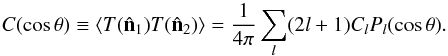 (3)Statistical
independence implies that
(3)Statistical
independence implies that 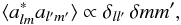 (4)and statistical isotropy
further requires that the constant of proportionality depend only on l, not
m:
(4)and statistical isotropy
further requires that the constant of proportionality depend only on l, not
m: 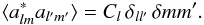 (5)The constant
 (6)is
the angular power of the multipole l.
(6)is
the angular power of the multipole l.
To properly calculate the CMB angular correlation function, one must first navigate through a complex array of processes generating the incipient fluctuations Δρ in density, followed by a comparably daunting collection of astrophysical effects, all subsumed together into multiplicative factors known as “transfer functions”, that relate the power spectrum P(κ) of the gravitational potential resulting from Δρ to the output CMB temperature fluctuations ΔT. A detailed calculation of this kind can take weeks or even months to complete, even on advanced computer platforms.
Fluctuations produced prior to decoupling lead to “primary” anisotropies, whereas those
developing as the CMB propagates from the surface of last scattering to the observer are
“secondary”. The former include temperature variations associated with photon propagation
through fluctuations of the metric. Known as the Sachs-Wolfe effect (Sachs & Wolfe
1967), this process produces fluctuations in
temperature given roughly as  (7)where ΔΦ is a
fluctuation in the gravitational potential. The Sachs-Wolfe effect is dominant on large
scales (i.e., θ ≫ 1°).
(7)where ΔΦ is a
fluctuation in the gravitational potential. The Sachs-Wolfe effect is dominant on large
scales (i.e., θ ≫ 1°).
Prior to decoupling, the plasma is also susceptible to acoustic oscillations. The density variations associated with compression and rarefaction produce baryon fluctuations resulting in a prominent acoustic peak seen at l ~ 200 in the power spectrum. Processes such as this, which depend sensitively on the microphysics, are therefore dominant on small scales, typically θ < 1°.
Once the photons decouple from the baryons, the CMB must propagate through a large scale structure with complex distributions of the gravitational potential and intra-cluster gas, neither of which is necessarily isotropic or homogeneous on small spatial scales. Astrophysical processes following recombination therefore imprint their own (secondary) signatures on the CMB temperature anisotropies. Examples of secondary processes include: the thermal and kinetic Sunyaev-Zeldovich effects (Sunyaev & Zeldovich 1980), due to inverse Compton scattering by, respectively, thermal electrons in clusters and electrons moving in bulk with their galaxies relative to the CMB “rest” frame; the integrated Sachs-Wolfe effect, induced by the time variation of gravitational potentials, and its nonlinear extension, the Rees-Sciama effect (Rees & Sciama 1968); and the deflection of CMB light by gravitational lensing. These effects are expected to produce observable temperature fluctuations at a level of order ΔT/T ~ 10-5 on arc-minute scales (though the Rees-Sciama effect typically generates much smaller fluctuations with ΔT/T ~ 10-8).
Insofar as understanding the global dynamics of the Universe is concerned, there are several reasons why we can find good value in utilizing the angular correlation function C(cosθ). This is not to say that the power spectrum (represented by the set of Cl’s) is itself not probative. On the contrary, the past forty years have shown that a meaningful comparison can now be made between theory and observations through an evaluation, or determination, of the multipole powers. But previous studies have also shown that variations caused by different cosmological parameters are not orthogonal, in the sense that somewhat similar sets of Cl’s can be found for different parameter choices (Scott et al. 1995).
A principal reason for this is that the two-point angular power spectrum emphasizes small scales (typically ~1°), making it a useful diagnostic for physics at the last scattering surface. A comparison between theory and observation on these small scales permits the precise determination of fundamental cosmological parameters, given an assumed cosmological model (Nolta et al. 2009). The two-point angular correlation function C(cosθ) contains the same information as the angular power spectrum, but highlights behavior at large angles (i.e., small values of l), the opposite of the two-point angular power spectrum. Therefore, the angular correlation function provides a better test of dynamical models driving the universal expansion.
For these reasons, we suggest that a comparison between the calculated C(cosθ) and the observations may provide a more stringent test of the assumed cosmology. The microphysical effects responsible for the high-l multipoles, featured most prominently in the power spectrum, are more likely to be generic to a broad range of expansion scenarios. But C(cosθ), which highlights the largest scale fluctuations, yields greater differentiation when it comes to the overall dynamics. A more complete discussion of the benefits of the angular power spectrum versus the angular correlation function, and vice versa, is provided in Copi et al. (2013), and many other references cited therein.
4. Angular correlation function of the CMB in ΛCDM
Let us now consider the predicted function C(cosθ) in the context of ΛCDM and its comparison to the WMAP sky. A crucial ingredient of the standard model is cosmological inflation – a brief phase of very rapid expansion from approximately 10-35 s to 10-32 s following the big bang, forcing the universe to expand much more rapidly than would otherwise have been feasible solely under the influence of matter, radiation, and dark energy, carrying causally connected regions beyond the horizon each would have had in the absence of this temporary acceleration. In ΛCDM without this exponential expansion, regions on opposite sides of the sky would not have had sufficient time to equilibrate before producing the CMB at te ~ 380 000 years after the big bang (see Melia 2013a, for a detailed explanation and a comparison between various FRW cosmologies). Therefore, the predictions of ΛCDM would be in direct conflict with the observed uniformity of the microwave background radiation, which has the same temperature everywhere, save for the aforementioned fluctuations at the level of one part in 100 000 seen in WMAP’s measured relic signal.
This required inflationary expansion drives the growth of fluctuations on all scales and predicts an angular correlation at all angles. However, as pointed out by Copi et al. (2013) in their detailed analysis of both the WMAP and Planck data, there has always been an indication (even from the older COBE-DMR observations; Hinshaw et al. 1996) that the two-point angular correlation function nearly vanishes on scales greater than about 60 degrees, contrary to what ΛCDM predicts (see Fig. 1). From this figure, one may also come away with the impression that there are significant differences between the predicted and observed angular correlation function at angles smaller than 60 degree, but because the different angular bins are correlated, the deviation between the two curves is not as statistically significant as it appears. In fact, cosmic variance from the theoretical curve (indicated by the shaded region) can essentially account for most of the disparity at these smaller angles.
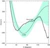 |
Fig. 1 Angular correlation function of the best-fit ΛCDM model and that inferred from the Planck SMICA full-sky map (Planck Collaboration 2013) on large angular scales. The shaded region is the one-sigma cosmic variance interval. (This figure is adapted from Copi et al. 2013.) |
A quantitative measure of the differences between the observed angular correlation function
and that predicted by ΛCDM is the so-called
S1/2 statistic introduced by the WMAP team
(Spergel et al. 2003):
 (8)A subsequent application
of this measure on the WMAP 5 year maps (Copi et al. 2009) revealed that only ~0.03% of ΛCDM model CMB skies have lower values of
S1/2 than that of the observed WMAP sky.
But we may simply be dealing with foreground subtraction issues. The final (9-year) analysis
of the WMAP data suggests that the difference between theory and observation is probably
smaller and may fall within the 1 − σ error region associated with cosmic
variance (Bennett et al. 2013).
(8)A subsequent application
of this measure on the WMAP 5 year maps (Copi et al. 2009) revealed that only ~0.03% of ΛCDM model CMB skies have lower values of
S1/2 than that of the observed WMAP sky.
But we may simply be dealing with foreground subtraction issues. The final (9-year) analysis
of the WMAP data suggests that the difference between theory and observation is probably
smaller and may fall within the 1 − σ error region associated with cosmic
variance (Bennett et al. 2013).
There are indications, however, that the differences between theory and observations may be due to more than just randomness. For example, the observed angular correlation function has a well defined shape, with a minimum at ~50°, and a relatively smooth curve on either side of this turning point. One might have expected the data points to not line up as they do within the variance window if stochastic processes were solely to blame. Moreover, one cannot ignore the fact that the observed angular correlation goes to zero beyond ~60°. Variance could have resulted in a function with a different slope than that predicted by ΛCDM, but it seems unlikely that this randomly generated slope would be close to zero above ~60°.
The recent Planck results also confirm that the S1/2 statistic is very low. In their analysis, Copi et al. (2013) find that the probability of the observed cut-sky S1/2 statistic in an ensemble of realizations of the best-fitting ΛCDM model never exceeds 0.33% for any of the analyzed combinations of maps and masks. This trend has remained intact since the release of the WMAP 3-year data. The apparent lack of temperature correlations on large angular scales is robust and increases in statistical significance as the quality of the instrumentation improves, suggesting that instrumental issues are not the cause.
If it turns out that the absence of large-angle correlation is real, and not due to cosmic variance, this may be the most significant result of the WMAP mission, because it essentially invalidates any role that inflation might have played in the universal expansion. Our principal goal in this paper is therefore to examine whether the Rh = ct Universe – a cosmology without inflation – can account for the lack of temperature correlations on large angular scales without invoking cosmic variance.
5. Angular correlation of the CMB in the Rh = ct Universe
Since the Rh = ct Universe did not undergo a
period of inflated expansion, it is not subject to the observational restriction discussed
above. Defining the density contrast
δ ≡ δρ/ρ in terms of
the density fluctuation δρ and unperturbed density ρ, we
can form the wavelike decomposition  (9)where the Fourier
component δκ depends only on cosmic time
t, and κ and r are the co-moving wavevector
and radius, respectively. In Melia & Shevchuk (2012), we derived the dynamical equation for
δκ in the
Rh = ct Universe and showed that in the
linear regime
(9)where the Fourier
component δκ depends only on cosmic time
t, and κ and r are the co-moving wavevector
and radius, respectively. In Melia & Shevchuk (2012), we derived the dynamical equation for
δκ in the
Rh = ct Universe and showed that in the
linear regime  (10)The way
perturbation growth is handled in Rh = ct,
leading to Eq. (10), is somewhat different from ΛCDM, so we will take a moment to briefly
describe the origin of this expression. As we discussed in the introduction, the chief
difference between ΛCDM and Rh = ct is that one
must guess the constituents of ρ in the former, assign an individual
equation of state to each, and then solve the growth equation derived for each of these
components separately. This is how one handles a situation in which the various species do
not necessarily feel each other’s pressure, though they do feel the gravitational influence
from the total density. The coupled equations of growth for the various components can be
quite complex, so one typically approximates the equations by expressions that highlight the
dominant species in any given era. For example, before recombination, the baryon and photon
components must be treated as a single fluid, since they are coupled by frequent
interactions in an optically-thick environment. During this period, ΛCDM assumes that “dark
energy” is smooth on scales corresponding to the fluctuation growth, and treats the
baryon-photon fluid as a single perturbed entity with the pressure of radiation and an
overall energy density corresponding to their sum. Once the radiation decouples from the
luminous matter, all four constituents (including dark matter) must be handled separately,
though in a simplified approach one may ignore the radiation, which becomes subdominant at
later times.
(10)The way
perturbation growth is handled in Rh = ct,
leading to Eq. (10), is somewhat different from ΛCDM, so we will take a moment to briefly
describe the origin of this expression. As we discussed in the introduction, the chief
difference between ΛCDM and Rh = ct is that one
must guess the constituents of ρ in the former, assign an individual
equation of state to each, and then solve the growth equation derived for each of these
components separately. This is how one handles a situation in which the various species do
not necessarily feel each other’s pressure, though they do feel the gravitational influence
from the total density. The coupled equations of growth for the various components can be
quite complex, so one typically approximates the equations by expressions that highlight the
dominant species in any given era. For example, before recombination, the baryon and photon
components must be treated as a single fluid, since they are coupled by frequent
interactions in an optically-thick environment. During this period, ΛCDM assumes that “dark
energy” is smooth on scales corresponding to the fluctuation growth, and treats the
baryon-photon fluid as a single perturbed entity with the pressure of radiation and an
overall energy density corresponding to their sum. Once the radiation decouples from the
luminous matter, all four constituents (including dark matter) must be handled separately,
though in a simplified approach one may ignore the radiation, which becomes subdominant at
later times.
The situation in Rh = ct is quite different for several reasons. First of all, the overall equation of state in this cosmology is not forced on the system by the constituents; it is the other way around. The symmetries implied by the Cosmological Principle and Weyl’s postulate together, through the application of general relativity, only permit a constant expansion rate, which means that p = −ρ/3. The expansion rate depends on the total energy density, but not on the partitioning among the various constituents. Instead, the constituents must partition themselves in such a way as to always guarantee that this overall equation of state is maintained during the expansion.
And since the pressure is therefore a non-negligible fraction of ρ at all times, one cannot use the equations of growth derived from Newtonian theory (commonly employed in ΛCDM), since p itself acts a source of curvature. One must therefore necessarily start with the relativistic growth equation (numbered 41 in Melia & Shevchuk 2012), which correctly incorporates all of the contributions from ρ and p. This equation is ultimately derived from Einstein’s field equations using the perfect-fluid form of the stress-energy tensor, written in terms of the total ρ and total p, but without specifying the subpartitioning of the density and pressure among the various constituents. With this approach, there is only one growth equation.
On occasion, it is also necessary to use the relativistic growth equation in ΛCDM. But there, one typically chooses a regime where a single constituent is dominant, say during the matter-dominated era, and then one assumes that ρ is essentially just the density due to matter (for which also p ≈ 0). But in general, since the pressure appearing in the stress-energy tensor is the total pressure, one cannot mix and match different components that may or may not “feel” each other’s influence (as described above). So in fact using the relativistically correct growth equation is difficult in ΛCDM, unless one can make suitable approximations in a given regime.
In Rh = ct, on the other hand, the total pressure is always −ρ/3, so the key question is whether all of the constituents participate in the perturbation growth, or whether only some of them do. There is no doubt that the baryons and photons are coupled prior to recombination. In ΛCDM, one assumes that dark energy is coupled only weakly, acting as a smooth background. In Rh = ct, dark energy cannot be a cosmological constant. One therefore assumes that during the early fluctuation growth, everything is coupled strongly in order to maintain the required total pressure −ρ/3.
In short, there is one assumption made in each cosmology. In ΛCDM, dark energy is a cosmological constant that remains smooth while the baryon-photon fluid is perturbed at early times. In Rh = ct, dark energy cannot be a cosmological constant, and everything is coupled strongly at early times, so the perturbation affects the total energy density ρ. One must always use the correct relativistic growth equation, which includes p as a source of gravity.
In the end, this equation simplifies considerably because the active mass in
Rh = ct is proportional to
ρ + 3p = 0, and therefore the gravitational term
normally appearing in the standard model is absent. But this does not mean that
δκ cannot grow. Instead, because
p < 0, the (usually dissipative) pressure term on
the right-hand-side here becomes an agent of growth. Moreover, there is no Jeans length
scale. In its place is the gravitational radius, which we can see most easily by recasting
this differential equation in the form
 (11)where
 (12)Note, in particular, that
both the gravitational radius Rh and the fluctuation scale
λ vary with t in exactly the same way, so
Δκ is therefore a constant in time. But the growth rate of
δκ depends critically on whether
λ is less than or greater than
2πRh.
(12)Note, in particular, that
both the gravitational radius Rh and the fluctuation scale
λ vary with t in exactly the same way, so
Δκ is therefore a constant in time. But the growth rate of
δκ depends critically on whether
λ is less than or greater than
2πRh.
The fact that Rh = ct does not have a Jeans length is itself quite relevant to understanding the observed lack of any scale dependence in the measured matter correlation function (Watson et al. 2011). As one can see from the general form of the dynamical equation for δκ (Melia & Shevchuk 2012), only a cosmology with p = −ρ/3 has this feature. In every other case, both the pressure and gravitational terms are present in Eq. (10), which always produces a Jeans scale. For example, ΛCDM predicts different functional forms for the matter correlation function on different spatial scales, and is therefore not consistent with the observed matter distribution.
A simple solution to Eq. (11) is the power law
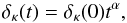 (13)where evidently
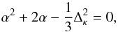 (14)so that
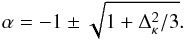 (15)Thus, for small
fluctuations (λ ≪ 2πRh), the
growing mode is
(15)Thus, for small
fluctuations (λ ≪ 2πRh), the
growing mode is 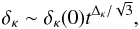 (16)whereas for large
fluctuations
(λ > 2πRh),
the dominant mode
(16)whereas for large
fluctuations
(λ > 2πRh),
the dominant mode  (17)does not even grow. For
both small and large fluctuations, the second mode decays away.
(17)does not even grow. For
both small and large fluctuations, the second mode decays away.
A quick inspection of the growth rate implied by Eq. (16) reveals that the fluctuation
spectrum must have entered the nonlinear regime well before recombination (which presumably
occurred at te ~ 104–105 years).
Therefore, without carrying out a detailed simulation of the fluctuation growth at early
times, it is not possible to extract the power spectrum
 (18)unambiguously. Fortunately,
this is not the key physical ingredient we are seeking. Instead, the central question is
“What is the maximum range over which the fluctuations would have grown, either linearly or
nonlinearly, prior to recombination?” and this we can answer rather straightforwardly.
(18)unambiguously. Fortunately,
this is not the key physical ingredient we are seeking. Instead, the central question is
“What is the maximum range over which the fluctuations would have grown, either linearly or
nonlinearly, prior to recombination?” and this we can answer rather straightforwardly.
Equations (16) and (17) suggest that – without inflation – the maximum fluctuation size at
any given time t was
λmax(t) ~ 2πRh(t).
In the Rh = ct Universe, the comoving distance
to the last scattering surface (at time te) is
 (19)Therefore, the maximum
angular size θmax of any fluctuation associated with the CMB
emitted at te has to be
(19)Therefore, the maximum
angular size θmax of any fluctuation associated with the CMB
emitted at te has to be
 (20)where
 (21)is
the proper distance to the last scattering surface at time te.
That is,
(21)is
the proper distance to the last scattering surface at time te.
That is,  (22)Thus, if we naively
adopt the times t0 = 13.7 Gyr and
te ≈ 380 000 yrs from the standard model, we find that
θmax ~ 34°. As we shall see, it is the existence of
this limit, more than any other aspect of the CMB anisotropies in the
Rh = ct Universe, that accounts for the shape
of the observed angular correlation function in Fig. 1.
(22)Thus, if we naively
adopt the times t0 = 13.7 Gyr and
te ≈ 380 000 yrs from the standard model, we find that
θmax ~ 34°. As we shall see, it is the existence of
this limit, more than any other aspect of the CMB anisotropies in the
Rh = ct Universe, that accounts for the shape
of the observed angular correlation function in Fig. 1.
Since we are here beginning to identify specific values for the age of the Universe t0, and the recombination time te, both of which impact observables, such as θmax, it is important to remind ourselves that the concordance values of the ΛCDM parameters render the expansion history in the standard model so similar to that in Rh = ct that today we measure Rh(t0) ≈ ct0. In other words, the age of the concordance ΛCDM Universe is virtually identical to that of the Rh = ct Universe, so using t0 = 13.7 Gyr for these estimates is quite reasonable.
Insofar as the radiation in Rh = ct is concerned, its temperature increases inversely with a(t), as it does in ΛCDM, so there is little difference in the radiation fields within these two cosmologies. What does differ is the dark-energy content and its equation of state. In ΛCDM, one typically makes the simplest assumption, which is that dark energy is a cosmological constant and therefore becomes less important as t → 0. In Rh = ct, on the other hand, all that matters is that the constituents together must contribute an overall equation of state p = −ρ/3, so any components other than matter and radiation have a stronger dependence on a(t) (and therefore t) than they do in ΛCDM. However, the radiation will still have the same temperature at a given value of a(t) as it does in ΛCDM. This suggests that the range over which te will fall in Rh = ct is probably not far from 380 000 yrs. Below, we will consider the impact on C(cosθ) from changes to the ratio t0/te over the range 5 × 10⁴−5 × 10⁶ (see Fig. 4).
In this paper, we wish to identify the key elements of the theory responsible for the shape
of C(cosθ), without necessarily getting lost in the
details of the complex treatment alluded to in Sect. 3 above, so we will take a simplified
approach used quite effectively in other applications (Efstathiou 1990). For example, we will ignore the transfer function, and consider
only the Sachs-Wolfe effect, since previous work has shown that this is dominant on scales
larger than ~1°. From a practical standpoint, this approximation affects the
shape of C(cosθ) closest to θ = 0 in Fig.
1, but that’s not where the most interesting comparison with the data will be made. We will
also adopt a heuristic, Newtonian argument to establish the scale-dependence of this effect,
noting that  (23)where
 (24)Thus, from Eq. (7), we see
that
(24)Thus, from Eq. (7), we see
that  (25)But the variance in density
over a particular comoving scale λ is given as
(25)But the variance in density
over a particular comoving scale λ is given as
 (26)(Efstathiou
1990). Not knowing the exact form of the power
spectrum emerging from the nonlinear growth prior to recombination, we will parametrize it
as follows,
(26)(Efstathiou
1990). Not knowing the exact form of the power
spectrum emerging from the nonlinear growth prior to recombination, we will parametrize it
as follows,  (27)where the (unknown)
constant b is expected to be ~O(1).
(27)where the (unknown)
constant b is expected to be ~O(1).
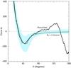 |
Fig. 2 Angular correlation function of the CMB in the Rh = ct Universe, for b = 3 and t0/te = 5 × 10⁵ (see text). The Planck data are the same as those shown in Fig. 1. The shaded region is the one-sigma cosmic variance interval. |
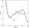 |
Fig. 3 Angular correlation function of the CMB in the Rh = ct Universe, for b = 3 and t0/te = 5 × 10⁵, together with the best-fit ΛCDM model, compared with the Planck data. |
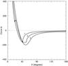 |
Fig. 4 Impact on the angular correlation function C(cosθ) in the Rh = ct Universe from a change in the ratio t0/te: (Curve 1), 5 × 10⁶; (Curve 2), 5 × 10⁵; (Curve 3), 5 × 10⁴. |
This form of P(κ) is based on the following reasoning. The conventional procedure is to assume a scale-free initial power-law spectrum, which we also do here. In ΛCDM, these fluctuations grow and then expand to all scales during the required inflationary phase. In Rh = ct, the fluctuation growth is driven by the (negative) pressure, represented by the term on the right-hand side of Eq. (10). Very importantly, because there is no Jeans length, fluctuations can in principle grow on all scales. However, this equation also shows that what matters most is the ratio of the fluctuation length λ to the gravitational radius Rh(t) at time t. The solution to this equation shows that only fluctuations with λ < 2πRh will grow, and that those modes that grow, will grow rapidly, given their strong dependence on t (see Eq. (16)).
The most important result we get from this analysis is that fluctuations will grow quickly in amplitude until they get to the size 2πRh(t), and then the growth stops. In ΛCDM, on the other hand, growth continues due to inflation. The simple parametrization in Eq. (27) incorporates these essential effects: first, the initial seed spectrum is assumed to be scale-free, which means that P(κ) ~ κ. Since the growth rate depends critically on the ratio Rh/λ, one would expect P(κ) to be dominated by the smaller wavelengths (i.e., the larger κ’s), and be altered more and more for increasing wavelengths (i.e., smallter κ’s). Thus, for large κ, P(κ) should still go roughly as κ. However, for smaller κ, the growth rate decreases with decreasing κ, so one would expect a greater and greater depletion in power with decreasing κ. The second term in Eq. (27) represents this effect.
Having said this, the key physical element most responsible for the shape of the angular correlation function is the ratio t0/te, since this determines the size of the gravitational horizon Rh(te) from which one determines the maximum angle θmax of the fluctuations. The b in the parametrization of Eq. (27) affects the location of the minimum in (and value of) C(cosθ), but not qualitatively, as exhibited by the variations shown in Fig. 5. Since the results are only weakly dependent on b, the parametrization in Eq. (27) does not appear to be overly influencing our results.
It is not difficult to see from Eqs. (26) and (27) that δρ is therefore
given as 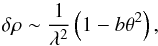 (28)where the definition of
θ is analogous to that of θmax in Eq. (20).
Thus, the amplitude of the Sachs-Wolfe temperature fluctuations follows the very simple form
(28)where the definition of
θ is analogous to that of θmax in Eq. (20).
Thus, the amplitude of the Sachs-Wolfe temperature fluctuations follows the very simple form
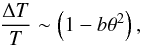 (29)but only up to the
maximum angle θmax established earlier. The CMB angular
correlation function C(cosθ) calculated using Eq. (29) is
shown in Fig. 2, together with the Planck data (Planck Collaboration 2013), for b = 3 and
t0/te = 5 × 10⁵.
To facilitate a comparison between all three correlation functions (from
Planck, ΛCDM, and Rh = ct),
we show them side by side in Fig. 3.
(29)but only up to the
maximum angle θmax established earlier. The CMB angular
correlation function C(cosθ) calculated using Eq. (29) is
shown in Fig. 2, together with the Planck data (Planck Collaboration 2013), for b = 3 and
t0/te = 5 × 10⁵.
To facilitate a comparison between all three correlation functions (from
Planck, ΛCDM, and Rh = ct),
we show them side by side in Fig. 3.
We are not yet in a position to calculate the probability of getting the observed S1/2 for all possible realizations of the Rh = ct Universe, because our estimation of the fluctuation spectrum in this cosmology is still at a very rudimentary stage. Our calculation of the correlation function is based solely on the Sachs-Wolfe effect, which dominates at large angles. However, the general agreement between theory and observation in Figs. 2 and 3 suggests that the angular correlation function associated with an FRW cosmology without inflation (such as Rh = ct) matches that observed with WMAP and Planck qualitatively better than ΛCDM. For example, we note from Fig. 3 that Rh = ct does a better job predicting the location of the minimum, θmin, the value of C(cosθmin) at this angle and, particularly, the lack of significant angular correlation at angles θ > 60°.
Of course, one should wonder how sensitively any of these results depends on the chosen values of b and t0/te. The short answer is that the dependence is weak, in part because the ratio t0/te enters into the calculation only via its log (see Eq. (22)). Figure 4 illustrates the impact on C(cosθ) of changing the value of t0/te, from 5 × 10⁶ (curve 1), to 5 × 10⁵ (curve 2), and finally to 5 × 10⁴ (curve 3).
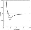 |
Fig. 5 Impact on the angular correlation function C(cosθ) in the Rh = ct Universe from a change in the value of b: (Curve 1), b = 2; (Curve 2), b = 3; (Curve 3), b = 4. |
The dependence of these results on the value of b is illustrated in Fig. 5, which shows the curves corresponding to b = 2 (curve 1), b = 3 (curve 2), and b = 4 (curve 3). In all cases, the overarching influence is clearly the existence of θmax, which cuts off any angular correlation at angles greater than ~60°. We would argue that any of the curves in Figs. 3 and 4 present a better match to the WMAP data than the ΛCDM curve shown in Fig. 1. Therefore, the difference between ΛCDM and the data may be due to inflation rather than cosmic variance.
Finally, let us acknowledge the fact that although ΛCDM may not appear to provide the better explanation for the angular correlation function, it nonetheless does extremely well in accounting for the observed angular power spectrum for l > 20 (see, e.g., Bennett et al. 2013; Planck Collaboration 2013). Along with its remarkable fit to the Type Ia SN data, this has been arguably the biggest success story of this long-standing cosmological model. We have not yet included all of the physical effects, such as baryon acoustic oscillations, occurring near the surface of last scattering in the Rh = ct scenario, so it is not yet possible to carry out a complete comparative analysis of the entire power spectrum between the two models, certainly not for l > 10−20. The work of Scott et al. (1995), among others, suggests that, unlike the Sachs-Wolfe effect, which is quite sensitive to the expansion dynamics, the local physics where the CMB is produced may be generic to a wide range of evolutionary histories. So the fact that ΛCDM does not acccount very well for the angular correlation function, which tends to highlight features predominantly at large angles (θ > 1−10 degrees), is not inconsistent with the reality that it fits the high-l angular power spectrum very well.
To demonstrate how these two approaches to the analysis of angular information in the CMB focus on quite different aspects of the fluctuation problem, we show in Fig. 6 the angular power spectrum produced solely by the Sachs-Wolfe effect in the Rh = ct Universe. This fit for l < 10−20 is actually a better match to the observations than that associated with ΛCDM, but what is lacking, of course, is information for l > 10−20, where the standard model does exceptionally well. It is comforting to see that the qualitatively good fit exhibited by Rh = ct in Figs. 2 and 3, is confirmed by the very good fit also seen in the angular power spectrum (Fig. 6) at low values of l. (The details of how this angular power spectrum is calculated are provided in a companion paper, whose principal goal is to discuss the apparent low-multipole alignment in the CMB; see Melia 2012.) Future work must include a more complete analysis than we have presented here, to approach the extraordinary level of detail now available in applications of the standard model.
 |
Fig. 6 Theoretical CMB power spectrum due solely to Sachs-Wolfe-induced fluctuations in the Rh = ct Universe (solid, thick curve), in comparison with the power spectrum measured from the full WMAP sky (thin, jagged line; Spergel et al. 2003; Tegmark et al. 2003). The gray region represents the one-sigma uncertainty. The power spectrum for l > 10−20 is dominated by small-scale physical effects, such as baryon acoustic oscillations near the surface of last scattering, which are not included in our analysis. For comparison, we also show the WMAP best-fit (dashed) curve, calculated with all of the physical effects producing the fluctuations. This curve fits the data very well, particularly at very high l’s, corresponding to fluctuations on scales smaller than ~10°. |
6. Conclusions
It is essential for us to identify the key physical ingredient that guides the behavior of a diagnostic as complicated as C(cosθ) in Figs. 1 through 5. An episode of inflation early in the Universe’s history would have driven all fluctuations to grow, whether in the radiation dominated era, or later during the matter dominated expansion, to very large opening angles, producing a significant angular correlation on all scales. The Planck data reproduced in Fig. 1 (and also the earlier WMAP observations) show that this excessive expansion may not have occurred, if the difference between theory and observations is not due solely to cosmic variance. In the Rh = ct Universe, on the other hand, there was never any inflationary expansion (Melia 2013a), so there was a limit to how large the fluctuations could have grown by the time (te) the CMB was produced at the surface of last scattering. This limit was attained when fluctuations of size λ/2π had reached the gravitational horizon Rh(te). And for a ratio t0/te ~ 35 000–40 000, this corresponds to a maximum fluctuation angle θmax ~ 30–35°. This limit is the key ingredient responsible for the shape of the angular correlation function seen in Figs. 2–5. Though other influences, such as Doppler shifts, the growth of adiabatic perturbations, and the integrated Sachs-Wolfe effect, have yet to be included in these calculations, they are not expected – on the basis of previous work – to be dominant; they would modify the shape of C(cosθ) only slightly (perhaps even bringing the theoretical curve closer to the data). The positive comparison between the observed and calculated C(cosθ) curves seen in these figures offers some support to the viability of the Rh = ct Universe as the correct description of nature.
One might also wonder whether the observed lack of angular correlation and the alignment of quadrupole and octopole moments are somehow related. This question was the subject of Rakić & Schwarz’s analysis (Rakić & Schwarz 2007), which concluded that the answer is probably no. More specifically, they inferred that having one does not imply a larger or smaller probability of having the other. However, this analysis was rather simplistic, in the sense that it did not consider whether alternative cosmologies, such as the Rh = ct Universe, could produce the observed alignment as a result of the ~Rh(te) (noninflated) fluctuation-size limit, in which case the two anomalies would in fact be related, though only indirectly.
In related work, it was shown by Sarkar et al. (2011) that there is no statistically significant correlation in ΛCDM between the missing power on large angular scales and the alignment of the l = 2 and l = 3 multipoles. If not due to variance, the inconsistency between the standard model and the WMAP data may therefore be greater than each of the anomalies alone, because their combined statistical significance is equal to the product of their individual significances. As pointed out by Sarkar et al. (2011), such an outcome would require a causal explanation.
In this paper, we have shown that at least one of these anomalies is not generic to all FRW cosmologies. In fact, the observed angular correlation function is a good match to that predicted in the Rh = ct Universe. This property of the CMB might be pointing to the existence of a maximum angular size θmax for the large-scale fluctuations, imposed by the gravitational horizon Rh at the time te of last scattering.
Acknowledgments
This research was partially supported by ONR grant N00014-09-C-0032 at the University of Arizona, and by a Miegunyah Fellowship at the University of Melbourne. I am particularly grateful to Amherst College for its support through a John Woodruff Simpson Lectureship. And I am happy to acknowledge the helpful comments by the anonymous referee, that have led to a significant improvement in this manuscript.
References
- Bennett, C. L., Hill, R. S., Hinshaw, G., et al. 2003, ApJS, 148, 97 [NASA ADS] [CrossRef] [Google Scholar]
- Bennett, C. L., Larson, D., Weiland, J. L., et al. 2013, ApJS, 208, 20 [Google Scholar]
- Copi, C. J., Huterer, D., Schwarz, D. J., & Starkman, G. D. 2009, MNRAS, 399, 295 [NASA ADS] [CrossRef] [Google Scholar]
- Copi, C. J., Huterer, D., Schwarz, D. J., & Starkman, G. D. 2013, MNRAS, submitted [arXiv:1310.3831] [Google Scholar]
- Efstathiou, G. 1990, in Physics of the Early Universe, eds. J. A. Peacock, A. F. Heavens, & A. T. Davies (Edinburgh: SUSSP) [Google Scholar]
- Guth, A. H. 1981, Phys. Rev. D, 23, 347 [NASA ADS] [CrossRef] [MathSciNet] [Google Scholar]
- Hinshaw, G., Branday, A. J., Bennett, C. L., et al. 1996, ApJ, 464, L25 [NASA ADS] [CrossRef] [Google Scholar]
- Linde, A. 1982, Phys. Lett. B, 108, 389 [Google Scholar]
- Melia, F. 2007, MNRAS, 382, 1917 [NASA ADS] [CrossRef] [Google Scholar]
- Melia, F. 2012, MNRAS, submitted [arXiv:1207.0734] [Google Scholar]
- Melia, F. 2013a, A&A, 553, A76 [NASA ADS] [CrossRef] [EDP Sciences] [Google Scholar]
- Melia, F. 2013b, Phys. Lett. B, submitted [Google Scholar]
- Melia, F. 2013c, CQG, 30, 155007 [NASA ADS] [CrossRef] [Google Scholar]
- Melia, F., & Abdelqader, M. 2009, IJMP-D, 18, 1889 [NASA ADS] [CrossRef] [Google Scholar]
- Melia, F., & Maier, R. S. 2013, MNRAS, 432, 2669 [NASA ADS] [CrossRef] [Google Scholar]
- Melia, F., & Shevchuk, A. 2012, MNRAS, 419, 2579 [NASA ADS] [CrossRef] [Google Scholar]
- Moresco, M., Verde, L., Pozzetti, L., Jimenez, R., & Cimatti, A. 2012, JCAP, 07, 053 [Google Scholar]
- Nolta, M. R., Dunkley, J., Hill, R. S., et al. 2009, ApJS, 180, 296 [NASA ADS] [CrossRef] [Google Scholar]
- Planck Collaboration 2013, A&A, submitted [arXiv:1303.5075] [Google Scholar]
- Rakić, A., & Schwarz, D. J. 2007, Phys. Rev. D, 75, 103002 [NASA ADS] [CrossRef] [Google Scholar]
- Rees, M. J., & Sciama, D. W. 1968, Nature, 217, 511 [NASA ADS] [CrossRef] [Google Scholar]
- Sachs, R. K., & Wolfe, A. M. 1967, ApJ, 147, 73 [NASA ADS] [CrossRef] [Google Scholar]
- Sarkar, D., Huterer, D., Copi, C. J., Starkman, G. D., & Schwarz, D. J. 2011, Astropart. Phys., 34, 591 [NASA ADS] [CrossRef] [Google Scholar]
- Scott, D., Silk, J., & White, M. 1995, Science, 268, 829 [NASA ADS] [CrossRef] [PubMed] [Google Scholar]
- Spergel, D. N., Verde, L., Peiris, H. V., et al. 2003, ApJS, 148, 175 [NASA ADS] [CrossRef] [Google Scholar]
- Sunyaev, R. A., & Zeldovich, I. B. 1980, MNRAS, 190, 413 [NASA ADS] [CrossRef] [Google Scholar]
- Tegmark, M., de Oliveira-Costa, A., & Hamilton, A. J., 2003, Phys. Rev. D, 68, 123523 [NASA ADS] [CrossRef] [Google Scholar]
- Wright, E. L., Bennett, C. L., Gorski, K., Hinshaw, G., & Smoot, G. F. 1996, ApJ, 464, L21 [NASA ADS] [CrossRef] [Google Scholar]
- Watson, D. F., Berlind, A. A., & Zentner, A. R. 2011, ApJ, 738, 22 [NASA ADS] [CrossRef] [Google Scholar]
- Wei, J.-J., Wu, X., & Melia, F. 2013, ApJ, 772, 43 [NASA ADS] [CrossRef] [Google Scholar]
All Figures
|
Fig. 1 Angular correlation function of the best-fit ΛCDM model and that inferred from the Planck SMICA full-sky map (Planck Collaboration 2013) on large angular scales. The shaded region is the one-sigma cosmic variance interval. (This figure is adapted from Copi et al. 2013.) |
| In the text | |
|
Fig. 2 Angular correlation function of the CMB in the Rh = ct Universe, for b = 3 and t0/te = 5 × 10⁵ (see text). The Planck data are the same as those shown in Fig. 1. The shaded region is the one-sigma cosmic variance interval. |
| In the text | |
|
Fig. 3 Angular correlation function of the CMB in the Rh = ct Universe, for b = 3 and t0/te = 5 × 10⁵, together with the best-fit ΛCDM model, compared with the Planck data. |
| In the text | |
|
Fig. 4 Impact on the angular correlation function C(cosθ) in the Rh = ct Universe from a change in the ratio t0/te: (Curve 1), 5 × 10⁶; (Curve 2), 5 × 10⁵; (Curve 3), 5 × 10⁴. |
| In the text | |
|
Fig. 5 Impact on the angular correlation function C(cosθ) in the Rh = ct Universe from a change in the value of b: (Curve 1), b = 2; (Curve 2), b = 3; (Curve 3), b = 4. |
| In the text | |
|
Fig. 6 Theoretical CMB power spectrum due solely to Sachs-Wolfe-induced fluctuations in the Rh = ct Universe (solid, thick curve), in comparison with the power spectrum measured from the full WMAP sky (thin, jagged line; Spergel et al. 2003; Tegmark et al. 2003). The gray region represents the one-sigma uncertainty. The power spectrum for l > 10−20 is dominated by small-scale physical effects, such as baryon acoustic oscillations near the surface of last scattering, which are not included in our analysis. For comparison, we also show the WMAP best-fit (dashed) curve, calculated with all of the physical effects producing the fluctuations. This curve fits the data very well, particularly at very high l’s, corresponding to fluctuations on scales smaller than ~10°. |
| In the text | |
Current usage metrics show cumulative count of Article Views (full-text article views including HTML views, PDF and ePub downloads, according to the available data) and Abstracts Views on Vision4Press platform.
Data correspond to usage on the plateform after 2015. The current usage metrics is available 48-96 hours after online publication and is updated daily on week days.
Initial download of the metrics may take a while.