| Issue |
A&A
Volume 560, December 2013
|
|
|---|---|---|
| Article Number | A17 | |
| Number of page(s) | 5 | |
| Section | Planets and planetary systems | |
| DOI | https://doi.org/10.1051/0004-6361/201322272 | |
| Published online | 29 November 2013 | |
X-ray irradiation and mass-loss of the hot Jupiter WASP-43b
Hamburger Sternwarte, Universität Hamburg, Gojenbergsweg 112, 21029 Hamburg, Germany
e-mail: stefan.czesla@hs.uni-hamburg.de
Received: 12 July 2013
Accepted: 29 October 2013
We report the X-ray detection of the low-mass K7V star WASP-43, which is orbited by a hot Jupiter in one of the closest exoplanet orbits known to date. The high mean density of the planet implies a massive core with ≈130 M⊕, yielding a heavy-element mass-fraction of 20%. From an 18 ks long XMM-Newton observation, we derive an X-ray luminosity of 6.7+3.5-3.3 × 1027 ergss-1, which puts WASP-43 among the active K-stars, which is compatible with its relatively young age derived in previous studies. The X-ray luminosity translates into a soft X-ray flux of (10.2 ± 5.4) × 103 erg cm-2 s-1 at the substellar point. According to our modeling, the combined X-ray and extreme ultraviolet flux may trigger mass-loss at a rate of up to ≈1012 gs-1 via energy-limited atmospheric escape. We infer that it is unlikely that the planet has lost more than 2.5% of its current mass through that channel and that activity-induced mass-loss has not substantially altered its evolution.
Key words: stars: activity / stars: coronae / planetary systems / stars: individual: WASP-43 / X-rays: stars
© ESO, 2013
1. Introduction
While dozens of hot Jupiters have been detected to date, only a small minority of them orbit low-mass K- and M-stars. A particularly interesting case is the WASP-43 system, consisting of a low-mass K7V-type host star and the hot Jovian planet WASP-43b (Hellier et al. 2011). Today, only a single hot Jupiter is known to orbit an even less massive star, namely, the 0.59 M⊙ M-star KOI-254 (Johnson et al. 2012). Yet, with a semi-major axis of 0.015 AU, WASP-43b remains the most closely orbiting hot Jupiter known1. WASP-43b has a circular orbit and transits its host star every 0.81 d (Hellier et al. 2011; Gillon et al. 2012). With about the same size as Jupiter and twice its mass, it also shows twice the mean Jovian density (see Table 1).
Although WASP-43b orbits its host star exceptionally closely, Hellier et al. (2011) showed that the system geometry is not at all exceptional when it is expressed in terms of the stellar Roche radius, which is also small as a result of the low stellar mass. The same authors found that WASP-43b orbits at 2.1 Roche radii, which is compatible with the scenario of orbital circularization after third-body interaction and, indeed, not unusual for hot Jupiters. According to Hellier et al. (2011), the “main novelty contributed by WASP-43b is that, at K7, the host star is of much later spectral type than the other stars hosting planets with apparently short tidal lifetimes”. Furthermore, it was argued that the rarity of hot Jupiters around low-mass stars such as WASP-43 either indicates that they cannot be observed because of their short lifetimes or that such planets rarely form around low-mass stars – a suggestion with some support from theory (Laughlin et al. 2004).
Furthermore, Gillon et al. (2012) argued that the high density and strong irradiation of WASP-43b favor a massive core. Their infrared transit-photometry indicates a poor energy redistribution from the day- to the night-side. This result is confirmed by the secondary eclipse measurements in the H- and K-band obtained by Wang et al. (2013), who determined that ≲15 − 25% of the day-side energy is redistributed to the night-side.
Stellar and planetary parameters of the WASP-43 system.
Based on photometric variability, Hellier et al. (2011) determined a value of 15.6 d for the rotation period of the host star WASP-43, which translates into a vsin(i) value of 2 km s-1 given the canonical radius of a K7V star. The same authors derived a gyrochronological age estimate of 400 Ma, which is compatible with a nondetection of lithium and the presence of strong Ca II H and K emission-line cores, showing that the star is active. Hellier et al. (2011) noted, however, that the star may be older if it has been spun up through tidal interaction with its planet.
Magnetic activity is ubiquitous among late-type stars (e.g., Schmitt & Liefke 2004). Energy stored in magnetic fields and released in the upper stellar atmosphere is thought to power the bulk of stellar extreme ultraviolet and X-ray emission. This high-energy radiation can efficiently be absorbed in planetary atmospheres, where the additional heating leads to atmospheric expansion and, eventually, the formation of a planetary wind, which in turn results in mass loss (Lammer et al. 2003). Planets exposed to extreme high-energy bombardment, such as CoRoT-2b and CoRoT-7b, are thought to experience mass-loss at rates on the order of 1011−1013 gs-1 (e.g., Schröter et al. 2011; Poppenhaeger et al. 2012). It has even been proposed that activity-induced mass-loss can strip the entire gaseous envelope from a Jovian planet to leave behind no more than its solid core (Jackson et al. 2010).
While being transparent in the optical, the suspected extended atmospheres of hot Jupiters are opaque – and therefore detectable – at X-ray wavelengths. The first successful such observation has been reported on by Poppenhaeger et al. (2013), who detected the X-ray transit of the hot Jupiter HD 189733b. According to their modeling, the transit is about three times deeper in X-rays than in the optical, which makes the effective X-ray radius of the planet 75% larger than its optical counterpart. In the cases of CoRoT-2b and CoRoT-7b, the measured X-ray luminosities of the host stars suggest an even stronger dose of extreme ultraviolet (EUV) and X-ray irradiation than that experienced by HD 189733b (Schröter et al. 2011; Poppenhaeger et al. 2012). Similar observations in more system will be extremely helpful in constraining planetary evaporation and mass-loss and, therefore, the early evolution of planetary systems.
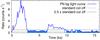 |
Fig. 1 High-energy PN light curve (10 − 12 keV, 100 s binning). The horizontal lines indicate the default (0.4 cts-1, dotted) and 2.5 times elevated (1 cts-1, dashed) cut-offs. The good-time intervals for the elevated cut-off are indicated by the shading. |
2. Observations and data analysis
On May 11, 2012, XMM-Newton observed WASP-43 for about 18 ks (Observation ID 0694550101). We reduced the data using the Science Analysis Software (SAS 12.0.1) following standard reduction procedures. The two MOS instruments and the PN camera were operated in full-frame mode using the thin filter. Our analysis shows that optical loading does not affect the observations.
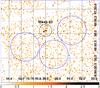 |
Fig. 2 PN image of WASP-43 (0.2 − 2 keV band). The labeled black circle depicts the source region, the larger blue regions are used for background extraction. |
The data are heavily affected by strong and variable background contamination. In Fig. 1 we show the high-energy (10 − 12 keV) light curve obtained with the PN. The first three kilo-seconds of the observation are affected by a particularly pronounced background flare, which is followed by a number of less severe high-energy events. We note that the data cover a secondary transit, which is irrelevant for the analysis, however.
The recommended cut-off rates for background filtering are 0.35 counts s-1 in the >10 keV band for the MOS and 0.4 counts s-1 in the 10−12 keV band for the PN2. As these cut-offs leave too few good-time-intervals for the PN, we experimented with different filtering choices and found consistent results for the derived source fluxes. To become independent of the specific filtering choice, we decided to employ an algorithm that allows for variations in background without loosing sensitivity in source flux.
2.1. Source detection and count-rate
From the filtered event files, we extracted the source counts based on a circular region placed on the nominal position of WASP-43. Our extraction region has a radius of 15′′ and, therefore, covers about 70% of the point spread function. The background was measured in several circular regions located in source-free sections of the same CCD close to WASP-43 (see Fig. 2). Table 2 lists the number of photons in the source region, the expected number of background photons therein, and the resulting net count-rate using the recommended standard filtering, 2.5 times the standard background cut-offs, and applying no time-filtering at all.
To accurately account for the strong background variability, we derived a maximum-likelihood estimate for the source count-rate. In particular, we constructed a source- and a background-region light curve with ns,i and nb,i counts in the ith time bin. Assuming a constant source count-rate, s0, the expectation value, λi, for ns,i becomes  (1)where Δti is the length of the ith bin and w is the area ratio between source and background region. Here, we imply that the background expectation value has been accurately determined using a large background region. In practice, we assumed that the total background density in the source region is the same as that in the background region and that the temporal evolution of the background varies with the total 10 − 12 keV detector count-rate for the PN data and >10 keV for the MOS data. Then, Poisson statistics yields the likelihood
 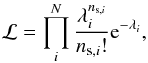 (2)and, therefore,
 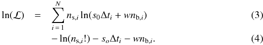 The maximum-likelihood estimate of the source count-rate was determined by finding the root of the equation
 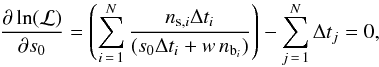 (5)which can be solved by iteration. Limiting the analysis to the 0.2 − 2 keV band, where we expect the peak of stellar X-ray emission, we determined a net source count-rate of (4 ± 0.7) ct ks-1 in the PN, (1.2 ± 0.3) ct ks-1 in MOS1, and (1.1 ± 0.3) ct ks-1 in MOS2, which yields a total XMM-Newton count-rate of (6.3 ± 0.8) ct ks-1 in all three detectors.
The derived net source count-rates do not depend on the applied filtering cut-off and are mutually consistent also with the maximum-likelihood estimate. An X-ray source at the position of WASP-43 is detected with a significance higher than 99%.
2.2. Spectral analysis
Our spectral analysis is based on the event files generated with 2.5 times the default cut-offs, which provide a good compromise between background contamination and available time (cf., Fig. 1). The individual MOS spectra were added using the mathpha tool of the SAS, which takes the different effective areas and exposure times into account.
Source count-rate as a function of background filtering cut-offs in the 0.2 − 2.0 keV band.
We grouped the spectra such that each spectral bin comprised five counts, resulting in a variable bin width (see Fig. 3). Using XSPEC V12.6.0 (Arnaud 1996), we fit an absorbed one-temperature APEC model (Foster et al. 2012) with solar abundances (Grevesse & Sauval 1998) to the spectra. The APEC model is based on emission from a collisionally ionized, optically thin plasma. To find the best-fit solution, we minimized the C-statistics (Cash 1979), which is more appropriate for spectra with low signal than the χ2 statistics. We found that the absorption component remains loosely constrained in the spectral fit. Therefore, we fixed the value for the interstellar hydrogen column-density to a nominal value of ≈2.5 × 1019 cm-2, which we computed by combining the distance of 80 pc with an assumed density of 0.1 cm-3 for the interstellar material. This left us with the temperature and emission measure as free parameters.
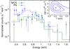 |
Fig. 3 PN (crosses) and MOS (diamonds) spectra and the best-fit model (blue dashed line for PN and green solid line for MOS). The inset (upper right corner) shows the 1-, 2-, and 3-sigma confidence contours for the temperature and emission measure. |
Figure 3 shows the PN and MOS spectra along with our best-fit spectral model, which describes the data well. The data quality remains insufficient to distinguish other spectral features such as emission lines. Our best-fit model yields a coronal temperature of  keV, corresponding to
  K, and an emission measure of
  cm-3 assuming a distance of 80 pc.
To estimate confidence intervals, we used XSPEC’s steppar command, which computes a grid of models for various temperatures and emission measures. The one, two, and three sigma confidence levels are offset from the minimum value of the C-statistic by 2.3, 4.61, and 9.21 (Press et al. 2002; Cash 1979). The corresponding contours are shown in Fig. 3 (upper-right corner). Based on the models, we determined the source flux and errors using the XSPEC flux and error commands. The resulting soft, unabsorbed X-ray flux amounts to  ergscm-2s-1 in the 0.2 − 2.0 keV band. Combining this with a distance of 80 ± 20 pc, we arrive at a luminosity of
  ergss-1. We note that the precise depth of the interstellar absorption column remains irrelevant for our results. In particular, we checked the fits made without absorption and with an absorption column deeper by an order of magnitude. While the best-fit temperature changes by no more 2%, we obtain a 13% increase in the emission measure for the deeper absorption column. For the probed column depths, the resulting best-fit estimates are still contained within the current 1-σ confidence intervals. While the unknown absorption column hardly affects the derived temperature, the uncertainty in the emission measure may be larger by about 50% taking the unknown absorption into account.
3. Discussion
Based on the effective temperature and the stellar radius, we derived a bolometric luminosity of Lbol = (6.4 ± 0.7) × 1032 ergs-1 for WASP-43, which is consistent with a K7V main-sequence star (de Jager & Nieuwenhuijzen 1987). For the ratio of X-ray and bolometric luminosity, LX/Lbol, we found a value of (1.0 ± 0.54) × 10-5 and, hence, log (LX/Lbol) = −4.98 ± 0.23. This is about one order of magnitude higher than the value of ≈1.2 × 10⁻⁶ observed for the Sun at maximum activity (max(LX, ⊙) ≈ 4.7 × 1027 ergs-1 in the ROSAT band, Peres et al. 2000) and is therefore compatible with the idea that WASP-43 is a younger and faster rotating star than the Sun.
3.1. X-ray luminosity versus stellar rotation period
In late-type stars the X-ray luminosity strongly correlates with rotation – and, therefore, age – as long as the saturation regime is not reached (Pizzolato et al. 2003). In their study, Pizzolato et al. (2003) analyzed the relation between X-ray emission and rotation in 259 low-mass stars. Field stars with a rotation period of ≈15.6 d show log (LX/Lbol) ratios between about − 6 and − 4.7. Among these, WASP-43 would, therefore, qualify as an active, but certainly not an outstanding, star. In fact, the log (LX/Lbol) ratio seems also to be compatible with the numbers Pizzolato et al. (2003) reported for the slower rotators among their sample of cluster stars with an age between about 40 and 600 Ma, which all rotate with periods ≲12 d, however.
We note that if the rotation period of WASP-43 were 7.8 d – another strong peak in the periodogram computed by Hellier et al. (2011), which they attributed to the first harmonic of the true period –, the relation given by Pizzolato et al. (2003) would suggest an X-ray luminosity of ≳5 × 1028 ergs-1. As this is inconsistent with our findings, our results support the interpretation given by Hellier et al. (2011).
Schmitt & Liefke (2004) analyzed the X-ray emission from low-mass stars in the solar neighborhood. The authors reported X-ray detections for all but two K-stars up to a distance of 12 pc. Comparing surface X-ray flux of WASP-43, Fs, of log (Fs [erg cm-2 s-1 ] ) = 5.4 ± 0.23 with the distribution found by Schmitt & Liefke (2004; their Fig. 8), we found that 70% of the K-stars in the solar neighborhood are less active than WASP-43 in terms of X-ray emission. Again, WASP-43 qualifies as active, but not unusual.
To determine whether the X-ray luminosity of WASP-43 is reasonable for a young (≈400 Ma) K-star, we compared it with the luminosity distribution in the similarly aged Hyades cluster (625 ± 50 Ma, Perryman et al. 1998). The Hyades have extensively been studied in X-rays using ROSAT data (Stern et al. 1995). Among single K-stars, Stern et al. (1995) detected about 25% with an X-ray luminosity higher than their detection limit of 9 × 1027 erg s-1. Although the distribution has not been probed to lower luminosities, we conclude that WASP-43 would most likely be found among the more X-ray luminous half of single K-stars in the Hyades. Although WASP-43’s gyrochronological age is compatible with its level of X-ray emission, we note that both are essentially determined by the rotation rate and are, consequently, not independent.
3.2. Planetary structure
Fortney et al. (2007) presented age-dependent model calculations of planetary structure considering various core masses and levels of insolation. Gillon et al. (2012) stated that the high mean density of WASP-43b – about 1.7 times the mean density of Jupiter according to our calculations – indicates a large core and an “old” age.
Our findings corroborate the age estimate of ≈400 Ma for WASP-43 derived by Hellier et al. (2011), and we assume that the star and its planet are coeval. In their calculations, Fortney et al. (2007) applied solar irradiation. Because WASP-43 is about six times fainter than the Sun in terms of bolometric luminosity, we applied an effective semi-major axis of 0.015 AU AU to compare their models with WASP-43b. In particular, we compared the mass and radius of WASP-43b to model calculations for giant planets with an age of 300 Ma (their Table 2). Extrapolating their result, we found that the mass and radius of WASP-43b are compatible with a core mass of ≈130 M⊕. This implies that the mass fraction of heavy elements in WASP-43b amounts to roughly 20%. Based on the same models, our solar system Jupiter reaches a core mass of 25 M⊕ or, equivalently, a heavy-element mass-fraction of 8%. We emphasize that neither the heavy element content of Jupiter nor the structure of its core are well known. For instance, Guillot et al. (1997) derived a value between 11 and 45 M⊕ for the total heavy-element content of Jupiter and argued that this mass is not necessarily concentrated in a core. Cautioning against this uncertainty, we conclude that the application of the Fortney et al. (2007) models to Jupiter and WASP-43b indicates that the fraction of heavy elements in WASP-43b is about twice as large as in Jupiter.
3.3. Implications for planetary mass-loss
High-energy X-ray and EUV radiation is efficiently absorbed in the upper planetary atmosphere, where it gives rise to activity-induced heating. The additional energy is thought to drive a planetary wind, which ultimately results in mass loss. While we were able to measure the X-ray component of the stellar high-energy emission, the EUV flux component can only be estimated because of interstellar absorption. Applying the relation between X-ray and EUV flux given by Sanz-Forcada et al. (2011), we estimated the stellar EUV luminosity, obtaining log (LEUV [ erg s-1 ] ) = 28.7 ± 0.5 or, equivalently, 2 × 1028 < LEUV < 2 × 1029 erg s-1. The EUV luminosity is, therefore, expected to be at least similar to the X-ray luminosity and probably higher by a factor of 3 − 30.
The X-ray flux at the orbital distance of the planet amounts to FX,orb = (10.2 ± 5.4) × 103 erg cm-2 s-1, which exceeds the X-ray flux experienced by Earth by about four orders of magnitude, but remains one order of magnitude below the level of X-ray irradiation the hot Jupiter CoRoT-2b is exposed to (Schröter et al. 2011). The total energy currently received by the planet in form of soft X-rays amounts to (1.75 ± 0.9) × 1024 erg s-1. Considering the wide range of estimates for the EUV irradiation at the planetary orbit (3 × 10⁴ − 3 × 10⁵ erg cm-2 s-1), we proceeded by adopting a combined X-ray and EUV flux, FXUV, of 105 erg cm-2 s-1 at the orbital distance. However, this remains an order of magnitude estimate because of the uncertainties in the EUV flux. We used Eq. (1) from Sanz-Forcada et al. (2011)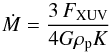 (6)to derive the mass-loss rate. Here, G is the gravitational constant, ρp is the mean density of the planet, and K accounts for enhanced losses due to tidal interactions. Energy-limited mass-loss with maximum heating efficiency as described by Eq. (6) provides the highest possible mass-loss rate in an unextended atmosphere, and the resulting values are therefore to be interpreted as upper limits. Using a factor of K = 0.53 (Erkaev et al. 2007), we estimate a mass-loss rate of Ṁ ≈ 1012 gs-1 or, equivalently, 0.017 MJGa-1 for WASP-43b. Multiplying this rate by the stellar age of ≈400 Ma yields 2 M⊕ for the total amount of mass lost by the planet.
The mass-loss calculations carried out above must be treated with caution considering the substantial uncertainties in the EUV flux and the limitations of the planetary mass-loss theory applied here. Furthermore, the stellar XUV flux was probably higher in the past. According to Pizzolato et al. (2003), the highest activity level of WASP-43, reached for a rotation period of about ≲3 − 4 d, yields a log (LX/Lbol) ratio of − 3.9. This would correspond to an X-ray luminosity of 8 × 1028 ergs-1 and, using the Sanz-Forcada et al. (2011) relation, an XUV flux of 8 × 10⁵ ergcm-2s-1 at the planetary orbit. Assuming this flux, we estimate an upper limit of 16 M⊕ for the time-integrated planetary mass-loss. If the planet has been substantially larger in the past, this would favor even higher loss rates (e.g., Valencia et al. 2010). We note, however, that the planet may not always have resided in such close proximity to the star. Furthermore, XUV radiation may become a less efficient driver of mass-loss for high irradiation levels (Murray-Clay et al. 2009).
If these estimates are anywhere close to reality, WASP-43b has likely neither lost more then about 16 M⊕ or 2.5% of its current mass so far, nor is it expected to loose much more mass in the future because stellar activity, and, therefore, high-energy emission, will fade away (e.g., Skumanich 1972). We note that energy-limited atmospheric escape, as considered above, may not be the only channel through which planetary mass-loss occurs. Khodachenko et al. (2007) found that the interaction between coronal mass ejections and the planetary atmosphere can lead to substantial mass-loss rates with a strong dependence on the planetary magnetic field, however.
If the mass-loss rate has been higher, we speculate that the removal of light elements from the planetary envelope may have contributed to the high observed mean density of the planet. Assuming that WASP-43b initially had a Jovian heavy-element mass-fraction of 10% and that only H and He are lost through atmospheric escape, would require huge mass-loss rates on the order of ≈3 × 10¹⁴ gs-1, however. We therefore argue that activity-induced mass-loss is unlikely to have a substantial impact on the evolution of the planet and that it has formed in an environment different from that of Jupiter.
4. Conclusion
We detected X-ray emission from WASP-43, which is currently the second-least-massive star known to host a hot Jovian planet. Although the star appears to be among the more active stars compared with K-stars in the solar neighborhood and in the Hyades, it is not exceptionally active. We conclude that its X-ray properties are compatible with the presence of strong Ca II H and K emission line-cores, the rotation period of 15.6 d, and the resulting gyrochronological age estimate of  Ma reported by Hellier et al. (2011). These authors noted that their stellar age estimate might be affected by tidal star-planet interactions spinning-up the star. Because activity is mainly driven by rotation, our results do neither require nor rule out this scenario.
The planet shows a relatively high mean density, which does not seem to be associated with an overabundance of metals in the entire system because the host star shows basically solar iron abundances (Table 1). According to the model calculations presented by Fortney et al. (2007), WASP-43b has a core-mass of roughly 130 M⊕, which is larger then the summed core mass of all solar system planets.
Orbiting an active star in one of the closest known orbits, the planet is immersed in an intense high-energy radiation field, which does not reach the magnitude of the most extreme example CoRoT-2b, however (Schröter et al. 2011). In view of our mass-loss estimates, it is unlikely that the planetary wind, thought to be driven by the stellar high-energy irradiation, has led to more than a 2.5% decrease in mass – neither is the planet expected to loose much more mass in the future. Although we speculate that activity-induced mass-loss could, indeed, have contributed to the high mean density of the planet, we regard it more likely that the explanation will be found in the formation process and the environment in which the planet formed. However, these may still have been affected by high-energy irradiation and, thus, stellar activity. The WASP-43 system may represent another opportunity to actually measure the activity-induced mass-loss through X-ray and UV absorption measurements, as has been demonstrated for HD 189733 and HD 209458 (Poppenhaeger et al. 2013; Vidal-Madjar et al. 2003; Lecavelier Des Etangs et al. 2010).
Checked with http://www.exoplanets.org (Wright et al. 2011).
Acknowledgments
P.C.S. acknowledges DLR support (50OR1307). M.S. acknowledges support by the DFG Graduiertenkolleg 1351 “Extrasolar Planets and their Host Stars”.
References
- Arnaud, K. A. 1996, in Astronomical Data Analysis Software and Systems V, eds. G. H. Jacoby, & J. Barnes, ASP Conf. Ser., 101, 17 [Google Scholar]
- Cash, W. 1979, ApJ, 228, 939 [NASA ADS] [CrossRef] [Google Scholar]
- de Jager, C., & Nieuwenhuijzen, H. 1987, A&A, 177, 217 [NASA ADS] [Google Scholar]
- Erkaev, N. V., Kulikov, Y. N., Lammer, H., et al. 2007, A&A, 472, 329 [NASA ADS] [CrossRef] [EDP Sciences] [Google Scholar]
- Fortney, J. J., Marley, M. S., & Barnes, J. W. 2007, ApJ, 659, 1661 [NASA ADS] [CrossRef] [Google Scholar]
- Foster, A. R., Ji, L., Smith, R. K., & Brickhouse, N. S. 2012, ApJ, 756, 128 [NASA ADS] [CrossRef] [Google Scholar]
- Gillon, M., Triaud, A. H. M. J., Fortney, J. J., et al. 2012, A&A, 542, A4 [NASA ADS] [CrossRef] [EDP Sciences] [Google Scholar]
- Grevesse, N., & Sauval, A. J. 1998, Space Sci. Rev., 85, 161 [NASA ADS] [CrossRef] [Google Scholar]
- Guillot, T., Gautier, D., & Hubbard, W. B. 1997, Icarus, 130, 534 [NASA ADS] [CrossRef] [Google Scholar]
- Hellier, C., Anderson, D. R., Collier Cameron, A., et al. 2011, A&A, 535, L7 [NASA ADS] [CrossRef] [EDP Sciences] [Google Scholar]
- Jackson, B., Miller, N., Barnes, R., et al. 2010, MNRAS, 407, 910 [NASA ADS] [CrossRef] [Google Scholar]
- Johnson, J. A., Gazak, J. Z., Apps, K., et al. 2012, AJ, 143, 111 [NASA ADS] [CrossRef] [Google Scholar]
- Khodachenko, M. L., Lammer, H., Lichtenegger, H. I. M., et al. 2007, Planet. Space Sci., 55, 631 [NASA ADS] [CrossRef] [Google Scholar]
- Lammer, H., Selsis, F., Ribas, I., et al. 2003, ApJ, 598, L121 [NASA ADS] [CrossRef] [Google Scholar]
- Laughlin, G., Bodenheimer, P., & Adams, F. C. 2004, ApJ, 612, L73 [NASA ADS] [CrossRef] [Google Scholar]
- Lecavelier Des Etangs, A., Ehrenreich, D., Vidal-Madjar, A., et al. 2010, A&A, 514, A72 [NASA ADS] [CrossRef] [EDP Sciences] [Google Scholar]
- Murray-Clay, R. A., Chiang, E. I., & Murray, N. 2009, ApJ, 693, 23 [Google Scholar]
- Peres, G., Orlando, S., Reale, F., Rosner, R., & Hudson, H. 2000, ApJ, 528, 537 [NASA ADS] [CrossRef] [Google Scholar]
- Perryman, M. A. C., Brown, A. G. A., Lebreton, Y., et al. 1998, A&A, 331, 81 [NASA ADS] [Google Scholar]
- Pizzolato, N., Maggio, A., Micela, G., Sciortino, S., & Ventura, P. 2003, A&A, 397, 147 [NASA ADS] [CrossRef] [EDP Sciences] [Google Scholar]
- Poppenhaeger, K., Czesla, S., Schröter, S., et al. 2012, A&A, 541, A26 [NASA ADS] [CrossRef] [EDP Sciences] [Google Scholar]
- Poppenhaeger, K., Schmitt, J. H. M. M., & Wolk, S. J. 2013, ApJ, 773, 62 [NASA ADS] [CrossRef] [Google Scholar]
- Press, W. H., Teukolsky, S. A., Vetterling, W. T., & Flannery, B. P. 2002, Numerical recipes in C++: the art of scientific computing (CUP) [Google Scholar]
- Sanz-Forcada, J., Micela, G., Ribas, I., et al. 2011, A&A, 532, A6 [NASA ADS] [CrossRef] [EDP Sciences] [Google Scholar]
- Schmitt, J. H. M. M., & Liefke, C. 2004, A&A, 417, 651 [NASA ADS] [CrossRef] [EDP Sciences] [Google Scholar]
- Schröter, S., Czesla, S., Wolter, U., et al. 2011, A&A, 532, A3 [NASA ADS] [CrossRef] [EDP Sciences] [Google Scholar]
- Skumanich, A. 1972, ApJ, 171, 565 [NASA ADS] [CrossRef] [Google Scholar]
- Stern, R. A., Schmitt, J. H. M. M., & Kahabka, P. T. 1995, ApJ, 448, 683 [Google Scholar]
- Valencia, D., Ikoma, M., Guillot, T., & Nettelmann, N. 2010, A&A, 516, A20 [NASA ADS] [CrossRef] [EDP Sciences] [Google Scholar]
- Vidal-Madjar, A., Lecavelier des Etangs, A., Désert, J.-M., et al. 2003, Nature, 422, 143 [NASA ADS] [CrossRef] [PubMed] [Google Scholar]
- Wang, W., van Boekel, R., Madhusudhan, N., et al. 2013, ApJ, 770, 70 [NASA ADS] [CrossRef] [Google Scholar]
- Wright, J. T., Fakhouri, O., Marcy, G. W., et al. 2011, PASP, 123, 412 [NASA ADS] [CrossRef] [Google Scholar]
All Tables
Source count-rate as a function of background filtering cut-offs in the 0.2 − 2.0 keV band.
All Figures
|
Fig. 1 High-energy PN light curve (10 − 12 keV, 100 s binning). The horizontal lines indicate the default (0.4 cts-1, dotted) and 2.5 times elevated (1 cts-1, dashed) cut-offs. The good-time intervals for the elevated cut-off are indicated by the shading. |
| In the text | |
|
Fig. 2 PN image of WASP-43 (0.2 − 2 keV band). The labeled black circle depicts the source region, the larger blue regions are used for background extraction. |
| In the text | |
|
Fig. 3 PN (crosses) and MOS (diamonds) spectra and the best-fit model (blue dashed line for PN and green solid line for MOS). The inset (upper right corner) shows the 1-, 2-, and 3-sigma confidence contours for the temperature and emission measure. |
| In the text | |
Current usage metrics show cumulative count of Article Views (full-text article views including HTML views, PDF and ePub downloads, according to the available data) and Abstracts Views on Vision4Press platform.
Data correspond to usage on the plateform after 2015. The current usage metrics is available 48-96 hours after online publication and is updated daily on week days.
Initial download of the metrics may take a while.