| Issue |
A&A
Volume 560, December 2013
|
|
|---|---|---|
| Article Number | A102 | |
| Number of page(s) | 10 | |
| Section | Interstellar and circumstellar matter | |
| DOI | https://doi.org/10.1051/0004-6361/201322220 | |
| Published online | 12 December 2013 | |
Spatially resolved physical and chemical properties of the planetary nebula NGC 3242⋆
1 Departamento de Física e Química, Universidade Federal de Itajubá, Itajubá MG, Brazil
e-mail: hmonteiro@unifei.edu.br
2 Observatório do Valongo, Universidade Federal do Rio de Janeiro, Ladeira Pedro Antonio 43, 20080-090 Rio de Janeiro, Brazil
3 Argelander-Institut für Astronomie, University of Bonn, Auf dem Hügel 71, 53121 Bonn, Germany
4 Instituto de Astrofísica de Canarias, 38200 La Laguna, Tenerife, Spain
5 Departamento de Astrofísica, Universidad de La Laguna, 38206 La Laguna, Tenerife, Spain
Received: 5 July 2013
Accepted: 17 October 2013
Aims. Optical integral-field spectroscopy was used to investigate the planetary nebula NGC 3242. We analysed the main morphological components of this source, including its knots, but not the halo. In addition to revealing the properties of the physical and chemical nature of this nebula, we also provide reliable spatially resolved constraints that can be used for future photoionisation modelling of the nebula. The latter is ultimately necessary to obtain a fully self-consistent 3D picture of the physical and chemical properties of the object.
Methods. The observations were obtained with the VIMOS instrument attached to VLT-UT3. Maps and values for specific morphological zones for the detected emission-lines were obtained and analysed with routines developed by the authors to derive physical and chemical conditions of the ionised gas in a 2D fashion.
Results. We obtained spatially resolved maps and mean values of the electron densities, temperatures, and chemical abundances for specific morphological structures in NGC 3242. These results show the pixel-to-pixel variations of the the small- and large-scale structures of the source. These diagnostic maps provide information free from the biases introduced by traditional single long-slit observations.
Conclusions. In general, our results are consistent with a uniform abundance distribution for the object, whether we look at abundance maps or integrated fluxes from specified morphological structures. The results indicate that special care should be taken with the calibration of the data and that only data with extremely good signal-to-noise ratio and spectral coverage should be used to ensure the detection of possible spatial variations.
Key words: planetary nebulae: general / planetary nebulae: individual: NGC 3242 / ISM: abundances
© ESO, 2013
1. Introduction
Planetary nebulae (PNe) are end products of the evolution of stars with masses from approximately 0.8 to 8 M⊙ and as such have great importance in many fields in astrophysics, from basic atomic processes in solar-like stars to distant galaxies. Although the general picture of planetary nebulae formation is well understood (Kwok 2008), many questions remain unsolved, such as the mechanism by which the material ejected by the star finally forms the many observed morphologies (Balick & Frank 2002).
NGC 3242 is a multiple-shell PN within a bright 28′′ × 20′′ inner elliptical shell, which also contains a pair of ansae (or, small-scale low-ionisation structure, LIS; Gonçalves et al. 2001). The inner shell is surrounded by a fainter 46′′ × 40′′ moderately elliptical envelope (see, for instance, Ruíz et al. 2011). These two shells are further more enclosed by concentric rings and a giant broken halo revealed by deep images (Corradi et al. 2004; Monreal-Ibero et al. 2005).
The bright central star (V = 12.43) of the nebula has been studied by several authors. Different methods for evaluating its effective temperature (Teff) were applied, which thus culminates in a wide range of possible values. In a detailed discussion, Pottasch & Bernard-Salas (2008) showed that the hydrogen Zanstra temperature is 57 000 K, while the helium Zanstra temperature is 90 000 K. From stellar atmospheric models the Teff is found to be 75 000 K (Pauldrach et al. 2004), but temperatures as high as 94 000 K are found in the literature (Tinkler & Lamers 2002). After analysing this wide range of possibilities and taking into account the higher helium Zanstra temperature, Pottasch & Bernard-Salas (2008) assumed in their work a temperature of 80 000 K for the central star of NGC 3242, which leads to a luminosity of 730 L⊙, with a radius of 0.141 R⊙. Notice, however, that other authors have found higher values for the luminosity of this nebula. For example, the 3200 L⊙ found by Pauldrach et al. (2004). The mass-loss rate of the central star is estimated to be ≤2 × 10⁻⁸ M⊙/yr (Kudritzki et al. 1997) and the post-asymptotic giant branch mass is believed to lie between 0.53 M⊙ and 0.56 M⊙. The latter value corresponds to an MS star of 1.2 ± 0.2 M⊙ (Galli et al. 1997; Stanghellini & Pasquali 1995; Pauldrach et al. 2004).
For the nebula in the radio wavelength – its optical properties are discussed in details below –, the H91α recombination line and the 3.5 cm continuum observations (Rodríguez et al. 2010) give nebular temperatures (10 100 ± 700 K) consistent, within 10%, with that obtained from optical lines and the Balmer discontinuity (Liu & Danziger 1993; Krabbe & Copetti 2006). Moreover, that the LTE continuum and the line H91α temperatures agree very well is in proof itself that a significant continuum contamination by dust emission is absent from this nebula. Still following Rodríguez et al. (2010), the radio continuum measurements can be interpreted as being completely due to free-free emission, without the 30 GHz excess previously suggested by Casassus et al. (2007).
The observations of Ruíz et al. (2011), taken with the XMM-Newton, have shown that the X-ray luminosity of NGC 3242 is ~2 × 1030 erg s-1 for an adopted distance of 0.55 kpc (Terzian 1997; Mellema 2004). Following the same authors, the temperature of the hot-bubble region in which the X-rays are produced is ~2.35 × 10⁶ K. These figures agree with the ad hoc predictions of the shock-heated stellar wind models confined by heat conduction.
Few works address the question of the spatial variation of the nebular properties, and if they do, they use traditional long-slit data. One example is the study of Perinotto & Corradi (1998) about 20 PNe (mostly Type I), showing that PNe are in general chemically homogeneous. Balick et al. (1994) reported that a few objects (specifically, NGC 6543, 6826, and 7009) showed significant abundance variations from one component to another, but subsequent 3D photoionisation modelling did not confirm it (Gonçalves et al. 2006). Although NGC 3242 is a well-known PN, with about 350 references from 1990 to date, and even though different diagnostics were clearly determined, only few works investigated its characteristics using some kind of spatially resolved data, from a range of wavelengths. Monreal-Ibero et al. (2005), the only work apart from ours that used IFU data for this object, succeeded in determining some properties of the halo, but did not perform a detailed analysis of the physical and chemical properties.
Our aim here is to derive the ionic and total element abundances for NGC 3242 in a spatially resolved way from VLT VIMOS IFU data. We aim to address the question of the chemical abundance variation within the PN. Our motivation is that, in principle, material at different positions within a PN (or different PN components) may be the result of distinct mass-loss episodes of the progenitor star and therefore may trace the chemical inhomogeneities (enrichment) in the original (not coeval) outflows.
In Sect. 2 we discuss the data and their reduction, while in Sect. 3 we show the results obtained from the emission maps. In Sect. 4 we present the results for specific morphological structures on which fluxes were integrated, and in Sect. 5 we conclude.
2. Data acquisition and reduction
The observations were obtained with the instrument VIMOS-IFU, attached to VLT-UT3. The instrument is composed of 6400 fibers and, has a changeable scale on the sky that was set to 0.67′′ per fiber, to obtain our data. The image is formed by a matrix of 80 × 80 fibers, which gave us a coverage of 54′′ × 54′′ on sky. We obtained observations in low-resolution mode, with a pixel scale of 5 Å pix-1 with a spectral coverage of 3290 Å, yielding a useable range from 3900 Å to 7000 Å, and in high-resolution mode with a pixel scale of 0.6 Å pix-1, yielding a spectral coverage of 2200 Å, from 5250 Å to 7450 Å. The reduction was performed with the VIMOS pipelines available at the instrument website1. A typical spectrum from the IFU data is shown in Fig. 1 where the data for spaxel (50,30) are displayed.
Owing to poor weather we were unable to observe a standard star. To overcome this limitation, we opted to flux-calibrate the data with respect to a long-slit spectrum of the object, obtained at a posterior date, and kindly provided by R. Costa, as described below.
Because we had a resolved emission map of the nebula for all detected emission lines, the procedure to perform flux calibration was essentially the comparison of pixels in the emission maps obtained from the IFU data with a given observed long-slit configuration. In an ideal situation, a given area extracted from the IFU-calibrated maps should give the same integrated flux values as an equivalent aperture or slit from a distinct observation. Clearly, atmospheric variations very likely have a significant impact on the final fluxes because of different seeing and extinction values. However, because we scaled the emission-line maps to match an integrated flux for a given long-slit area, at least the relative flux variations within the maps were preserved.
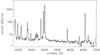 |
Fig. 1 Spectrum from the spaxel (50,30) showing typical features and quality of the data. |
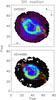 |
Fig. 2 Line-emission maps for [O iii] λ5007 (top) and Heiiλ4686 (bottom) showing the position of the long-slit observations used for the flux calibration of the data (red dotted lines). The orientation in the sky as well as the plate scale is also indicated in the top map. The contours overlaid in both figures are of the [N ii]6584 line-emission map. In the maps above the intensity scale is normalised to the maximum value for each emission line. |
In Fig. 1 we show the position of the long-slit used in the flux calibration of the data as well as emission-line map information that is discussed in detail below. It is clear from the figure that the slit position misses the bright parts of both knots of the nebula. It is also evident that the slit only captures the lowest intensity part of the He ii 4686 Å emission.
3. Results
In Fig. 3 we show the emission-line maps for the stronguest lines we detected, which were used as diagnostic of the electron densities, temperatures, and chemical abundance. The maps show a clear sensitivity variation from one lens array to another (see, for example, the emission-line map of [S ii] in Fig. 3). Although these variations are sometimes not clear in a given emission-line map, they become more evident in some diagnostic ratio maps, as discussed below. There are also dead fibers in some of the quadrants. These problems are documented in the instrument pages (VLT-IFU) pages and we refer to them for further details. In short, we were able to correct for some of the artifacts generated by these problems, but not all could be removed.
Because we not deal with integrated fluxes, the typical signal-to-noise ratio (S/N) in a volumetric pixel (voxel) of the data cube can be significantly lower in comparison. In practice, the trade-off of spatial resolution is lower S/N in a given pixel of the observed map. For individual emission-line maps the limited S/N is no great problem, but it results in significant noise when spatially detailed diagnostic ratio maps are computed. To improve the quality of the final maps we applied a fast Fourier filter to remove some of the noise, especially in the low S/N regions. Areas with a S/N below 5 were completely removed and their signal was set to 0.
3.1. Extinction coefficient, densities, and temperatures
Total line fluxes relative to Hβ obtained from the emission-line maps and compared with the total fluxes of Tsamis et al. (2003; T03).
To work with the emission line maps presented in Fig. 3 and derive the nebular properties (internal extinction, electron densities, and temperatures as well as ionic and total chemical abundances), we used the program 2d_neb. This program is based on the well established IRAF nebular package, and was developed to enable the use of the spectroscopic maps to easily obtain the astrophysical quantities of ionised nebulae also in the form of maps. The 2d_neb package uses the traditional line-ratio diagnostics and the atomic data from IRAF to derive Ne and Te. The process is based on the iraf.nebular.temden task and consists of solving the equation of statistical equilibrium. The ionic abundance calculation follows the iraf.nebular.ionic task, complemented by the atomic data given by Benjamin et al. (1999). The total chemical abundances maps are derived using the ionisation correction factors (ICFs) given by Kingsburgh & Barlow (1994) and Liu et al. (2000) (see Leal-Ferreira et al. 2011, for more details on the 2d_neb code).
The first step in this analysis was the determination of the extinction coefficient c(Hβ) using the Balmer decrement. Because the Hα line was saturated in a number of pixels and the Hβ, Hγ, and Hδ line-ratios only provided noisy ratio maps, we computed an average c(Hβ) value from the Balmer line fluxes integrated over the whole nebula. We adopted the extinction curve given by Cardelli et al. (1989), updated by O’Donnell (1994), with Rν = 3.1. We derived c(Hβ) = 0.25 (Table 1), which is consistent with values from the literature, which are around 0.2 (Balick et al. 1993; Henry et al. 2000; Tsamis et al. 2003; Pottasch & Bernard-Salas 2008). We adopted this value to correct all the VIMOS-IFU emission-line maps we observed for extinction.
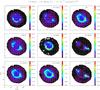 |
Fig. 3 Emission-line maps for the most important lines observed with VIMOS-IFU. From top to bottom and left to right, they are [Ar iv] 4711 Å; [Cl iii] 5537 Å; Hβ; He i 5876 Å; He ii 4686 Å; [N ii] 6584 Å; [O iii] 5007 Å; [O iii] 4363 Å; and [S ii] 6731 Å. The orientation in the sky and the plate scale is the same as in Fig. 1. The intensity scale is normalised to the maximum value for each emission line. |
The extinction-corrected emission-line maps were used to derive the spatial distribution of the electron density (Ne) and temperature (Te) of the nebula. By assuming a constant Te throughout the nebula we obtained a first estimate for the Ne maps based on the [S ii], [Cl iii] and [Ar iv] lines. The estimated maps were used in an iterative procedure to obtain the final Ne and Te maps. The results for the density are shown in Fig. 4. The mean values of the electron densities, weighted by the most intense line map used in the ratio, were Ne[Ar iv] = 2640 cm-3, Ne[Cl iii] = 2380 cm-3, and Ne[S ii] = 3120 cm-3. Since most of the works in the literature reported values obtained from integrated fluxes, we present these quantities and their associated errors in Table 2, together with results taken from the literature. Considering that errors are not quoted in all previous works shown in Table 2, our means agree reasonably well with the other density estimations.
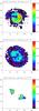 |
Fig. 4 Diagnostic ratio maps for the electron density derived from the [Ar iv], [Cl iii] and [S ii] emission-lines. The orientation in the sky as well as the plate scale are the same as in Fig. 2. |
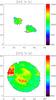 |
Fig. 5 Diagnostic ratio maps for the electron temperature derived from the [N ii] and [O iii] emission maps. The orientation in the sky as well as the plate scale are the same as in Fig. 2. |
Densities and temperatures derived from typical diagnostic line ratios, from our maps (mean values) compared to with some selected previous works.
To derive the electron temperature maps, we used the Ne maps previously described (Fig. 4) as input parameters. To obtain the final temperature maps the calculations were performed pixel by pixel, each with its respective density value. As usual, the similarity of the ionisation potential was the criterion for adopting Te[N ii] or Te[O iii], and [S ii] or [Ar iv] densities. Our temperature maps are presented in Fig. 5 and correspond to mean values of 11 670 K and 12 900 K for Te[N ii] and Te[O iii], respectively. The figures show that the temperature distribution is very constant in both maps apart from an increase in the rim region seen in the Te[O iii] map. Within the rim, however, the temperature shows little fluctuation. The temperatures found in our maps are consistent with values determined by Monreal-Ibero et al. (2005) within their quoted uncertainties.
3.2. Ionic and total chemical abundances
The Ne and Te maps were used as input to determine ionic abundances. They are accounted for such that low- (Te[N ii], Ne[S ii]) and medium- (Te[O iii], Ne[Ar iv], Ne[Cl iii]) excitation electron temperatures and densities are, correspondingly, adopted for the low-([O i], [S ii] and [N ii]) and intermediate-ionisation ions ([O iii], [Cl iii], [S iii] and [Ar iv]). The ionic abundance obtained in this work from the mean fluxes of Table 2 values are show in Table 3, where those from the literature are also given for comparison.
To obtain the total chemical abundance maps we followed the prescriptions by Kingsburgh & Barlow (1994) when only optical data is available. These authors provided the ICFs that account for the ionic maps we cannot calculate from our data. For oxygen, a key ionic map, O+/H+, is missing, because the VIMOS configuration does not include either the [O ii] 3727 Å or the 7325 Å emission lines. Therefore, we generated ionic abundance maps from values found in the literature (2.54 × 10⁻⁶ and 4.16 × 10⁻⁶ for O+/H+ based on 3727 Å and 7325 Å, respectively, T03) and assumed that these abundances are uniform throughout the map. We then calculated the average of these two uniform maps (=3.35 × 10⁻⁶), generating a final O+/H+ that we used to obtain the ICFs. This was necessary because without this ionic map, the total abundance of oxygen (O/H) cannot be calculated, and as a consequence,the entire ICF would be missing (see Kingsburgh & Barlow 1994, Appendix A).
Maps showing the total abundances of oxygen, nitrogen, sulphur, chlorine, and helium are shown in Fig. 6. By examining Fig. 6 we see no significant abundance variation of O, N, S or Cl (based on uncertainty estimates obtained in Sect. 4). It is also worth noting that for some elements only one ionic fraction is available. In these cases, the total abundances were determined only for the regions for which the corresponding emission-line is strong. The extreme example of this effect is observed for N+/H+. In Fig. 6 the strong LISs are the only structures for which we were able to derive the N/H.
Ionic and total abundances obtained from integrated line fluxes compared with those obtained in the literature.
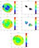 |
Fig. 6 Total abundance maps. The orientation in the sky as well as the plate scale are the same as in Fig. 2. |
Several authors have obtained ionic and total abundances of He and the most abundant heavy elements of NGC 3242, from long-slit spectra. Three of these abundances results are shown in Table 3 and are compared with our own calculated values, estimated from the total line fluxes. We point out that the wavelength coverage as well as the region covered by the slit/aperture vary in the literature. Krabbe & Copetti (2006) data covering the wavelength range from 3100 Å to 6900 Å, is closer to ours not only in terms of spectral coverage, but also in terms of the elemental abundances and ICFs derived although they use a single slit. Similar to our studie, their study was based on optical spectra alone. At the other extreme of reported values are those of Pottasch & Bernard-Salas (2008), who used the Spitzer Space Telescope and the Infrared Space Observatory for the near-IR wavelengths and the International Ultraviolet Explorer (IUE) as well as ground-based optical spectra, all of which have distinct apertures and slit sizes. It is worth noting that they needed no ICFs in their analysis, therefore their elemental abundances should be the best. The comparison shows that the Pottasch & Bernard-Salas (2008) results differ from ours by more than the other two sets of results. But on the whole, the difference in the abundances obtained in all the four papers is always small. The exception is the N abundance, an element for which the optical abundance is well-known to be poorly determined. The only way of improving the N/H abundances is by adding the UV spectrum to the optical and/or optical- plus- near-IR spectrum. Tsamis et al. (2003) scanned the slit across the nebula in the optical spectrum acquisition and added to the analysis IUE data. It is straightforward to see from Table 3 that their results are similar to ours, again with the exception of the nitrogen abundance.
Though within the range of expected values, the He/H abundance variations in the map are significant. To investigate this in more detail, we compared our mean He/H with the other values for the entire nebula in the literature (see Table 3). Inspecting the table, we see that our He/H, agrees with the other values reported in the literature , which indicates that our results are good at least on average.
Although they agree, within the errors, the total line fluxes and the differences between our values and those obtained by T03 may indicate that the current precision and accuracy obtained with the typical observing techniques may not be adequate for the investigation of spatial variation of chemical abundance.
4. Zone analysis: summing up the emission per region
As discussed above, a study of spatial abundance variations using the maps obtained, that are displayed in Fig. 6 is made difficult by the limited S/N in individual pixels. However, IFU data have the advantage that the signal can be integrated over given sets of pixels, for instance covering specific morphological components of the nebula. Given the symmetry of the object, we used isophotal contours to delineate the boundaries of nebular regions of particular interests. Specifically, we defined seven distinct zones that separate all of the major morphological features seen in the emission line maps. The zones and their boundaries are shown in the schematic Fig. 7. The largest and faintest zone is refered to as the shell. The second zone, commonly refered to as the rim, is the brightest and densest structure of the nebula.
The other zones were chosen to attend to the region of the bright knots (LISs) seen in images. Here we opted to divide the knot into two main parts in an attempt to isolate the knot from the other structures as much as possible. These two regions, defined for the two visible knots, are composed of the knots themselves and a tail that morphologically seems to lag behind the actual knots. In this way, the knots in principle contain the lowest possible contamination from the other zones and the tail also does not contain most of the emission of the knots. The tail zones overlap with the rim to some extent. The tails are are better visible in Fig. 8, where we show the zone contours overlaid on the emission maps of Hβ and [N ii]6584 Å. The tail and knot zones are defined such that the south knot is connected to zones tail a and knot a and the north knot with zones tail b and knot b. We also defined a final zone knot c connected to a structure that is very bright, in most emission-lines, and is situated at the bottom of tail a and on top of the rim.
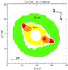 |
Fig. 7 Zone scheme definitions for NGC 3242. The orientation in the sky as well as the plate scale are the same as in Fig. 2. |
For each of these zones, we sumed up the fluxes and performed the same analysis as in the previous section. In Table 4 we present the total extinction-corrected fluxes, densities, temperatures, ionic abundances, and total abundances for each zone.
Physical parameters, ionic and total abundances, and ICFs obtained for each zone defined from isophotal contours.
Some of the previous works on NGC 3242 discussed above, which have data for the entire nebula (c(Hβ), Te, Ne and abundances), also reported spatially resolved estimates of physical properties for the rim, shell and for the knots. The most recent of these works is that of Ruíz et al. (2011) who pesented temperatures of 10 000 ≤ Te(K) ≤ 14 700 (8070 ≤ Te(K) ≤ 10 400) for the rim (shell). Although formal errors are not quoted, the general picture from the comparison of our results to this one is that their electron temperatures are systematically lower than ours. The discrepancy for the temperature is 1200 K and 2000 K when derived from the [N ii] and [O iii] ratios, respectively. We note that these differences are smaller than the dispersion in temperature due to the different emission-line ratios, which means that they are probably constrained within the errors. These authors derived, for the rim and shell, values for the electron densities that vary from 2200 to 2250 cm-3 and 340 to 400 cm-3, respectively. The two density diagnostics they used were [S ii] and [Ar iv], while we used [Cl iii] as well. In general, despite the different observational data and zone definitions, the results agree within the possible uncertainties which, for faint lines such as the [S ii], can reach 50%. The main differences are in the densities obtained from the [S ii] lines for the shell, but in this case our values should be taken with care, because of very low S/N for the line in this particular zone. The effect can be clearly seen in the [S ii] density map shown in Fig. 4. In the areas with a good S/N for the line the density values agree with those of the other authors.
Another comparison can be made with the long-slit data reported Balick et al. (1993). In that work, authors constructed a spatially resolved study of NGC 3242 and specifically discussed theknot. They derived [N ii] and [O iii] electron temperatures, and [S ii] and [Cl iii] densities for the four components of the nebula for which we derived the nebular properties shown in Table 4. Their Fig. 4 shows profiles of these quantities evaluated along the long-slit (PA = −30°). According to this figure, Te[O iii] (Te[N ii]) of bothknots are 10 000 to 11 000 K (~9000 K). These figures agree well with our results, especially for Te[N ii]. The trend of higher Te[O iii] than Te[N ii] is found in both works as well. Balick et al. (1993) found Te[O iii] = 11 000 K at the rim and shell and quoted that their uncertainty is of about 10%, which makes their results similar to ours apart from a higher Te[N ii] at the rim. However, this particular value should be taken with care because the highly localised emission from the [N ii] lines. They interpreted their results as indicating constant electron temperatures throughout the nebula. When densities are the focus, the values we found for the rim and shell are about half of those reported in Balick et al. (1993) for the two emission-line diagnostics in common. Despite the discrepancy, the values are within the large uncertainty mentioned above. The larger discrepancy is perhaps forknot b where we find a density of 3450 cm-3, which is similar to the rim density, again in contrast to the trend that was found by Balick et al. (1993). For this particular knot, due to its proximity to the rim, it is likely that some contamination from the nearby emission is present.
Indeed, the density map in Fig. 3 shows that the inconsistency disappears in the more precise pixel-by-pixel analysis for regions with a good S/N. The results indicate that although summing pixels in pre-defined zones may improve the S/N, it does not deal completely with the contamination from nearby zones. It is very likely that theknot a values for physical and chemical composition are more representative of the knots, because this structure it is less contaminated by the emission from the bright rim zone, as indicated by the densities found.
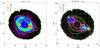 |
Fig. 8 Zone contours overlaid on observed emission-line maps of Hβ (left) and [N II] 6584 (right). The orientation in the sky as well as the plate scale are the same as in Fig. 2. |
The results of our analysis for the abundance variations within NGC 3242, are also shown in Table 4. We found no significant abundance contrast for He and O. The extreme case is N/H, whose shell abundance is more than twice that of the rim, and theknots are up to six times more abundant than the rim. The derived increase in abundance is apparent in both knots, indicating that the result is not influenced by nearby emission contamination. However, as discussed in Sect. 3.2, for this element the ICFs are typically very high (varying from 93 in the rim to 42 inknot a), which yields a very poor determination of the abundances because most of the nitrogen ionic fractions are beyond the optical spectrum (also see Gonçalves et al. 2006, 2012), indicating that the increases found are not reliable.
To obtain an estimate of the uncertainties involved in the abundance determinations we performed a Monte Carlo analysis using the total fluxes in Table 1. We calculated the abundances 5000 times, each time sampling a different flux value from a Gaussian distribution with the line flux as the mean and 5% and 10% total uncertainties (flux calibration+photon statistics) for strong and weak lines, respectively. The abundance 1σ uncertainties obtained are ≈10% for He, ≈15% for O, ≈35% for S, and ≈60% for N. Clearly, since we used the total fluxes, these error estimates are lower limits and are probably higher for regions of low S/N levels. When evaluating the results, however, it is important to point out that the adequacy of the ICFs used cannot be easily incorporated into the final uncertainties obtained, which essentially means that the actual errors can be even higher.
Finally, taking into account all the discussions and caveats pointed out above, and conservatively analysing Table 4, we find no abundance variations for the elements He and O in the rim,shell and knots of NGC 3242. We also infer that the abundance variation found for N (>6×), S (>2×), and Cl (>2×) are probably caused by the high ICFs, which prevents us from stating weather these results reflect the real conditions within the nebula.
5. Discussion and conclusions
We investigated the spatially resolved physical and chemical properties of the planetary nebula NGC 3242. The determination of the physical and chemical properties of the object obtained from our resolved IFU observations are in general consistent with those obtained in the literature from data with more limited spatial coverage. The comparison of the total fluxes obtained in this work with those of Tsamis et al. (2003) showed that our results agree well despite the indirect flux calibration we had to adopt, thus validating the procedure. The spatially resolved maps for the physical and chemical conditions show considerable structure. When considering the abundance maps, however, we did not infer significant abundance variations within the limits of the present data.
To investigate the abundance variations from another angle using the same data set, we also divided the nebula into zones for which we obtained total fluxes. The zones isolated the main morphological features of NGC 3242: the shell, the rim, and two knots. The results for the zone analysis corroborates other results from the literature and shoed no evidence for significant spatial variation of the chemical abundances of He and O, even in peculiar features such as the knots. In these features, we found an overabundance of N and S, but the uncertainties as well as the large ICFs used showed that the increase is not significant. Ideally, proper 3D modelling is needed to analyse the highly asymmetric structures as was performed in Gonçalves et al. (2006).
Several observational studies have investigated the question of possible spatial variations of the abundances in PNe using long-slit optical data. An example is the study of Perinotto & Corradi (1998), who analysed thirteen PNe with a bipolar morphology. These authors found that the He, O, and N abundances were constant throughout all the nebulae studied. The abundances of Ne, Ar, and S were also found to be constant within the errors, but their face values implied a systematic increase toward the outer regions of the nebulae. On the other hand, other authors (Balick et al. 1994; Guerrero et al. 1995) found element overabundance high factors (2 to 5) for a few PNe. Particularly, evidence was found for overabundance of nitrogen from studying the LISs of some PNe, compared ith the N/H of the main (rims, attached shells, halos) of the same PNe (Balick et al. 1994; Gonçalves et al. 2003). However, at least for NGC 7009 (Balick et al. 1994; Gonçalves et al. 2003), the supposed nitrogen overabundance in LISs was subsequently excluded by a detailed 3D photoionisation modelling of the nebula (Gonçalves et al. 2006). Therefore, nitrogen abundance variations are not reliable, when they are based on optical data alone, either using long-slit or IFU spectra with their correspondent ICFs. The main reason for this is that most of the emission lines from ions of N are not in the optical, but in the UV (see for example Alexander & Balick 1997; Gruenwald & Viegas 1998; Stasińska 2002; Henry et al. 2004; Gonçalves et al. 2006; Gonçalves 2013, among others). It is clear, therefore, that the current ionisation-correction methods for nitrogen are problematic. Moreover, for different reasons, but leading to a similar situation of low accuracy in the results, the variation of the sulphur abundances cannot be addressed by studies in the optical, or optical plus IR either (Henry et al. 2004; Shaw et al. 2010; Henry et al. 2012; Gonçalves 2013, and references therein). This is because the sulphur anomaly, which refers to the fact that PN sulphur abundances are systematically lower than those found in most other interstellar abundance probes for the same O abundance (or metallicity; Henry et al. 2004). Here again the ICFs seem to be the problem. The considerations above indicate that if we aim to address the possibility of chemical inhomogeneities in PNe, better ICFs are needed.
The link between different mass-loss episodes (of the PN and previous phases of the central star) and the resulting chemical inhomogeneities in the nebula have been investigated in the past, as can be seen in Balick et al. (1994); Hajian et al. (1997); Perinotto & Corradi (1998); Gonçalves et al. (2003, 2004, 2009); and Leal-Ferreira et al. (2011), among others. However, such a link has not been found yet. In the particular case of PNe with LIS, the fact that these structures are prominent in the low-ionisation species of elements like N, O, and S, but particularly, in nitrogen, was tentatively interpreted as indicating that an overabundance of the latter would account for these small-scale structures. Interestingly, a number of the LISs studied (Gonçalves et al. 2001) show higher velocities than the large-scale structures they are embedded in, which could indicate a mechanism that takes enriched material to the outer layers of the nebula. However, this overabundance has not been found to date. Our results, especially the N and S abundances, cannot be used to confirm or exclude this hypothesis because of the problems described previously, although the lack of strong variations in He and O may indicate that uniform abundances can be expected throughout mass-loss events that form and shape PNe.
Concluding, we showed the potential of integral-field observations for studing extended nebulae compared with the common long-slit techniques. On one hand, the agreement found with other literature studies performed using long-slit spectroscopy only indicates that for general purpose studies, the commonly employed abundance procedures are adequate, apart from the ICF problems pointed out. At the same time, if detailed spatial resolution is needed, our results highlight the need for high S/N and high spectral coverage if the physico-chemical properties are to be computed reliably on a pixel-to-pixel basis.
Acknowledgments
H. Monteiro would like to thank for CNPq grant 573648/2008-5 and FAPEMIG grants APQ-02030-10 and CEX-PPM-00235-12 as well as INCT-A grant for financial support. D.R.G. acknowledges the partial support of FAPERJ (E-26/111.817/2012) and INCT-A as well. M.L.L.F. would like to thank the Deutscher Akademischer Austausch Dienst (DAAD). R.L.M.C. acknowledges funding from the Spanish AYA2007-66804 and AYA2012-35330 grants. R.L.M.C. acknowledges funding from the Spanish AYA2012-35330 grant.
References
- Alexander, J., & Balick, B. 1997, AJ, 114, 713 [NASA ADS] [CrossRef] [Google Scholar]
- Baker, N. 1966, in Stellar Evolution, eds. R. F. Stein, & A. G. W. Cameron (New York: Plenum), 333 [Google Scholar]
- Balick, B., & Frank, A. 2002, ARA&A, 40, 439 [NASA ADS] [CrossRef] [Google Scholar]
- Balick, B., Rugers, M., Terzian, Y., & Chengalur, J. N. 1993, ApJ, 411, 778 [NASA ADS] [CrossRef] [Google Scholar]
- Balick, B., Perinotto, M., Maccioni, A., Terzian, Y., & Hajian, A. 1994, ApJ, 424, 800 [NASA ADS] [CrossRef] [Google Scholar]
- Benjamin, R. A., Skillman, E. D., & Smits, D. P. 1999, ApJ, 514, 307 [NASA ADS] [CrossRef] [Google Scholar]
- Cardelli, J., Clayton, G., & Mathis, J. 1989, ApJ, 345, 245 [NASA ADS] [CrossRef] [Google Scholar]
- Casassus, S., Nyman, L.-A., Dickinson, C., & Pearson, T. J. 2007, MNRAS, 382, 1607 [NASA ADS] [CrossRef] [Google Scholar]
- Corradi, R. L. M., Sánchez-Blázquez, P., Mellema, G., Giammanco, C., & Schwarz, H. E. 2004, A&A, 417, 637 [NASA ADS] [CrossRef] [EDP Sciences] [Google Scholar]
- Galli, D., Stanghellini, L., Tosi, M., & Palla, F. 1997, ApJ, 477, 218 [NASA ADS] [CrossRef] [Google Scholar]
- Gonçalves, D. R. 2013, Review presented at the ESO Workshop; in: The deaths of stars and the lives of galaxies, http://www.eso.org/sci/meetings/2013/DSLG/Presentations/S_IV-Goncalves.pdf [Google Scholar]
- Gonçalves, D. R., Corradi, R. L. M., & Mampaso, A. 2001, ApJ, 547, 302 [NASA ADS] [CrossRef] [Google Scholar]
- Gonçalves, D. R., Corradi, R. L. M., Mampaso, A., & Perinotto, M. 2003, ApJ, 597, 975 [NASA ADS] [CrossRef] [Google Scholar]
- Gonçalves, D. R., Mampaso, A., Corradi, R. L. M., et al. 2004, MNRAS, 355, 37 [NASA ADS] [CrossRef] [Google Scholar]
- Gonçalves, D. R., Ercolano, B., Carnero, A., Mampaso, A., & Corradi, R. L. M. 2006, MNRAS, 365, 1039 [NASA ADS] [CrossRef] [Google Scholar]
- Gonçalves, D. R., Mampaso, A., Corradi, R. L. M., & Quireza, C. 2009, MNRAS, 398, 2166 [NASA ADS] [CrossRef] [Google Scholar]
- Gonçalves, D. R., Wesson, R., Morisset, C., Barlow, M. E., & Ercolano, B. 2012, IAUS, 283, 144 [NASA ADS] [Google Scholar]
- Gruenwald, R., & Viegas, S. M. 1998, ApJ, 501, 221 [NASA ADS] [CrossRef] [Google Scholar]
- Guerrero, M. A., Stranghellini, L., & Manchado, A. 1995, ApJ, 444, L49 [NASA ADS] [CrossRef] [Google Scholar]
- Hajian, A. R., Balick, B., Terzian, Y., & Perinotto, M. 1997, ApJ, 487, 304 [NASA ADS] [CrossRef] [Google Scholar]
- Henry, R. B. C., Kwitter, K. B., & Bates, J. A. 2000, ApJ, 531, 928 [NASA ADS] [CrossRef] [Google Scholar]
- Henry, R. B. C., Kwitter, K. B., & Balick, B. 2004, AJ, 127, 2284 [NASA ADS] [CrossRef] [Google Scholar]
- Henry, R B. C., Speck, A., Karakas, A. I., & Ferland, G. J. 2012, IAUS, 283, 384 [NASA ADS] [Google Scholar]
- Kingsburgh, R., & Barlow, M. 1994, MNRAS, 271, 257 [NASA ADS] [CrossRef] [Google Scholar]
- Krabbe, A. C., & Copetti, M. V. F. 2006, A&A, 450, 159 [NASA ADS] [CrossRef] [EDP Sciences] [Google Scholar]
- Kwok, S. 2008, IAU Symp., 252, 197 [NASA ADS] [CrossRef] [Google Scholar]
- Kudritzki, R. P., Mendez, R. H., Puls, J., & McCarthy, J. K. 1997, IAUS, 180, 64 [Google Scholar]
- Leal-Ferreira, M. L., Gonçalves, D. R., Monteiro, H., & Richards, J. W. 2011, MNRAS, 411, 1395 [NASA ADS] [CrossRef] [Google Scholar]
- Liu, X.-W., & Danziger, J. 1993, MNRAS, 263, 256 [NASA ADS] [CrossRef] [Google Scholar]
- Liu, X.-W., Storey, P. J., Barlow, M. J., et al. 2000, MNRAS, 312, 585 [NASA ADS] [CrossRef] [Google Scholar]
- Mellema, G. 2004, A&A, 416, 623 [NASA ADS] [CrossRef] [EDP Sciences] [Google Scholar]
- Monreal-Ibero, A., Roth, M. M., Schönberner, D., Steffen, M., & Böhm, P. 2005, ApJ, 628, L139 [NASA ADS] [CrossRef] [Google Scholar]
- O’Donnell, J. 1994, ApJ, 422, 158 [NASA ADS] [CrossRef] [Google Scholar]
- Pauldrach, A. W. A., Hoffmann, T. L., & M’endez, R. H. 2004, A&A, 419, 1111 [NASA ADS] [CrossRef] [EDP Sciences] [Google Scholar]
- Perinotto, M., & Corradi, R. L. M. 1998, A&A, 332, 721 [NASA ADS] [Google Scholar]
- Pottasch, S. R., & Bernard-Salas, J. 2008, A&A, 490, 715 [NASA ADS] [CrossRef] [EDP Sciences] [Google Scholar]
- Rodríguez, L. F., Gómez, Y., López, J. A., García-Díaz, M. T., & Clark, D. M. 2010, Rev. Mex. Astron. Astrofis., 46, 29 [NASA ADS] [Google Scholar]
- Ruíz, N., Guerrero, M. A., Chu, Y.-H., & Gruendl, R. A. 2011, AJ, 142, 91 [NASA ADS] [CrossRef] [Google Scholar]
- Shaw, R. A., Lee, T.-H., Stanghellini, L., et al. 2010, ApJ, 717, 562 [NASA ADS] [CrossRef] [Google Scholar]
- Stanghellini, L., & Pasquali, A. 1995, ApJ, 452, 286 [NASA ADS] [CrossRef] [Google Scholar]
- Stasińska, G. 2002, in Cosmochemistry, The melting pot of the elements, Proc. of the XIII Canary Islands Winter School of Astrophysics, eds. C. Esteban, R. J. García López, A. Herrero, & F. Sánchez, Cambridge contemporary astrophysics (Cambridge, UK: Cambridge University Press), 115 [Google Scholar]
- Terzian, Y. 1997, in Planetary Nebulae, eds. H. J. Habing, & H. J. G. L. M. Lamers (Cambridge: Cambridge Univ. Press), IAU Symp., 180, 29 [Google Scholar]
- Tinkler, C. M., & Lamers, H. J. G. L. M. 2002, A&A, 384, 987 [NASA ADS] [CrossRef] [EDP Sciences] [Google Scholar]
- Tsamis, Y. G., Barlow, M. J., Liu, X.-W., Danziger, I. J., & Storey, P. J. 2003, MNRAS, 345, 186 [NASA ADS] [CrossRef] [Google Scholar]
All Tables
Total line fluxes relative to Hβ obtained from the emission-line maps and compared with the total fluxes of Tsamis et al. (2003; T03).
Densities and temperatures derived from typical diagnostic line ratios, from our maps (mean values) compared to with some selected previous works.
Ionic and total abundances obtained from integrated line fluxes compared with those obtained in the literature.
Physical parameters, ionic and total abundances, and ICFs obtained for each zone defined from isophotal contours.
All Figures
|
Fig. 1 Spectrum from the spaxel (50,30) showing typical features and quality of the data. |
| In the text | |
|
Fig. 2 Line-emission maps for [O iii] λ5007 (top) and Heiiλ4686 (bottom) showing the position of the long-slit observations used for the flux calibration of the data (red dotted lines). The orientation in the sky as well as the plate scale is also indicated in the top map. The contours overlaid in both figures are of the [N ii]6584 line-emission map. In the maps above the intensity scale is normalised to the maximum value for each emission line. |
| In the text | |
|
Fig. 3 Emission-line maps for the most important lines observed with VIMOS-IFU. From top to bottom and left to right, they are [Ar iv] 4711 Å; [Cl iii] 5537 Å; Hβ; He i 5876 Å; He ii 4686 Å; [N ii] 6584 Å; [O iii] 5007 Å; [O iii] 4363 Å; and [S ii] 6731 Å. The orientation in the sky and the plate scale is the same as in Fig. 1. The intensity scale is normalised to the maximum value for each emission line. |
| In the text | |
|
Fig. 4 Diagnostic ratio maps for the electron density derived from the [Ar iv], [Cl iii] and [S ii] emission-lines. The orientation in the sky as well as the plate scale are the same as in Fig. 2. |
| In the text | |
|
Fig. 5 Diagnostic ratio maps for the electron temperature derived from the [N ii] and [O iii] emission maps. The orientation in the sky as well as the plate scale are the same as in Fig. 2. |
| In the text | |
|
Fig. 6 Total abundance maps. The orientation in the sky as well as the plate scale are the same as in Fig. 2. |
| In the text | |
|
Fig. 7 Zone scheme definitions for NGC 3242. The orientation in the sky as well as the plate scale are the same as in Fig. 2. |
| In the text | |
|
Fig. 8 Zone contours overlaid on observed emission-line maps of Hβ (left) and [N II] 6584 (right). The orientation in the sky as well as the plate scale are the same as in Fig. 2. |
| In the text | |
Current usage metrics show cumulative count of Article Views (full-text article views including HTML views, PDF and ePub downloads, according to the available data) and Abstracts Views on Vision4Press platform.
Data correspond to usage on the plateform after 2015. The current usage metrics is available 48-96 hours after online publication and is updated daily on week days.
Initial download of the metrics may take a while.