Stellar mass-loss near the Eddington limit

G. Gräfener; J. S. Vink

doi:10.1051/0004-6361/201321914

Home

All issues

Volume 560 (December 2013)

A&A, 560 (2013) A6

Full HTML

Free Access

Issue		A&A Volume 560, December 2013


Article Number		A6
Number of page(s)		16
Section		Stellar structure and evolution
DOI		https://doi.org/10.1051/0004-6361/201321914
Published online		28 November 2013

A&A 560, A6 (2013)

Tracing the sub-photospheric layers of classical Wolf-Rayet stars^⋆

G. Gräfener and J. S. Vink

Armagh Observatory, College Hill, Armagh BT61 9DG, UK
e-mail: ggr@arm.ac.uk

Received: 17 May 2013
Accepted: 21 September 2013

Abstract

Context. Towards the end of their evolution, hot massive stars develop strong stellar winds and appear as emission line stars, such as Wolf-Rayet (WR) stars or luminous blue variables (LBVs). The quantitative description of the mass loss in these important pre-supernova phases is hampered by unknowns, such as clumping and porosity due to an inhomogeneous wind structure and by an incomplete theoretical understanding of optically thick stellar winds. Even the stellar radii in these phases are badly understood since they are often variable (LBVs) or deviate from theoretical expectations (WR stars).

Aims. In this work we investigate the conditions in deep atmospheric layers of WR stars to find out whether they comply with the theory of optically thick winds and whether we find indications of clumping in these layers.

Methods. We used a new semi-empirical method to determine sonic-point optical depths, densities, and temperatures for a large sample of WR stars of the carbon (WC) and oxygen (WO) sequence. Based on an artificial model sequence we investigated the reliability of our method and its sensitivity to uncertainties in stellar parameters.

Results. We find that the WR stars in our sample obey an approximate relation with P_rad/P_gas ≈ 80 at the sonic point. This “wind condition” is ubiquitous for radiatively driven, optically thick winds, and it sets constraints on possible wind/envelope solutions affecting radii, mass-loss rates, and clumping properties.

Conclusions. Our results suggest that the presence of an optically thick wind may force many stars near the Eddington limit to develop clumped, radially extended sub-surface zones. The clumping in these zones is most likely sustained by the non-linear strange-mode instability and may be the origin of the observed wind clumping. The properties of typical late-type WC stars comply with this model. Solutions without sub-surface clumping and inflation are also possible but require compact stars with comparatively low mass-loss rates. These objects may resemble the small group of WO stars with their exceptionally hot stellar temperatures and highly ionized winds.

Key words: stars: Wolf-Rayet / stars: early-type / stars: atmospheres / stars: mass-loss / stars: variables: S Doradus / stars: interiors

^⋆

Tables 1 and 2 are available in electronic form at http://www.aanda.org

© ESO, 2013

1. Introduction

Mass loss through radiatively driven stellar winds is crucial for the evolution of massive luminous stars. One aspect is the direct removal of mass from the outer layers and subsequent exposition of chemically enriched material on the stellar surface (Conti 1976). Depending on the environment metallicity, this can affect the final core masses of massive stars before supernova (SN) explosion and thus dictate how massive stars end their lives (Heger et al. 2003). In line with the removal of mass, angular momentum is efficiently removed from the stellar surface. This can affect the rotational properties of massive stars (e.g. Vink et al. 2010) and, again depending on metallicity, determine whether they end their lives as ordinary SNe or gamma-ray bursts (GRBs; e.g. Petrovic et al. 2005; Yoon & Langer 2005; Gräfener et al. 2012b).

In the present work we are particularly interested in phases of exceptionally strong mass loss, as it occurs in the Wolf-Rayet (WR) and luminous blue variable (LBV) phases. We use a new method to determine the conditions near the sonic point of optically thick stellar winds, thus gaining information on the otherwise unobservable sub-surface layers of these objects. In Sect. 2 we give a detailed introduction to the underlying concepts of this work. In Sect. 3 we discuss the theoretical background of our method, and validate its applicability using fully self-consistent wind models for WR stars. In Sect. 4 we apply our method to a large sample of Galactic WC stars. We employ two approaches that differ with respect to the amount of empirical vs. theoretical input. In Sect. 5 we construct an artificial model sequence for WC stars to investigate the sensitivity of our results to uncertainties in the stellar parameters, and the general applicability of our results. In Sect. 6 we discuss the consequences of our results for the physics of optically thick winds and their sub-photospheric layers. Conclusions are drawn in Sect. 7.

2. The envelopes and winds of stars near the Eddington limit

In the WR and LBV phases massive stars develop strong stellar winds, most likely owing to their proximity to Eddington limit. The wind densities in these phases are so high that the winds become optically thick and develop characteristic emission-line spectra (cf. Sect. 2.1). The influence of density inhomogeneities (in the following referred to as “clumping”) plays a key role in these phases. On the one hand, clumping affects the mass-loss diagnostics, and thus introduces significant uncertainties to empirical mass-loss estimates (cf. Sect. 2.2). On the other hand, clumping may affect the stellar envelope structure directly below the surface, leading to a radius inflation by several factors (cf. Sect. 2.3). This effect may be related to the so-called “radius problem” of WR stars, namely that the empirically determined radii of WR stars exceed theoretical expectations by up to a factor 10. Possible explanations for this problem are the formation of pseudo-photospheres at large radii within the stellar winds, or radially extended sub-surface layers due to the inflation effect (cf. Sect. 2.4).

An investigation of the conditions in deep atmospheric layers near the sonic point can help distinguish between these two scenarios and provide important information about the origin of wind clumping and its role in the physics of optically thick winds. In the present work we estimate sonic-point temperatures and densities for a large sample of WR stars, based on optical depths inferred from their observable wind momenta (cf. Sect. 2.5).

2.1. Mass loss near the Eddington limit

Hot stars in late evolutionary stages often show emission line spectra characteristic for strong stellar winds. This holds for massive WR stars and LBVs as well as for their low-mass counterparts, the WR-type central stars of planetary nebulae ([WR]-CSPNe). Although both types of stars result from totally different evolutionary sequences and have different internal structures, they share common properties, namely their surface enrichment with the products of He-burning (for WC spectral types) or the CNO cycle (for WN spectral types), and their proximity to the Eddington limit (i.e., high L/M ratios of the order of 10⁴ L_⊙/M_⊙).

As the strong mass-loss of massive WR stars can substantially affect the stellar evolution in direct pre-supernova phases, it is desirable to understand the underlying physical mechanisms that are responsible for its occurrence. Very massive stars above ~100 M_⊙ may provide the key to answer this question. Spectral analyses of H-rich WN stars in the Galaxy (Hamann et al. 2006; Martins et al. 2008) and the Large Magellanic Cloud (LMC; Crowther et al. 2010; Bestenlehner et al. 2011) imply that these objects are very massive main-sequence stars with high L/M ratios, but partly even solar-like hydrogen abundances. Gräfener et al. (2011) found empirical evidence that the mass-loss properties of the most massive stars in the Arches cluster can be described by a dependence on the Eddington factor Γ_e. This result is in line with theoretical studies indicating that optically thick WR-type winds can be driven by radiation (Lucy & Abbott 1993; Gräfener & Hamann 2005; Vink & de Koter 2005) and may be triggered by the proximity to the Eddington limit (Gräfener & Hamann 2008; Vink et al. 2011). The last two studies also support the view by Nugis & Lamers (2002) that the conditions at the sonic point in the deep, optically thick layers of WR-type winds are crucial for this kind of mass-loss.

2.2. Wind clumping

Observationally, the quantitative analysis of WR-type winds is hampered by the presence of wind-inhomogeneities, or “wind clumping”. Hamann & Koesterke (1998) showed that the electron scattering wings of strong WR emission lines are generally weaker than predicted by smooth wind models. This indicates that the true electron densities in WR winds are lower than assumed in smooth wind models. The discrepancy can be resolved by introducing a wind clumping factor D which leads to an increased density $\hbox{$n = D \times \bar{n}$}$ within clumps, and a lower mean wind density $\hbox{$\bar{n} = n/D$}$ . For recombination lines, the line emissivity per volume then scales with j ∝ n², and the spatial mean with $\hbox{$\bar{j} \propto n^2/D = \bar{n}^2 \times D$}$ . The (mean) wind densities determined in spectral analyses thus scale with $n̅ \propto \sqrt{j̅ / D}$ $\hbox{$\bar{n} \propto \sqrt{\bar{j} /D}$}$ , i.e. empirically determined mass-loss rates are reduced by a factor $\sqrt{D}$ $\hbox{$\sqrt{D}$}$ . For typical clumping factors of the order of 10, WR mass-loss rates thus have to be reduced by a factor $\sqrt{D} ~ 3$ $\hbox{$\sqrt{D} \sim 3$}$ .

For OB stars even higher mass-loss reductions by a factor of ~10 have been proposed, based on the weakness of the P-Cygni type absorption troughs of some trace element ions (e.g. Fullerton et al. 2006). Oskinova et al. (2007) could, however, show that this effect may be caused by a porous wind structure with optically thick clumps. In this case photons may be shielded or leak through gaps in between clumps. Dependent on the geometry and size distribution of the clumps the mean opacity may then be effectively reduced with respect to the non-porous case and the detailed line shapes can be explained with moderate clumping factors (cf. also Sundqvist et al. 2010, 2011). As changes in Ṁ of the order of 3–10 are relevant for stellar evolution it is important to gain detailed insight in the processes that lead to wind clumping, and to find additional diagnostics for its presence or absence.

For WR stars the density diagnostics via the strength of the electron scattering wings is comparatively direct. Nevertheless the precision of the determined clumping factors D is only moderate, and the clumping diagnostics is restricted to the formation region of the scattering wings. It is thus not entirely clear if clumping is only important in the outer wind, or if it also plays a role in deeper wind layers which cannot be directly observed. In these layers clumping may have an effect on the mass-loss rates, and on the spatial extension of the sub-surface layers of WR stars.

2.3. Sub-photospheric envelope inflation and clumping

It is a long-standing problem that the radii of WR stars as determined in spectral analyses are larger than predicted. This is particularly the case for classical hydrogen-free WR stars which are expected to lie on the helium main-sequence, i.e. at stellar temperatures T_⋆ ≳ 100 kK¹. The temperatures obtained from spectral analyses, however, go down to T_⋆ ~ 30 kK, i.e. the radii of hydrogen-free WR stars are up to a factor 10 larger than predicted (e.g. Hamann et al. 2006; Sander et al. 2012).

A common explanation for this effect is the formation of pseudo-photospheres due to the large spatial extension of optically thick winds. Due to this effect the photospheres of WR stars and LBVs can be located at radii much larger than the hydrostatic stellar radius R_⋆ (e.g. de Loore et al. 1982; Smith et al. 2004). Hamann & Gräfener (2004) have shown that this effect is of major importance for the WR stars with the strongest mass-loss rates. These objects lie in a parameter range where it is only possible to give upper limits for their radii. For WR stars with moderate mass-loss rates this argument is, however, difficult to sustain. The atmosphere models used in current spectral analyses of WR stars take the wind extension fully into account. At least in a first-order approximation the obtained stellar radii and temperatures are thus likely correct. Moderate uncertainties may, however, arise from deviations from the adopted velocity structure in sub-photospheric layers that are not directly observed (cf. the discussion in Gräfener et al. 2012a).

An alternative explanation has been provided by Gräfener et al. (2012a) who could explain the increased WR radii by an inflation of the outer stellar envelope due to the Fe-opacity peak at temperatures around 150 kK. A quantitative agreement with observed WR radii could, however, only be obtained if an increased mean opacity within the inflated zone was adopted. This was achieved by assuming an inhomogeneous density structure within the inflated zone, where the Rosseland mean opacity is enhanced due to the higher density within clumps.

The inflation effect is expected to occur near the Eddington limit, and leads to the formation of a low-density sub-surface layer that is mainly supported by radiation pressure with a density inversion on top of it. The resulting radiation-dominated cavities are known to be instable with respect to linear strange-mode pulsations (Saio et al. 1998; Glatzel & Kaltschmidt 2002). Furthermore Shaviv (2001a) found two types of instabilities that become dynamically important near the Eddington limit. For the non-linear regime Glatzel (2008) predicted the formation of density inhomogeneities in the form of shocks combined with a radial inflation, in line with the results by Gräfener et al. (2012a).

In this – theoretically consistent – picture clumping thus develops from an instability in deep layers near the Fe-opacity peak. As a consequence the layers around the opacity peak inflate. For the theory of optically thick winds this means that the effects of inhomogeneities need to be taken into account. In particular, the mean opacity may be enhanced near the sonic point. At this point the theory of optically thick winds (e.g. Pistinner & Eichler 1995; Nugis & Lamers 2002) imposes a critical condition where the radiative acceleration g_rad approximately equals gravity, i.e. the Eddington factor Γ = g_rad/g ≈ 1. In addition to this, the radii of WR stars cannot be seen as a fixed quantity anymore. They may adjust to the boundary conditions imposed by the stellar wind (cf. Sect. 3.5.1 in Gräfener et al. 2012a), adding further complexity to the question how WR winds form.

In this context it is important to note that, analogous to the situation in stellar winds (cf. Sect. 2.2), porosity may reduce the mean opacity in the sub-surface layers, and thus counteract the effect of clumping. For this to happen it is necessary that the geometry deviates significantly from a shell structure (as e.g. in 1D simulations) so that photons can leak through gaps between clumps. Conditions like this have been investigated mainly for stellar interiors and winds above the Eddington limit and may also affect the dynamics of WR winds (Shaviv 1998, 2001b; Owocki et al. 2004; van Marle et al. 2009). As a result of porosity the true clumping factors within the inflated zone may be higher than the values adopted by Gräfener et al. (2012a).

Based on dynamical models, Petrovic et al. (2006) found that an envelope inflation may be totally inhibited by strong stellar winds. The limiting mass-loss rate depends on mass and radius of the star, and it is not entirely clear whether an envelope inflation is generally inhibited for WR stars or not (cf. the discussion in Gräfener et al. 2012a). We note that the limiting mass-loss rate increases with radius, and plays no significant role for cooler stars, such as LBVs.

2.4. Wind extension vs. envelope inflation

Following the discussion in Sect. 2.3 we distinguish between two possible scenarios to explain the observed radii of hydrogen-free WR stars. These are 1) wind extension; and 2) envelope inflation. A criterium to distinguish between the two scenarios is the location of the sonic radius R_s. By definition R_s is the radius where dynamic terms start to dominate the equation of motion, i.e. below R_s the stellar atmosphere is in a quasi-static equilibrium while above R_s we have a dynamically flowing wind. The density structure below R_s thus follows an exponential distribution, leading to a rapid increase in the optical depth below R_s. For this reason R_s almost coincides with the “hydrostatic” stellar radius R_⋆ that is determined in spectral analyses, i.e. we have R_s ≈ R_⋆.

In scenario 1) R_s (and thus also R_⋆) is small, and T_⋆ is high (≳100 kK). To explain the low observed T_⋆, the spatial extension of the super-sonic layers aboveR_s has to be larger than assumed in the atmosphere models. To achieve this the real density and velocity structure has to deviate significantly from the β-type velocity laws (Eq. (19)) that are usually adopted in the models. In this scenario clumping may be present near the sonic point, but it is not a mandatory condition to launch the WR wind.

An example of such a case is the self-consistent hydrodynamical model by Gräfener & Hamann (2005) with T_⋆ = 140 kK. In this model the inner part of the wind is driven by Fe M-shell ions (Fe ix-xvi), which are exactly the ions responsible for the Fe-opacity peak near 150 kK. While these opacities provide the wind acceleration near the sonic point and slightly above, the outer wind is accelerated by a “cool” opacity bump due to lower ionization stages. Between the two opacity bumps the wind has to cross a region of reduced mean opacity, and forms a velocity plateau. If such a plateau occurs below the photosphere of an optically thick wind it can mimic a star with lower T_⋆ and a “standard” velocity structure. E.g., the hydrodynamic model by Gräfener & Hamann (2005) matches the spectral appearance of the galactic WC star WR 111. Based on models with a β-type velocity structure Gräfener et al. (2002) determined T_⋆ = 85 kK for the same object. We note here that the model by Gräfener & Hamann (2005) already represents a somewhat extreme case, and that the wind density in this model is high. For WR stars with lower wind densities and even lower observed T_⋆ it may be difficult to employ this scenario.

In scenario 2) R_s (and thus also R_⋆) is located at much larger radii due to an inflation of the sub-surface layers below R_s. Consequently T_⋆ is lower than predicted by standard stellar structure models. Gräfener et al. (2012a) have shown that clumping is mandatory do achieve such an envelope inflation for WR stars in the observed parameter range. In this scenario the sub-surface layers near the Fe-opacity peak are clumped and the observed clumping in the winds of WR stars may originate from these layers. In particular, clumping would most likely be present at the sonic radius R_s and affect the critical-point conditions of WR winds.

2.5. WR wind momentum and sonic-point conditions

The goal of the present work is to investigate the conditions near the sonic radius R_s, mainly to find out if these comply with the present “smooth” wind theory for WR stars (e.g. Nugis & Lamers 2002), and to obtain information on clumping and inflation of sub-surface layers, in line with our discussion in Sect. 2.4.

To this purpose we employ a relation between wind efficiency and optical depth, namely that η = Ṁν_∞/(L/c) ≈ τ_s (cf. Sect. 3.1). Here we use the formulation from Lamers & Cassinelli (1999, Sect. 7.2) that is based on the sonic-point optical depth τ_s (in contrast to similar works by Netzer & Elitzur 1993; Gayley et al. 1995). This relation has recently been applied by Vink & Gräfener (2012) to calibrate the mass-loss rates of very massive stars with η = τ = 1. We note that this relation is independent of wind clumping and porosity, which makes it a powerful tool to address the problems discussed in Sect. 2.2.

The above relation is of fundamental importance for WR stars and many LBVs. Both types of stars tend to show strong emission-line spectra that are a sign of a high wind optical depth τ_s. The emission lines are caused by recombination cascades that occur when major constituents of the wind material (such as H or He for WN stars and LBVs, or He, C, and O for WC stars) start to change their state of ionization. Because the dominant ionization source is photoionization, this means that the optical depth of the wind material must be large enough to absorb the majority of ionizing photons within the wind itself, i.e. the wind optical depth must be high.

This requirement of a large τ_s is intimately linked to the so-called “wind momentum problem”, namely that the wind momenta Ṁν_∞ of WR stars and LBVs exceed the momentum provided by their radiation field L/c. This has often been used as an argument against radiative driving as the source of wind acceleration for these objects. In fact, however, a large wind optical depth implies that photons are absorbed and re-emitted more than once within the wind itself before they escape the stellar wind, i.e. radiative driving has to lead to a wind efficiency η = Ṁν_∞/(L/c) > 1.

In the remainder of this work we take advantage of the fact that η, as determined in previous spectral analyses, gives us clumping-independent information about τ_s, and thus also about temperature T_s and density ρ_s near the sonic point.

3. Theoretical background

In this section we describe how we estimate the sonic point temperatures and densities, T_s and ρ_s, from the observed wind efficiencies η = Ṁν_∞/(L/c) of stars with radiatively driven, optically thick winds. In Sect. 3.1 we describe the underlying relation η ≈ τ_s in analogy to Lamers & Cassinelli (1999). In Sect. 3.2 we obtain T_s and ρ_s based on a relation by Lucy (1971, 1976); Lucy & Abbott (1993). In Sect. 3.3 we perform a direct comparison with the temperature structure of a hydrodynamic atmosphere/wind model computed in non-local thermodynamic equilibrium (LTE), to verify our approach. Finally, in Sect. 3.4, we establish a simplified approach assuming a β-type velocity law to obtain T_s and ρ_s in the general case.

3.1. Estimating the wind optical depth τ_s

In the following we assume that the winds of WR stars are radiatively driven. In this case the underlying equations for the dynamics of a radially expanding stationary stellar wind are the equation of motion 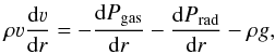$\begin{matrix} ρ ν \frac{d ν}{d r} = - \frac{d P_{gas}}{d r} - \frac{d P_{rad}}{d r} - ρg, \end{matrix}$ $\begin{eqnarray} \label{eq:motion} \rho \varv \frac{\ddif \varv}{\ddif r} = - \frac{\ddif P_{\rm gas}}{\ddif r} - \frac{\ddif P_{\rm rad}}{\ddif r} - \rho g, \end{eqnarray}$ (1)and the equation of continuity 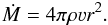$\begin{matrix} Ṁ = 4 πρ ν r^{2} . \end{matrix}$ $\begin{eqnarray} \label{eq:cont} \dot{M} = 4\pi \rho \varv r^2. \end{eqnarray}$ (2)Here P_gas and P_rad are the gas pressure and radiation pressure, and g is the local gravitational acceleration GM/r². The gradient of P_rad in Eq. (1) is related to the (outward directed) radiative acceleration g_rad via 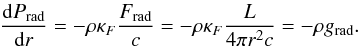$\begin{matrix} \frac{d P_{rad}}{d r} = - ρ κ_{F} \frac{F_{rad}}{c} = - ρ κ_{F} \frac{L}{4 π r^{2} c} = - ρ g_{rad} . \end{matrix}$ $\begin{eqnarray} \label{eq:prad} \frac{\ddif P_{\rm rad}}{\ddif r} = - \rho \kappa_F \frac{F_{\rm rad}}{c} = - \rho \kappa_F \frac{L}{4\pi r^2 c} = - \rho g_{\rm rad}. \end{eqnarray}$ (3)Here F_rad is the frequency-integrated radiative flux 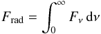$\begin{matrix} F_{rad} = \int_{0}^{\infty} F_{ν} d ν \end{matrix}$ $\begin{eqnarray} \label{eq:flux} F_{\rm rad} = \int_0^\infty F_\nu \dint\nu \end{eqnarray}$ (4)and κ_F the flux-weighted mean opacity $\begin{matrix} κ_{F} = \frac{1}{F_{rad}} \int_{0}^{\infty} κ_{ν} F_{ν} d ν . \end{matrix}$ $\begin{eqnarray} \label{eq:flux-mean} \kappa_F = \frac{1}{F_{\rm rad}} \int_0^\infty \kappa_\nu F_\nu \dint\nu. \end{eqnarray}$ (5)It is important to note that the above equations describe a smooth and stationary gas flow. However, in reality stellar winds are believed to be structured. In this case ρ may indicate a mean density, and κ_F a (spatial) mean opacity that includes effects like clumpiness and porosity of the wind material (cf. Hamann & Koesterke 1998; Oskinova et al. 2007). We wish to emphasize that the following derivations are still valid in this case, i.e. we assume that κ_F includes effects like clumping and porosity.

To estimate the sonic-point optical depth τ_s we make use of the fact that, due to hydrostatic equilibrium in the subsonic region (i.e. for r < R_s), the terms on the right hand side of Eq. (1) cancel each other and become essentially zero. In the supersonic region the situation is different as radiation pressure starts to dominate the dynamics of the gas flow. In this case P_gas can be neglected and after multiplication with 4πr² Eq. (1) becomes $\begin{matrix} 4 πρ ν r^{2} d ν = 4 π r^{2} ρ (g_{rad} - g) d r . \end{matrix}$ $\begin{eqnarray} 4\pi \rho \varv r^2 \dint \varv = 4\pi r^2 \rho~(g_{\rm rad}-g) \dint r. \end{eqnarray}$ (6)With the equation of continuity (Eq. (2)), and the Eddington factor Γ = g_rad/g this equation becomes $\begin{matrix} Ṁ d ν = 4 πGMρ (Γ - 1) d r . \end{matrix}$ $\begin{eqnarray} \dot{M} \dint \varv = 4\pi G M \rho~(\Gamma-1) \dint r. \end{eqnarray}$ (7)Using the definitions in Eq. (3) we obtain for r > R_s $\begin{matrix} \frac{Ṁ}{L / c} d ν = κ_{F} ρ \frac{Γ - 1}{Γ} d r = \frac{Γ - 1}{Γ} d τ \end{matrix}$ $\begin{eqnarray} \frac{\dot{M}}{L/c} \dint \varv = \kappa_F \rho \frac{\Gamma-1}{\Gamma} \dint r = \frac{\Gamma-1}{\Gamma} \dint \tau \end{eqnarray}$ (8)with the flux-mean optical depth τ. Taking into account that the left hand side of Eq. (1) becomes small due to hydrostatic equilibrium below R_s, the integral of (Eq. (1)) × 4πr² becomes $\begin{matrix} \int_{0}^{ν_{\infty}} \frac{Ṁ}{L / c} d ν = \frac{Ṁ ν_{\infty}}{L / c} = \int_{R_{s}}^{\infty} \frac{Γ - 1}{Γ} d τ \approx τ_{s} . \end{matrix}$ $\begin{eqnarray} \int_0^{\varv_\infty} \frac{\dot{M}}{L/c} \dint \varv = \frac{\dot{M}\varv_\infty}{L/c} = \int_{R_{\rm s}}^\infty \frac{\Gamma-1}{\Gamma} \dint \tau \approx \tau_{\rm s}. \end{eqnarray}$ (9)In the last step we assumed that Γ is significantly larger than one in the supersonic region. In reality Γ will, however, only be moderately larger than one, so that we expect that 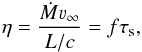$\begin{matrix} η = \frac{Ṁ ν_{\infty}}{L / c} = f τ_{s}, \end{matrix}$ $\begin{eqnarray} \label{eq:taus} \eta = \frac{\dot{M}\varv_\infty}{L/c} = f \tau_{\rm s}, \end{eqnarray}$ (10)with f ≲ 1 (cf. Vink & Gräfener 2012). We can thus gain information about τ_s from the basic stellar/wind parameters Ṁ, ν_∞, and L as they are routinely determined in spectral analyses.

Under optically thick conditions, i.e. for large τ_s, the temperature is connected to τ via the radiative diffusion equation. We can thus gain important information about the sonic-point temperature T_s in otherwise unobservable layers below the photosphere, just by investigating basic stellar/wind parameters.

3.2. The temperature structure in optically thick winds

To estimate the temperature structure T(r) in the sub-photospheric layers of an optically thick wind we compute the radiation pressure P_rad(r) from Eq. (3). We assume that the radiation pressure P_ref at a reference radius R_ref is known, and rewrite Eq. (3) in terms of the radiative flux F_ref at this radius. 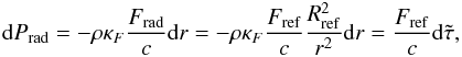$\begin{matrix} d P_{rad} = - ρ κ_{F} \frac{F_{rad}}{c} d r = - ρ κ_{F} \frac{F_{ref}}{c} \frac{R_{ref}^{2}}{r^{2}} d r = \frac{F_{ref}}{c} d \begin{matrix} ˜ \\ τ \end{matrix}, \end{matrix}$ $\begin{eqnarray} \label{eq:dprad} \ddif P_{\rm rad} = -\rho\kappa_F \frac{F_{\rm rad}}{c} \ddif r = - \rho \kappa_F \frac{F_{\rm ref}}{c} \frac{R_{\rm ref}^2}{r^2} \ddif r = \frac{F_{\rm ref}}{c} \ddif \tilde{\tau}, \end{eqnarray}$ (11)with the modified optical depth $\begin{matrix} ˜ \\ τ \end{matrix}$ $\hbox{$\tilde{\tau}$}$ defined by 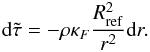$\begin{matrix} d \begin{matrix} ˜ \\ τ \end{matrix} = - ρ κ_{F} \frac{R_{ref}^{2}}{r^{2}} d r . \end{matrix}$ $\begin{eqnarray} \label{eq:taumod} \ddif \tilde{\tau} = - \rho \kappa_F \frac{R_{\rm ref}^2}{r^2} \ddif r. \end{eqnarray}$ (12)F_ref can be computed from the stellar luminosity L and R_ref. We can define an effective temperature (or flux temperature) T_ref related to this radius 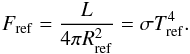$\begin{matrix} F_{ref} = \frac{L}{4 π R_{ref}^{2}} = σ T_{ref}^{4} . \end{matrix}$ $\begin{eqnarray} \label{eq:tref} F_{\rm ref} = \frac{L}{4\pi R_{\rm ref}^2} = \sigma T_{\rm ref}^4. \end{eqnarray}$ (13)With these definitions we can compute P_rad directly from Eq. (11) 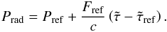$\begin{matrix} P_{rad} = P_{ref} + \frac{F_{ref}}{c} (\begin{matrix} ˜ \\ τ \end{matrix} - {\begin{matrix} ˜ \\ τ_{ref} \end{matrix}}^{)} . \end{matrix}$ $\begin{eqnarray} \label{eq:pradf} P_{\rm rad} = P_{\rm ref} + \frac{F_{\rm ref}}{c} \left(\tilde{\tau} - \tilde{\tau}_{\rm ref}\right). \end{eqnarray}$ (14)This result is exact if the modified optical depth $\begin{matrix} ˜ \\ τ_{ref} \end{matrix}$ $\hbox{$\tilde{\tau}_{\rm ref}$}$ and the radiation pressure P_ref at R_ref are known. Following Lucy & Abbott (1993) we assume that T = T_ref for $\begin{matrix} _{˜} \\ τ_{ref} \end{matrix} = 2 / 3$ $\hbox{$\tilde{\tau}_{\rm ref}=2/3$}$ . Moreover, we adopt $P_{rad} = \frac{4 σ}{3 c} T^{4}$ $\hbox{$P_{\rm rad}=\frac{4\sigma}{3c}T^4$}$ for the optically thick regime and obtain 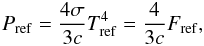$\begin{matrix} P_{ref} = \frac{4 σ}{3 c} T_{ref}^{4} = \frac{4}{3 c} F_{ref}, \end{matrix}$ $\begin{eqnarray} P_{\rm ref} = \frac{4\sigma}{3c}T_{\rm ref}^4 = \frac{4}{3c} F_{\rm ref}, \end{eqnarray}$ (15)and Eq. (14) becomes 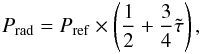$\begin{matrix} P_{rad} = P_{ref} \times (\frac{1}{2} + \frac{3}{4} \begin{matrix} ˜ \\ τ \end{matrix}), \end{matrix}$ $\begin{eqnarray} \label{eq:peq} P_{\rm rad} = P_{\rm ref} \times \left( \frac{1}{2} + \frac{3}{4} \tilde{\tau}\right), \end{eqnarray}$ (16)or 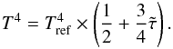$\begin{matrix} T^{4} = T_{ref}^{4} \times (\frac{1}{2} + \frac{3}{4} \begin{matrix} ˜ \\ τ \end{matrix}) . \end{matrix}$ $\begin{eqnarray} \label{eq:teq} T^4 = T_{\rm ref}^4 \times \left(\frac{1}{2} + \frac{3}{4} \tilde{\tau}\right). \end{eqnarray}$ (17)This result is identical to the more general relation from Lucy (1971, 1976) and Lucy & Abbott (1993), for $\begin{matrix} _{˜} \\ τ \end{matrix} > 2 / 3$ $\hbox{$\tilde{\tau} > 2/3$}$ .

3.3. Numerical tests

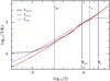Fig. 1

Temperature structure $T (\begin{matrix} _{˜} \\ τ \end{matrix})$ $\hbox{$T(\tilde{\tau})$}$ from the WC star model by Gräfener & Hamann (2005). T_NLTE (black) is the temperature computed in non-LTE within the model, and T_Lucy (red) is obtained from the relation by Lucy & Abbott (1993) which is identical with Eq. (17) for $\begin{matrix} _{˜} \\ τ \end{matrix} > 2 / 3$ $\hbox{$\tilde{\tau} > 2/3$}$ . T_flux (blue dashed) denotes the local flux temperature. The dashed vertical lines indicate the classical photosphere r_ph with a flux-mean optical depth τ = 2/3, and the electron-scattering photosphere r_es with an electron-scattering optical depth τ_es = 2/3. Solid vertical lines indicate the sonic radius R_s and the reference radius R_ref with $\begin{matrix} _{˜} \\ τ \end{matrix} = 2 / 3$ $\hbox{$\tilde{\tau}=2/3$}$ where T_Lucy = T_flux is adopted (cf. Eq. (13)).

To verify the applicability of Eqs. (10) and (17) we use numerical models for the atmospheres/winds of WR stars by Gräfener & Hamann (2005, 2008). These models compute the detailed radiation field in the co-moving frame of reference (CMF) using the method by Koesterke et al. (2002), and solve the equations of radiative and statistical equilibrium in non-LTE to compute the electron temperature T(r) and the atomic level populations n_i(r) (Gräfener et al. 2002; Hamann & Gräfener 2003). ρ(r) and ν(r) are obtained simultaneously with the non-LTE quantities from a precise iterative solution of Eq. (1) using the radiative acceleration g_rad as obtained from an explicit integration of κ_ν × F_ν in Eq. (5) (cf. Gräfener & Hamann 2005).

The numerical models provide ρ(r), ν(r), T(r), and the populations n_i(r) for each atomic energy level i. The latter are used to compute opacities κ_ν(r), emissivities η_ν(r), and the intensity I_ν(μ,r) in the CMF. These quantities are computed on a grid that usually comprises ~10⁵ frequency points, and ~70 grid points in radius r and angle μ. The fluxes F_ν are then obtained by integration of I_ν × μ over μ. κ_F and g_rad are evaluated in the CMF using Eqs. (3)–(5).

We start with the hydrodynamic WC star model from Gräfener & Hamann (2005). This model has a very compact core and high T_⋆. The inner boundary is located at a stellar radius R_⋆ = 0.905 R_⊙ corresponding to T_⋆ = 140 kK for log (L/L_⊙) = 5.45.

To estimate $T (\begin{matrix} _{˜} \\ τ \end{matrix})$ $\hbox{$T(\tilde{\tau})$}$ from Eq. (17) we need to determine T_ref, i.e. we have to find the reference radius R_ref with $\begin{matrix} _{˜} \\ τ_{ref} \end{matrix} = 2 / 3$ $\hbox{$\tilde{\tau}_{\rm ref} = 2/3$}$ . As ρ(r) and κ_F(r) are given within the model, this can be done iteratively by varying R_ref and integrating Eq. (12) until 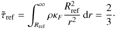$\begin{matrix} \begin{matrix} ˜ \\ τ_{ref} \end{matrix} = \int_{R_{ref}}^{\infty} ρ κ_{F} \frac{R_{ref}^{2}}{r^{2}} d r = \frac{2}{3} \cdot \end{matrix}$ $\begin{eqnarray} \tilde{\tau}_{\rm ref} = \int_{R_{\rm ref}}^\infty \rho\kappa_F\frac{R_{\rm ref}^2}{r^2} \dint r = \frac{2}{3}\cdot \end{eqnarray}$ (18)For given R_ref the flux F_ref and flux temperature T_ref can be computed from Eq. (13). For our example model we find R_ref = 2.28 R_⋆ and T_ref = 92 473 K. This value compares very well with the non-LTE temperature T(R_ref) = 91 976 K as computed from the condition of radiative equilibrium within the model (cf. Fig. 1). This result nicely supports the assumption that T = T_ref for $\begin{matrix} _{˜} \\ τ \end{matrix} = 2 / 3$ $\hbox{$\tilde{\tau}=2/3$}$ .

In Fig. 1 we compare $T (\begin{matrix} _{˜} \\ τ \end{matrix})$ $\hbox{$T(\tilde{\tau})$}$ as computed from Eq. (17) with the non-LTE temperature from the numerical model. In particular in deep atmospheric layers ( $\begin{matrix} _{˜} \\ τ \end{matrix} ≳ 10$ $\hbox{$\tilde{\tau} \gtrsim 10$}$ ) both temperatures agree remarkably well. E.g., at the sonic radius R_s (= 1.03 R_⋆) the agreement is better than 2%. Large differences only occur in the outermost layers, beyond the “classical” photospheric radius r_ph (defined with respect to the flux-mean optical depth τ(r_ph) = 2/3). In our example r_ph is located at 25.0 R_⋆. This is very far out in the wind, but still within the formation region of the strong WR emission lines.

The photosphere defined with respect to the electron scattering opacity κ_es is located below R_ref at r_es = 1.41 R_⋆. r_es is of the same order of magnitude as R_ref, and can be estimated easily using analytical relations e.g. by de Loore et al. (1982). For this reason we will use it in Sect. 4.1 to obtain very coarse, but purely empirical estimates of the sonic point conditions.

3.4. Representation by β-law models

In the remainder of this work we want to investigate WR stars in general, i.e. without having access to radiation-hydrodynamic models as in Sect. 3.3. To this purpose we assume that the winds of our sample stars are radiatively driven, and derive the radiative acceleration g_rad(r) and mean opacity κ_F(r) adopting a β-type velocity distribution 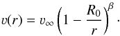$\begin{matrix} ν (r) = ν_{\infty} {(1 - \frac{R_{0}}{r})}^{β} \cdot \end{matrix}$ $\begin{eqnarray} \label{eq:betalaw} \varv(r) = \varv_\infty\left( 1 - \frac{R_0}{r}\right)^\beta\cdot \end{eqnarray}$ (19)Here β is the wind acceleration parameter (usually of the order of one), and R₀ (≈R_⋆) the radius parameter. R₀ is adjusted to connect ν(r) continuously to an exponential velocity law with ν(r) ∝ exp((r − R_⋆)/H) at the inner boundary of the model atmosphere. We note that in some cases R_s may be located in the exponential regime, so that the adopted scale height H may influence our results.

To infer the sonic-point conditions in an analogous way as in Sect. 3.3, we compute ν (dν/dr) from the given velocity structure ν(r), and compute the flux-mean opacity κ_F(r) which is consistent with ν(r) from Eqs. (1) and (3). This is easily possible as the gas pressure gradient dP_rad/ dr in Eq. (1) is nearly negligible in the supersonic region, i.e. it could be set to zero. Nevertheless we compute P_gas for the temperature resulting from Eq. (17), and correct for it in an iterative way.

We apply this method to a model that resembles the properties of the hydrodynamic model from Sect. 3.3 but uses a velocity law with β = 1 (model D from Gräfener & Hamann 2005). In particular, the model has (almost) the same wind efficiency η = 2.5 as the hydrodynamic model. The resulting optical-depth scales and sonic-point conditions for the two models are given at the bottom of Table 2.

Although the velocity structure of the hydrodynamic model is significantly different from a β-type velocity law (cf. Fig. 8 in Gräfener & Hamann 2005) we obtain a very similar wind optical depth τ_s(≈10) as for the hydrodynamical model. Consequently the correction factor f in Eq. (10) is almost identical for both models, and the sonic-point conditions are almost the same. For the hydrodynamic model we find R_s = 1.027 R_⋆ and T_s = 195 160 K, and for the β-law model R_s = 1.021 R_⋆ and T_s = 201 817 K. This result is in line with Vink & Gräfener (2012) who found that the correction factor f mainly depends on the ratio ν_∞/ν_esc, and not on the detailed velocity structure. For our upcoming analysis in Sect. 4 we will thus adopt β-type velocity distributions.

4. Application to Galactic WC stars

Here we apply the methods described in Sect. 3 to a large sample of WC stars. WC stars are the naked cores of massive stars that have been stripped off their H-rich layers during their previous evolution. They show the products of He-burning at their surface (e.g. Gräfener et al. 1998) and have particularly strong optically thick winds. The vast majority of these stars is believed to be in the phase of core He-burning, with only very few cases in later burning stages just before a supernova explosion (this class of objects may be represented by the minority of WO stars; cf. Yoon et al. 2012). Due to the strong temperature-sensitivity of He-burning, WC stars are expected to have very similar core temperatures and will thus follow a well-defined mass-luminosity relation (Langer 1989).

The complete sample of Galactic WC and WO stars with available optical spectroscopy has recently been analysed by Sander et al. (2012). Here we use the stellar/wind parameters (i.e. luminosities L, stellar temperatures T_⋆, mass-loss rates Ṁ, and terminal wind velocities ν_∞) of the 45 putatively single WC/WO stars from this work, combined with results for Galactic and LMC WC/WO stars by Hillier & Miller (1999), De Marco et al. (2000), Dessart et al. (2000), Smartt et al. (2001), Crowther et al. (2006), Crowther et al. (2002), Crowther et al. (2000), Gräfener et al. (2002), Gräfener & Hamann (2005) which are based on atmosphere models including Fe line-blanketing. In total we have a sample of 61 sets of stellar/wind parameters for WC stars for which masses can be obtained from the mass-luminosity relation by Langer (1989).

For this parameter set we estimate sonic-point densities and temperatures as described in the previous section. In Sect. 4.1 we start with a very coarse but almost purely empirical approach to compute the sonic-point conditions. Then we continue in Sect. 4.2 with a more detailed analysis that is based on numerical models as described in Sect. 3.4.

4.1. Semi-empirical estimates of the sonic point conditions

To obtain the sonic-point temperature T_s = T(R_s) from Eq. (17) we need to determine T_ref and $\begin{matrix} _{˜} \\ τ_{s} \end{matrix} = \begin{matrix} _{˜} \\ τ \end{matrix} (R_{s})$ $\hbox{$\tilde{\tau}_{\rm s} = \tilde{\tau}(R_{\rm s})$}$ . Here we start with a simplified, but purely empirical method to estimate these quantities. To this purpose we assume that the reference radius R_ref is of the same order of magnitude as the radius of the electron-scattering photosphere r_es where τ_es = 2/3 (cf. Sect. 3.3). τ_es can be computed analytically. Using the relations by de Loore et al. (1982) we give τ_es in Eqs. (20) and (21) using the parameter C = Ṁ/(R_⋆ν_∞) which is proportional to the product of wind density and stellar radius. Furthermore τ_es is proportional to the electron scattering opacity κ_es = (0.22 cm²/g) × (1 + X), where we assume a fully ionized plasma with hydrogen mass fraction X. For a given value of β ≠ 1 and F = r_es/R_⋆ the condition τ_es = 2/3 then reads $\begin{matrix} τ_{es} = - κ_{es} C (1 - β) [{(1 - 1 / F^{)}}^{1 - β} - 1^{]} = 2 / 3, \end{matrix}$ $\begin{eqnarray} \label{eq:taues_beta} \tau_{\rm es} = - \kappa_{\rm es} C (1-\beta) \left[\left(1-1/F\right)^{1-\beta} -1\right] = 2/3, \end{eqnarray}$ (20)and for β = 1 $\begin{matrix} τ_{es} = - κ_{es} C \ln (1 - 1 / F) = 2 / 3. \end{matrix}$ $\begin{eqnarray} \label{eq:taues1} \tau_{\rm es} = - \kappa_{\rm es} C \ln(1-1/F) = 2/3. \end{eqnarray}$ (21)In Table 1 we list estimates of wind parameters based on this approach. They are determined in the following way. T_ref is computed from Eq. (13) assuming that R_ref = r_es using F = r_es/R_⋆ from Eq. (21). $\begin{matrix} ˜ \\ τ_{s} \end{matrix}$ $\hbox{$\tilde{\tau}_{\rm s}$}$ is approximated by $\begin{matrix} _{˜} \\ τ_{s} \end{matrix} \approx τ_{s} \times F^{2}$ $\hbox{$\tilde{\tau}_{\rm s} \approx \tau_{\rm s} \,\times\, F^2$}$ , and the correction factor f in Eq. (10) is approximated by $f ~ \frac{Γ - 1}{Γ} ~ \frac{ν_{\infty} / ν_{esc}}{ν_{\infty} / ν_{esc} + 1}$ $\hbox{$f\sim \frac{\Gamma-1}{\Gamma}\sim\frac{\varv_\infty/\varv_{\rm esc}}{\varv_\infty/\varv_{\rm esc}+1}$}$ (cf. Vink & Gräfener 2012). This leads to 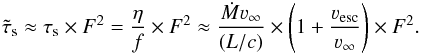$\begin{matrix} \begin{matrix} ˜ \\ τ_{s} \end{matrix} \approx τ_{s} \times F^{2} = \frac{η}{f} \times F^{2} \approx \frac{Ṁ ν_{\infty}}{(L / c)} \times (1 + \frac{ν_{esc}}{ν_{\infty}}) \times F^{2} . \end{matrix}$ $\begin{eqnarray} \tilde{\tau}_{\rm s} \approx \tau_{\rm s} \times F^2 = \frac{\eta}{f}\times F^2 \approx \frac{\dot{M}\varv_\infty}{(L/c)} \times \left(1 + \frac{\varv_{\rm esc}}{\varv_\infty}\right) \times F^2. \end{eqnarray}$ (22)At this point we have expressed $\begin{matrix} ˜ \\ τ_{s} \end{matrix}$ $\hbox{$\tilde{\tau}_{\rm s}$}$ by quantities that are determined in spectral analyses. Based on $\begin{matrix} ˜ \\ τ_{s} \end{matrix}$ $\hbox{$\tilde{\tau}_{\rm s}$}$ we then obtain T_s from Eq. (17), and ρ_s from Eq. (2) assuming that r_s ≈ R_⋆. From T_s and ρ_s we compute the gas pressure P_gas and radiation pressure P_rad at the sonic point assuming a mean molecular weight μ = 4/3. The resulting values are listed in Table 1 and plotted in Fig. 2. Please note that we have inverted the axes in Fig. 2 so that the lower left corner of the plot corresponds to high densities and temperatures as they are found deep inside the stellar envelope, while the upper right corner corresponds to layers further outside.

In Fig. 2 it can be seen that all stars in our sample follow a relation with log (P_rad/P_gas) ≈ 2, i.e. at the sonic point radiation pressure generally dominates gas pressure roughly by a factor 100. The existence of such a relation is surprising as our sample contains a variety of WC/WO subtypes with very different wind properties and metallicities. This relation may thus be a ubiquitous property of optically thick winds.

The temperature and density estimates obtained in the present section are approximative but based on universal relations. The only place where the detailed velocity structure goes in (in the form of the parameter β) is the computation of R_ref based on Eq. (21). A main source of uncertainty may be the assumption that R_ref = r_es. In our example in Sect. 3.3 we have seen that R_ref > r_es. The reference temperatures T_ref, and consequently also the sonic point temperatures T_s obtained in this section are thus likely too high.

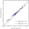Fig. 2

Sonic-point conditions for our sample of putatively single WC/WO stars in the Galaxy and LMC. Density and temperature at the sonic point are expressed in terms of gas and radiation pressure P_gas and P_rad. Blue crosses indicate results from our empirical analysis in Sect. 4.1, black dots indicate estimates based on β-type wind models from Sect. 4.2. Both methods indicate a sonic-point relation with P_rad/P_gas = const. Uncertainties for the semi-empirically determined data points are discussed in Sect. 5.3. For the ratio of P_rad/P_gas they are likely of the order of 0.3 dex, but may be higher for individual positions along the indicated relations.

4.2. Numerical estimates

In this section we use the numerical modelling approach described in Sect. 3.4 to estimate the sonic-point conditions for our sample stars. We adopt a β-type velocity law (Eq. (19)) with β = 1 for ν(r) and compute all optical depth scales using the opacity κ_F(r) that is consistent with the corresponding wind acceleration ν(dν/dr), i.e. we assume that the winds are radiatively driven.

The results are listed in Table 2 and plotted in Fig. 2 in the same form as the results from Sect. 4.1. With the numerical method the relation from Sect. 4.1 is retained, but the obtained temperatures are lower because the reference radii R_ref are larger than r_es. Consequently the relation for P_rad/P_gas shifts by ~0.2 dex with respect to the data points from Sect. 4.1. In view of the large differences between both approaches this demonstrates the robustness of this result.

As we will discuss later, the relation for P_rad/P_gas obtained in this way imposes a boundary condition on the stellar envelope at the sonic point. More precisely, it reflects a boundary condition that is imposed by the presence of an optically thick, radiatively driven wind. According to our present semi-empirical results this “wind condition” has the form $\begin{matrix} \frac{P_{rad}}{P_{gas}} \approx 80. \end{matrix}$ $\begin{eqnarray} \label{eq:sonic} \frac{P_{\rm rad}}{P_{\rm gas}} \approx 80. \end{eqnarray}$ (23)

5. An artificial model sequence for WC/WO stars

In order to investigate the general applicability of our results, as well as their sensitivity to uncertainties in the observed stellar parameters, we construct a model sequence for WC/WO stars that is suitable for a systematic analysis. To this purpose we introduce the concept of the transformed mass-loss rate Ṁ_t in Sect. 5.1. In Sect. 5.2 we discuss the observed properties of WC/WO stars and define an artificial WC/WO sequence. In Sect. 5.3 we vary input parameters and model assumptions to investigate the reliability of our method.

5.1. The transformed mass-loss rate

A remarkable property of massive WC stars is their homogeneous spectroscopic appearance. For a given spectral subtype (i.e. for given T_⋆) their normalized spectra are almost invariant regardless of their luminosity. The stellar/wind parameters of WC stars thus follow a scaling relation which preserves the equivalent widths of their emission lines for given T_⋆. If the luminosity L (or equivalently the radius R_⋆) are changed, this scaling relation has to ensure that the wind parameters (mass-loss rate Ṁ, terminal wind speed ν_∞ and clumping factor D) are adapted in a way that the line equivalent widths stay constant.

Based on numerical results, such a scaling relation has been introduced by Schmutz et al. (1989) via the so-called transformed radius R_t. This parameter is of large benefit for the analysis of emission-line stars as it reduces the number of free parameters by two, and enables a two-step analysis where the normalized spectrum is modeled in step one, and the flux-distribution (including interstellar extinction) in step two.

Hamann & Koesterke (1998) explained this invariance with the dominance of recombination processes for the line emission in WR stars. As recombination is an n² process, the line emissivity j per unit volume scales with j ∝ n², and its spatial mean goes with $\hbox{$\bar{j}\propto n^2/D$}$ if clumping is taken into account (cf. Sect. 2.2). The observed line flux F_l is given by the product of the mean emissivity and the line-emitting volume, i.e. $\hbox{$F_{\rm l} \propto \bar{j} \times V$}$ . At this point Hamann & Koesterke (1998) assumed that $V \propto R_{⋆}^{3}$ $\hbox{$V\propto R_\star^3$}$ , i.e. the radial size Δr of the line-emitting region in the spherically symmetric wind scales as Δr = Δr′ × R_⋆ with Δr′ = const. Here we show that this assumption is indeed correct if Δr is determined by photoionization equilibrium. In this case the ionization rate is balanced by the recombination rate, i.e. F × n_s ∝ n², where F denotes the ionizing flux, n_s the density of the subordinate ionization stage, and n the density of the main ionization stage (which is almost equal to the total particle density). If we adopt a radial scaling with r = r′ × R_⋆, then F(r′) is invariant if also the optical depth τ(r′) ∝ n_s(r′) × Δr/D in the ionizing continuum is preserved. With the scaling relations for Δr and n_s from above this relation becomes τ(r′) ∝ n_s(r′) × Δr/D ∝ n²(r′) × R_⋆/D = const. To preserve the optical depth scale τ(r′) we thus need to fulfill the scaling relation n²(r′) × R_⋆/D = const.

Notably, in this case we have $F_{l} \propto j̅ \times V \propto n^{2} (r^{'}) \times R_{⋆}^{3} / D \propto R_{⋆}^{2}$ $\hbox{$F_{\rm l} \propto \bar{j} \times V \propto n^2(r') \times R_\star^3/D \propto R_\star^2$}$ . The line flux $F_{l} \propto R_{⋆}^{2}$ $\hbox{$F_{\rm l}\propto R_\star^2$}$ thus scales in the same way with the stellar radius as the luminosity $L \propto R_{⋆}^{2}$ $\hbox{$L\propto R_\star^2$}$ , i.e. line equivalent widths are preserved. To express this scaling relation in terms of standard wind parameters we use Eqs. (2) and (19), i.e. $Ṁ \propto n (r^{'}) ν (r^{'}) r^{2} / D \propto n (r^{'}) ν_{\infty} R_{⋆}^{2} / D$ $\hbox{$\dot{M} \propto n(r') \varv(r') r^2/D \propto n(r') \varv_\infty R_\star^2/D$}$ . This finally leads to $n^{2} (r^{'}) \times R_{⋆} / D \propto (Ṁ / ν_{\infty})^{2} R_{⋆}^{3} D = const .$ $\hbox{$n^2(r') \times R_\star /D \propto (\dot{M}/\varv_\infty)^2 R_\star^3 D={\rm const}.$}$ In the following we express this scaling relation via the transformed mass-loss rate $\begin{matrix} Ṁ t = Ṁ \sqrt{D} \times (\frac{1000 {km s}^{-1}}{ν_{\infty}}) {(\frac{10^{6} L_{⊙}}{L})}^{3 / 4} \cdot \end{matrix}$ $\begin{eqnarray} \label{eq:mtrans} \dot{M}_{\rm t} = {\dot{M} \sqrt{D}} \times {\left(\frac{1000\,{\rm km\,s}^{-1}}{\varv_\infty}\right) \left(\frac{10^6 L_\odot}{L}\right)^{3/4}}\cdot \end{eqnarray}$ (24)For a star with given emission line equivalent widths Ṁ_t denotes the mass-loss rate that the star would have if it had L = 10⁶ L_⊙, ν_∞ = 1000 km s, and D = 1. We note that this definition is fully equivalent to the relation resulting from the transformed radius R_t as introduced by Schmutz et al. (1989); Hamann & Koesterke (1998). In the context of our present work Ṁ_t is, however, more meaningful as it is directly related to the stellar mass-loss rate.

5.2. Stellar/wind parameters of WC/WO stars

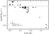Fig. 3

Transformed mass-loss rates Ṁ_t (Eq. (24)) versus stellar temperatures T_⋆ for our sample of putatively single WC (circles) and WO stars (squares). Filled symbols indicate objects in the Galaxy, empty symbols objects in the LMC. Some symbols have been shifted to avoid overlaps. The grey dashed line indicates the transformed mass-loss rate adopted for our artificial model sequence.

In Fig. 3 we plot Ṁ_t vs. T_⋆ for the stars in our sample. Notably, the Galactic WC stars are lying in a regime with log (Ṁ_t) ≈ − 4 (in M_⊙ yr^-1), with a tendency of slightly higher mass-loss rates for late subtypes. This relation is equivalent to the relation for the transformed radius R_t with $R_{t} \propto T_{⋆}^{-2}$ $\hbox{$R_{\rm t}\propto T_\star^{-2}$}$ from Barniske et al. (2006); Sander et al. (2012). Only the extremely hot Galactic WO stars form a separate group with much lower log (Ṁ_t) ≈ − 5.

The LMC WC stars have slightly lower Ṁ_t than the Galactic ones, and the only LMC WO star is located somewhat between the Galactic WC and WO stars.

Based on the few WO stars and the slight excess for late subtypes, Fig. 3 may even suggest a steep decrease of Ṁ_t with increasing T_⋆. It is, however, not clear whether this decrease is related to a metallicity dependence of WR mass-loss (as theoretically predicted by Vink & de Koter 2005; Gräfener & Hamann 2008), or if it is an intrinsic property of WC/WO stars. Observationally, late WC subtypes are mainly found in high-metallicity environments, while early subtypes dominate at low metallicities as in the LMC. In any case most Galactic WC stars comply with log (Ṁ_t) ≈ − 4 as indicated by the dashed grey line in Fig. 3. In the following we adopt this value for our artificial model sequence.

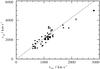Fig. 4

Terminal wind velocities ν_∞ vs. escape velocities ν_esc for our sample of WC/WO stars. Symbols are the same as in Fig. 3. Typical uncertainties are of the order Δν_∞ = ± 10% and Δν_esc = ± 15%. The grey dashed line indicates the relation with ν_∞/ν_esc = 1.6 as adopted for our artificial model sequence.

In Fig. 4 we plot ν_∞ vs. ν_esc for our sample stars. While ν_∞ can be inferred directly from the observed blue edges of P-Cygni absorption troughs, ν_esc is determined from the stellar luminosity L and temperature T_⋆ as obtained from spectral analyses. Based on these two quantities we compute the radii R_⋆. The stellar masses M follow from L, and to a lesser extent from the obtained/adopted surface abundances, using the relation from Langer (1989). The resulting escape velocities $ν_{esc} = \sqrt{2 GM / R_{⋆}}$ $\hbox{$\varv_{\rm esc} = \sqrt{2GM/R_\star}$}$ are listed together with the other stellar parameters in Table 2. Figure 4 clearly suggests a relation between ν_∞ and ν_esc². Again, this picture may be complicated by a possible dependence on metallicity (cf. Gräfener & Hamann 2008), and the low numbers of extremely compact WO stars. For our artificial model sequence we adopt ν_∞/ν_esc ~ 1.6 as indicated by the dashed grey line in Fig. 4.

We note that the existence of a relation with ν_∞/ν_esc = const. is plausible as it implies that the mechanical wind energy is of a similar order of magnitude as the gravitational wind energy (cf. Sect. 6.1). The observed relation in Fig. 4 thus supports the existence of a broad range of gravitational energies for WC/WO stars. This means that the stellar radii also span a broad range, in accordance with the R_⋆ obtained from spectral analyses. In contrast, theoretically predicted values (e.g. by Langer 1989) span a much narrower range. The observed relation in Fig. 4 thus supports our scenario 2) from Sect. 2.4 where the spectroscopically determined radii reflect the actual surface radii, and the sub-surface layers of many WC stars are substantially inflated.

5.3. Dependence on stellar/wind parameters

As the obtained sonic-point relation (Eq. (23)) depends on stellar parameters as input, we investigate here its sensitivity to uncertainties in these parameters.

Apart from ν_∞ which can be reliably determined from observed UV line profiles, most of our “input” stellar parameters (Ṁ, L, and T_⋆) rely on numerical modelling and may suffer from systematic uncertainties. While uncertainties in the empirical mass-loss rates Ṁ are probably dominated by the effects of clumping and porosity (cf. Sect. 2.2), L and T_⋆ may suffer from uncertainties in the model physics, mainly due to the (in)completeness of the included atomic data. In the past, Fe-group line blanketing turned out to affect the overall flux distribution and temperature of WR model atmospheres considerably. Since its inclusion in modern non-LTE codes (Hillier & Miller 1998; Gräfener et al. 2002) quantitative results, however, seem to converge.

To investigate the sensitivity of our results to uncertainties and/or changes in stellar parameters, we construct an artificial model sequence with the properties discussed in Sect. 5.2, i.e. with log (Ṁ_t/(M_⊙ yr^-1)) = −4 and ν_∞/ν_esc = 1.6. We cover a temperature range of log (T_⋆/K) = 4.5 ... 5.3 in steps of 0.1 dex and use a typical luminosity for WC stars of log (L/L_⊙) = 5.5 (e.g. Sander et al. 2012). We note that wind clumping has no direct effect on our modelling approach, but it affects the mass-loss rates Ṁ that follow from Eq. (24). Here we adopt a clumping factor of D = 10. For the velocity distribution we adopt a β-law with β = 1 which is smoothly connected to an exponential law with a fixed density scale height H in the hydrostatic layers (cf. Sect. 3.4). H is computed for r = R_⋆, T = T_⋆, and M_eff = M(1 − Γ) with Γ = 0.9. In the following we investigate the effects of changes in Ṁ, L, ν_∞, β, and H.

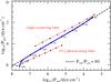Fig. 5

Sonic-point conditions for our artificial model sequence for WC/WO stars. The blue line indicates the sequence of reference models (also denoted as “reference sequence”). Labels indicate stellar temperatures T_⋆ along the reference sequence. The black dashed line indicates the wind condition according to Eq. (23). Red dotted lines indicate relevant mass-loss limits (see text).

In Fig. 5 we show the inferred sonic-point conditions for our reference models. First of all, the reference models form a sequence that reaches from low P_rad for the coolest models to high P_rad for the hottest models. In the following we denote this sequence as the “reference sequence”. Notably, 8 of the 9 models from the reference sequence lie almost precisely on a straight line with P_rad/P_gas = 80, in agreement with the wind condition Eq. (23). Furthermore, Fig. 5 shows two model sequences for which the mass-loss rates have been adjusted to match relevant mass-loss limits, namely the single-scattering limit (η = Ṁν_∞/(L/c) = 1) and 50% of the photon-tiring limit (L_wind = L/2).

As η ≈ τ_s according to Eq. (10), the single-scattering limit marks the mass-loss rate for which the wind becomes optically thin, i.e. 1) the star does not appear as a WR star anymore; and 2) our method is not applicable. Because the τ_s in these test models are smaller than for our reference models, their sonic-point temperatures T_s are smaller and the sequence shifts towards lower values of P_rad.

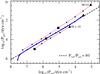Fig. 6

Influence of Ṁ on the sonic-point conditions. The reference sequence (solid blue line) is compared to two test sequences for which the mass-loss rates have been varied by a factor 10 (red dotted lines). Although the models span a factor of 100 in Ṁ the changes with respect to the wind condition Eq. (23) (black dashed line) are moderate. To illustrate the shift in T_⋆, wind models with T_⋆ = 79 kK are indicated by squares and wind models with T_⋆ = 32 kK by triangles.

The photon-tiring limit marks an upper limit for the mass-loss rates of stationary radiatively driven winds (e.g. Owocki et al. 2004; van Marle et al. 2009). It is reached when the (mechanical + gravitational) wind luminosity equals the radiative luminosity of the star, i.e. $L_{wind} = Ṁ \times (ν_{\infty}^{2} / 2 + MG / R_{⋆}) = L$ $\hbox{$L_{\rm wind} = \dot{M} \times (\varv_\infty^2/2 + MG/R_\star) = L$}$ . In this case the radiative luminosity present at R_⋆ would be completely transformed into wind energy and the star would appear dark for the observer. At this point our models would fail. In Fig. 5 we thus indicate 50% of the photon-tiring limit, in which case L_wind = L/2, i.e. the radiative luminosity is significantly reduced within the model. As the temperature is sustained by radiative heating it is substantially reduced in this case, and falls below the value expected from Eq. (23). This is the reason why our hottest reference model deviates from the standard wind condition in Fig. 5.

In Figs. 6–10 we demonstrate the effects of the previously discussed parameter changes on the sonic-point conditions. The strongest effects are caused by changes in Ṁ and ν_∞, which is plausible as they directly affect τ_s via Eq. (10).

In Fig. 6 we compare the reference sequence with two test sequences for which Ṁ (and thus also Ṁ_t) has been changed by a factor 10. All other parameters are kept fixed. It is remarkable that individual models are predominantly shifted along the sonic-point relation. Models with different mass-loss rates thus experience strong changes in T_s but only a moderate shift with respect to Eq. (23) (~0.3 dex). We note that the test performed here is limited, as the 4 hottest models for high Ṁ are in conflict with the photon-tiring limit, and the 4 coolest models for low Ṁ are below the single-scattering limit.

In Fig. 7 we vary the velocity structure by changing ν_∞, keeping Ṁ_t (and thus the wind density) and all other other parameters fixed. We compare three test sequences with ν_∞ = 1000 km s^-1, 2000 km s^-1, and 4000 km s^-1 to the reference sequence. Only for hot models the test sequences do deviate significantly from the reference sequence. The models with ν_∞ = 1000 km s^-1 deviate most. In reality such low values of ν_∞ are not observed for early-type WC or WO stars, so that the expected deviations from Eq. (23) will be small.

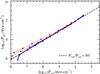Fig. 7

Influence of ν_∞ on the sonic-point conditions. The reference sequence (solid blue line) is compared to test sequences with ν_∞ = 1000 km s^-1, 2000 km s^-1, and 4000 km s^-1 (red dotted lines).

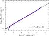Fig. 8

Influence of the adopted luminosity L on the sonic-point conditions. The reference sequence (solid blue line) is compared to test sequences with log (L/L_⊙) = 5 and log (L/L_⊙) = 6 (red dotted lines).

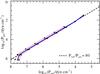Fig. 9

Influence of the adopted acceleration parameter β (Eq. (19)) on the sonic-point conditions. The reference sequence (solid blue line) is compared to test sequences with β = 0.5 and β = 2 (red dotted lines).

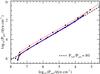Fig. 10

Influence of the density scale height H on the sonic-point conditions. Here we have varied the adopted Eddington parameter Γ which has been used to compute H. The reference sequence with Γ = 0.9 (solid blue line) is compared to test sequences with Γ = 0.5, 0.99, and 0.999 (red dotted lines). A significant effect only occurs for Γ = 0.999.

The tests for changes in L, β, and H are shown in Figs. 8–10. The effects on the sonic-point conditions turn out to be very small in all three cases. In Fig. 8 log (L/L_⊙) has been varied between 5.0 and 6.0, corresponding to the observed range of WC/WO luminosities in the Galaxy and LMC. For both luminosities Ṁ has been adapted to keep Ṁ_t constant. In Fig. 9β has been varied between 0.5 and 2.0, and in Fig. 10 the Eddington factor Γ that is used to compute the density scale height H has been varied between 0.5 and 0.999. Only for the most extreme case of Γ = 0.999 is a significant effect visible, i.e. when H is artificially increased by a factor 10⁴.

The observational uncertainties in our sample from Sect. 4 are dominated by the poorly known distances in the Galaxy resulting in an uncertainty of Δlog (L) = ± 0.3. Here we have shown that our result for P_rad/P_gas is particularly insensitive to variations L. The largest uncertainties in P_rad/P_gas are likely due to uncertainties in Ṁ due to wind clumping. For WR stars these may be of the order of 2–3, i.e. still only a fraction of the factor 100 that we have investigated in Fig. 6. The resulting uncertainty in P_rad/P_gas will be of the order of 0.15 dex. The overall uncertainty in P_rad/P_gas e.g. for the data points in Fig. 2 will probably not exceed 0.3 dex.

We conclude that the wind condition Eq. (23) is insensitive to parameter variations within a realistic range. This means that the existence of an optically thick wind confines the sonic-point conditions to a narrow strip in the P_rad–P_gas plane, in agreement with our semi-empirical results from Sect. 4. Moreover, we find that the photon-tiring limit puts constraints on the earliest WC/WO subtypes.

6. Discussion

Here we discuss the relevance of our results for the winds and the sub-surface structure of stars near the Eddington limit. We start with a discussion of the photon-tiring effect in Sect. 6.1, as it seems to set constraints on the winds of compact WR stars. In Sect. 6.2 we discuss in detail how the wind condition Eq. (23) constrains the winds and sub-surface layers near the Eddington limit.

6.1. Relevance of the photon-tiring limit for WR stars

The photon-tiring limit is reached when the (mechanical plus gravitational) wind luminosity becomes equal to the radiative luminosity of the star, i.e. all photons are used up to drive the wind. The photon-tiring effect is included in quantitative atmosphere/wind models, and has been identified to play a role for the strong winds of WC stars. For quantitative WC models with un-clumped winds Gräfener et al. (1998) found that around 30% of the stellar luminosity are lost to the wind. Since the advent of wind clumping the empirical mass-loss rates have been reduced so that now only ~10% of the stellar luminosity go into the wind (e.g. Crowther et al. 2002).

For our artificial model sequence in Sect. 5 we found that the most compact WR stars are affected by the photon-tiring effect. The reason is that the wind luminosity depends on the gravitational well that has to be overcome by the stellar wind. The mechanical wind luminosity $L_{mech} = (1 / 2) Ṁ ν_{\infty}^{2}$ $\hbox{$L_{\rm mech}=(1/2)\dot{M}\varv_\infty^2$}$ will thus be of the same order of magnitude as the gravitational wind luminosity 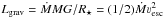$L_{grav} = Ṁ MG / R_{⋆} = (1 / 2) Ṁ ν_{esc}^{2}$ $\hbox{$L_{\rm grav}=\dot{M}MG/R_\star=(1/2)\dot{M}\varv_{\rm esc}^2$}$ . It is thus plausible to assume that ν_∞/ν_esc ≈ const., as we did for our model sequence in Sect. 5.

For the optically thin winds of OB stars relations with ν_∞/ν_esc = const. are theoretically predicted by Castor et al. (1975), with a constant ratio that depends on the atomic properties of the dominating ions in the wind. This is observationally supported e.g. by Lamers et al. (1995) who found ratios of 1.3 and 2.6 for different temperature regimes in the OB star range. For WR stars Niedzielski & Skorzynski (2002) found an increase in ν_∞ for earlier WR subtypes, which is in line with our adopted relation in Sect. 5. In contrast to this Nugis & Lamers (2000) found ν_∞/ν_esc ~ 1 for H-poor WN stars, and varying ν_∞/ν_esc ≲ 1 for WC stars, with strongly deviating values for WO stars. Nugis & Lamers, however, employed the small WR radii as predicted from classical stellar structure models, i.e. they did not consider the possibility of an envelope inflation. Our present results and the ones from Niedzielski & Skorzynski (2002) are based on observed temperatures and radii, and seem to give a more consistent picture over the complete WC/WO regime.

With our assumption that ν_∞/ν_esc = 1.6 we obtain 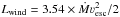$L_{wind} = 3.54 \times Ṁ ν_{esc}^{2} / 2$ $\hbox{$L_{\rm wind}=3.54 \times \dot{M}\varv_{\rm esc}^2/2$}$ . For this case we find that the hottest models in our sequence are affected by the photon tiring effect. The observed stars in this regime are all members of the WO subclass and have ~10 × lower transformed mass-loss rates Ṁ_t than the ones adopted in our models. The underlying reason for the observed mass-loss reduction may thus be related to the photon-tiring effect.

As the formation of WR-type winds is not yet fully understood it is not clear how such a mechanism would work in detail. Ways to reduce the photon tiring effect are, however, 1) a reduction of Ṁ; 2) a reduction of ν_∞; and 3) an increase of R_⋆ through envelope inflation. Following our discussion above, a reduction of ν_∞ may be difficult to realize in nature as it would require that L_mech ≪ L_grav. Compact WC stars may thus be in a situation where photon-tiring forces them to either reduce their mass-loss rates, as observed for the WO subclass, or to increase their radii so that a high mass-loss rate can be maintained. In this case they would appear as normal WC subtypes.

6.2. Relevance for the theory of optically thick winds

The theory of optically thick winds is mainly based on critical point analyses (Pistinner & Eichler 1995; Nugis & Lamers 2002). It is assumed that in the deep layers of optically thick winds the flux-mean opacity κ_F equals the Rosseland mean opacity κ_Ross(ρ,T), so that the radiative acceleration is given as a function of density and temperature g_rad(ρ,T) = κ_Ross(ρ,T)F_rad/c (cf. Eq. (3)). It can be shown that in this case the Eddington limit has to be crossed almost precisely at the sonic point, i.e. the opacity at R_s has to match the value of the Eddington opacity κ_Edd = 4πcGM/L (cf. Sect. 4.1 in Nugis & Lamers 2002). Furthermore, as the wind has do be accelerated outward beyond the sonic point, the opacity has to increase outward, i.e. with decreasing temperature. The sonic-point conditions are thus limited to a curve in ρ–T space for which κ_Ross(ρ,T) = κ_Edd, or more precisely to the branches of this curve with ∂κ_Ross/∂T < 0. This general picture has been confirmed by numerical wind models from Gräfener & Hamann (2005, 2008).

The wind condition Eq. (23) for the ratio between P_rad and P_gas at R_s is highly relevant in this context. The condition that κ_Ross(ρ,T) = κ_Edd can be mapped into the P_rad–P_gas plane, i.e. we have two conditions for P_gas and P_rad that restrict the sonic-point conditions to the intersection points between Eq. (23) and the condition that κ_Ross(P_gas,P_rad) = κ_Edd. On top of this ∂κ_Ross/∂T < 0 has to be fulfilled, and even more importantly, the sonic radius R_s of our wind solution has to match the stellar radius. This last condition over-determines the problem, i.e. we are in need of an additional free parameter to obtain a solution.

A solution to this problem may be given by the envelope inflation effect where the stellar radius becomes a function of the clumping parameter D in the sub-photospheric layers. In this picture a compact WR star may not be able to launch a stationary stellar wind because the sonic-point conditions cannot be fulfilled for the given radius. The result may be a failed wind, i.e. material would be accumulated in shells. Due to the higher density in these shells the mean opacity would increase³ and lead to an increase in the envelope inflation (cf. Gräfener et al. 2012a).

At the moment where the stellar radius enters a range for which a stationary wind solution can be connected the system becomes quasi-stationary with a clumped sub-photospheric structure that sustains a large stellar radius and a wind solution that matches ρ, T, and R of the inflated envelope.

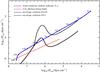Fig. 11

Conditions at the sonic point for a 14 M_⊙ helium star with Galactic metallicity. The solid and dashed black lines indicate stellar envelope solutions with different clumping factors D = 1 and 16 in the sub-surface layers. The conditions imposed by the optically thick stellar wind are indicated in blue. Labels indicate the stellar temperature T_⋆ of the wind solutions. The red dotted line indicates 50% of the photon-tiring limit, i.e. the region where half of the stellar luminosity L is consumed to drive the stellar wind.

In Fig. 11 we visualize this scenario using hydrostatic envelope solutions from Gräfener et al. (2012a). The stellar structure models are computed for a mass of 14 M_⊙ (log (L/L_⊙) = 5.43), and a composition with pure helium and Galactic metallicity of Z = 0.02. The envelope solutions follow a very similar relation with κ_Ross(P_gas,P_rad) ≈ κ_Edd as imposed by the critical point conditions for optically thick winds. The reason is that envelope solutions approaching the Eddington limit cannot exceed it and thus have to stay near the Eddington limit. To obtain a consistent envelope/wind solution we thus have to match the envelope solution to our wind condition Eq. (23). At the same time the radii of the envelope and wind solution have to match each other at the connection point, and we have to fulfill ∂κ_Ross/∂T < 0 which is equivalent to ∂κ_Ross/∂P_rad < 0.

Let us first discuss the envelope solution without clumping (i.e. with D = 1) as indicated by the black curve in Fig. 11. Starting at high P_gas and P_rad (i.e. high ρ and T) in the deep layers of the envelope the solution proceeds to low P_gas and P_rad at the stellar surface. At log (P_rad) ~ 6.2 the solution has a “knee” where it goes to low P_gas (i.e. low densities) and then returns to higher P_gas through an inversion in gas pressure and density. This is the location of the Fe-opacity peak. To avoid super-Eddington opacities due to the increased opacity in this region the solution has to move to low densities, i.e. it navigates around the Fe-opacity peak. During this excursion to low densities it crosses the wind condition Eq. (23) (as indicated by the blue line) two times.

The first intersection is located at high P_rad i.e. at temperatures higher than the Fe-opacity peak (≳150 kK). At this point we have ∂κ_Ross/∂P_rad < 0, i.e. a wind solution could be connected. The temperature T_⋆ of the corresponding wind solution lies slightly above 100 kK (as indicated by the labels in Fig. 11). The second intersection at lower P_rad is located in the region of the density inversion. Here we have ∂κ_Ross/∂P_rad > 0 and no wind solution is possible.

How do stellar radius and temperature of the envelope solution compare to the stellar temperature (T_⋆ ~ 100 kK) imposed by the wind solution? For the un-clumped envelope solution with D = 1 in Fig. 11 the radius varies between 1.1 R_⊙ in the deep layers and 1.2 R_⊙ at the stellar surface. The (in this case very moderate) inflation of the stellar envelope takes place near the tip of the knee, i.e. at low densities. The first intersection point is thus located below the inflated layers at ~1.1 R_⊙. For the given luminosity this corresponds to T_⋆ = 125 kK, i.e. the radii of wind and envelope solution would not fit together. As we have already described above such a situation may lead to a “failed” wind and radius inflation.

We note, however, that the possibility of a hot wind cannot be strictly excluded on this basis. A lower Ṁ would lead to a smaller τ_s, i.e. a hotter wind could be connected at the same radius (cf. Sect. 5.3 and Fig. 6). In this case the star would appear hot with a thin wind, i.e. it may reflect the appearance of a WO star with a lower mass-loss rate than typical WC stars.

In case that such a connection cannot be found the star may be forced to inflate. An inflated envelope solution with a clumping factor of D = 16 is indicated by the black dashed line in Fig. 11. For this solution the clumping factor has been set to D = 16 for temperatures below 200 kK and D = 1 otherwise, with a smooth transition between both regimes. This transition happens to occur just in the region of the first intersection point. Due to the influence of clumping the opacities shift to lower (mean) densities. The envelope solution is thus shifted towards lower values of P_gas in Fig. 11.

The lower density in the inflated zone leads to a stronger inflation effect (cf. Gräfener et al. 2012a). Again, only the “knee” which is located above the first intersection point is located within the inflated zone. The first intersection point is thus still located at the same radius as before (~1.1 R_⊙). Due to the increased envelope inflation the layers above the knee are, however, shifted to much larger radii of 7...8.5 R_⊙, corresponding to T_⋆ = 45...50 kK. As we assume a constant clumping factor throughout the whole outer envelope, also the surface layers above the knee are shifted to lower densities. Due to this shift they almost coincide with the wind condition Eq. (23) and it is easy to find a good connection point with an optically thick wind solution with T_⋆ = 45...50 kK. For this example the star would appear much cooler than before, presumably as a WC 8–9 subtype with a typical mass-loss rate and clumping factor for this type of star.

For the present example we thus found two possible solutions that correspond to the two cases discussed in Sect. 2.4. 1) a solution with small radius, low mass-loss rate, and no sub-photospheric clumping that may reflect the properties of WO stars; and 2) a solution with large radius, standard mass-loss rate, and sub-photospheric clumping that may reflect common late WC subtypes. Notably, in our present approach the stellar radius is imposed by the properties of the stellar wind, and sub-photospheric clumping may be supported by the necessity to adjust the stellar radius accordingly.

Fig. 12

Comparison of envelope solutions in the mass range from 8 M_⊙ (bottom) to 23.7 M_⊙ (top) with the semi-empirical sonic-point conditions from Sect. 4.2 (black dots). The thick black curve indicates our previous example model with 14 M_⊙, and the grey dashed line the wind condition Eq. (23).

To explore the sonic-point conditions in the general case we compare in Fig. 12 envelope solutions without clumping for the mass range from 8 M_⊙ to 23.7 M_⊙ with the semi-empirical sonic-point conditions obtained in Sect. 4.2. With luminosities from 4.96 L_⊙ to 5.81 L_⊙ the models largely cover the observed range of luminosities for classical WR stars. The main differences with respect to the previous example with 14 M_⊙ (indicated by the thick black line) is the extension of the “knee” towards low densities. For low masses the knee is almost absent, and there is no natural intersection point with the wind condition from Eq. (23). For these objects one would always expect clumped sub-surface layers as in case 2) to bring the envelope solution in agreement with the wind condition Eq. (23). For the highest masses the situation is exactly the opposite. There always exist two intersection points, but due to the low densities at the tip of the knee the un-clumped models are already inflated. Additional clumping in the sub-surface layers would bring the envelopes above the stability limit discussed by Gräfener et al. (2012a). This may prevent the formation of clumped sub-surface layers for the more massive objects and favour case 1). Generally, the shift between envelope solution and wind condition is larger for lower masses, i.e. we expect larger clumping factors in the sub-surface layers of lower mass stars.

The semi-empirical values from Sect. 4.2 are indicated by black dots in Fig. 12. They fall in two groups that are clearly separated, and most likely represent the cases 1) and 2) discussed above. The small group of objects with log P_rad ≈ 7 consists of the three WO stars in our sample, plus the only three galactic WC 4 stars. While the WO stars clearly agree with our case 1), the Galactic WC 4 stars have higher mass-loss rates but are still located in the expected temperature range. The rest of the sample forms a sequence between log P_rad ≈ 4...6, largely in agreement with our case 2) with sub-surface clumping. Problematic is that many objects (with log P_rad ≳ 5.7) are located in the region of the density inversion where ∂κ_Ross/∂P_rad > 0. Here it would be necessary that the radial dependence of the clumping factor adjusts in a way that the effective opacity increases outward, and a wind can still be driven.

As already discussed by Gräfener et al. (2012a) the imposed clumping factors for case 2) reflect the values commonly observed in WR winds. The observed wind clumping may thus be initiated in the inflated sub-surface layers around the Fe-opacity peak. This would be in line with the work by Cantiello et al. (2009) who suggested that the wind clumping in OB stars may be initiated in sub-surface convection zones caused by the same Fe-opacity peak. Their result was based on the observation of enhanced micro-turbulent velocities for OB stars with high convective velocities in their sub-surface layers. While our result is likely related to the one by Cantiello et al., it is important to note that the nature of the instabilities in inflated envelopes is due to the dominance of radiation pressure, and thus markedly different from classical convection. The conditions discussed in our present work are only met in stars with high Eddington factors, and thus occur for much higher luminosities than the ones discussed by Cantiello et al. (2009).

7. Conclusions

In this work we estimated sonic-point temperatures and densities for a large sample of putatively single WC/WO stars in the Galaxy and LMC. We found that they obey a relation with P_rad/P_gas ≈ 80 at the sonic point which is imposed by their optically thick winds. This result is obtained with two methods, one of which relies on detailed wind modelling while the other is based on a more simplified model-independent approach. The result is based on the assumption that the winds are optically thick and radiatively driven, and is independent of effects such as wind clumping and porosity. Our analysis of an artificial model sequence revealed that this “wind condition” is ubiquitous for optically thick winds and only moderately sensitive to detailed stellar parameters.

The high ratio of P_rad/P_gas ≈ 80 implies that optically thick radiatively driven winds naturally emerge near the Eddington limit. Furthermore this wind condition imposes an outer boundary condition on the stellar envelope that may considerably affect its outer structure and radius. We identify two possibilities to connect the stellar envelopes of stars near the Eddington limit to the imposed wind condition. In the first scenario the star is very compact and the sonic-point temperature is higher than the temperature of the Fe-opacity peak. This scenario demands for relatively thin winds, and may reflect the small group of WO stars with their exceptionally hot cores and highly ionized winds, possibly also including very early WC subtypes. In the second scenario the stellar radius is large and the sonic point is located at lower temperatures than the Fe-opacity peak. In this case a solution is only possible if the sub-photospheric layers at the location of the sonic point are clumped. This scenario is in line with the prediction of density inhomogeneities due to strange modes in stellar envelopes near the Eddington limit by Glatzel (2008) and the enhanced envelope inflation effect for clumped stellar envelopes by Gräfener et al. (2012a). The effect is expected to be metallicity-dependent (Ishii et al. 1999), and explains the large radii observed for many WC stars at Galactic metallicity. The imposed clumping factors reflect the values commonly observed in WR winds, suggesting that the origin of WR wind clumping may be the strange-mode instability in the inflated sub-surface layers.

An important new aspect is that the boundary conditions imposed by optically thick winds may affect the radii of stars near the Eddington limit. Towards the end of their lives massive stars tend to approach the Eddington limit because their cores become chemically more and more enriched, i.e. their mean molecular weight increases. The effects discussed here may thus generally affect the radii and effective temperatures of stars in these phases. In particular they may be responsible for radius variations as observed for LBVs (cf. the discussion in Gräfener et al. 2012a), and may lead to LBV-like behaviour of some immediate supernova progenitors (Kotak & Vink 2006; Groh et al. 2013).

Online material

Table 1

Sonic-point conditions for WC/WO stars in the Galaxy and LMC.

Table 2

Sonic-point conditions for WC/WO stars in the Galaxy and LMC.

¹

Here T_⋆ denotes the effective temperature related to the radius R_⋆ near the hydrostatic wind base at large optical depth, i.e. T_⋆ is defined via the equation $L = 4 π R_{⋆}^{2} σ T_{⋆}^{4}$ $\hbox{$L=4 \pi R_\star^2 \sigma T_\star^4$}$ .

²

Observational uncertainties for ν_∞ are likely of the order of ±10%. For ν_esc we obtain with L ∝ M^γ and $R_{⋆}^{2} \propto L / T_{⋆}^{4}$ $\hbox{$R_\star^2 \propto L{/}T_\star^4$}$ that $ν_{esc} \propto \sqrt{M / R_{⋆}} \propto L^{1 / (2 γ) - 1 / 4} / T_{⋆}$ $\hbox{$\varv_{\rm esc} \propto \sqrt{M/R_\star} \propto L^{1/(2\gamma)-1/4}{/}T_\star$}$ . For the present sample we estimate γ ~ 1.8 so that ν_esc ∝ L^0.03/T_⋆. With typical errors of Δlog (L) = ± 0.3 and Δlog (T_⋆) = ± 0.05 from Sander et al. (2012) we obtain an uncertainty of Δν_esc = ± 15%.

³

Note that this effect may be reduced by porosity cf. Sect. 2.2.

Acknowledgments

We thank the anonymous referee for his helpful comments, and STFC for financial support under grant No. ST/J001082/1, as well as the Department of Culture, Arts and Leisure in Northern Ireland.

References

Barniske, A., Hamann, W.-R., & Gräfener, G. 2006, in Stellar Evolution at Low Metallicity: Mass Loss, Explosions, Cosmology, eds. H. J. G. L. M. Lamers, N. Langer, T. Nugis, & K. Annuk, ASP Conf. Ser., 353, 243 [Google Scholar]
Bestenlehner, J. M., Vink, J. S., Gräfener, G., et al. 2011, A&A, 530, L14 [NASA ADS] [CrossRef] [EDP Sciences] [Google Scholar]
Cantiello, M., Langer, N., Brott, I., et al. 2009, A&A, 499, 279 [NASA ADS] [CrossRef] [EDP Sciences] [Google Scholar]
Castor, J. I., Abbott, D. C., & Klein, R. I. 1975, ApJ, 195, 157 [NASA ADS] [CrossRef] [Google Scholar]
Conti, P. S. 1976, Mem. Soc. Roy. Sci. Liège, 9, 193 [Google Scholar]
Crowther, P. A., Fullerton, A. W., Hillier, D. J., et al. 2000, ApJ, 538, L51 [NASA ADS] [CrossRef] [Google Scholar]
Crowther, P. A., Dessart, L., Hillier, D. J., Abbott, J. B., & Fullerton, A. W. 2002, A&A, 392, 653 [NASA ADS] [CrossRef] [EDP Sciences] [Google Scholar]
Crowther, P. A., Morris, P. W., & Smith, J. D. 2006, ApJ, 636, 1033 [NASA ADS] [CrossRef] [Google Scholar]
Crowther, P. A., Schnurr, O., Hirschi, R., et al. 2010, MNRAS, 408, 731 [NASA ADS] [CrossRef] [Google Scholar]
de Loore, C., Hellings, P., & Lamers, H. J. G. 1982, in Wolf-Rayet Stars: Observations, Physics, Evolution, eds. C. W. H. De Loore, & A. J. Willis, IAU Symp., 99, 53 [Google Scholar]
De Marco, O., Schmutz, W., Crowther, P. A., et al. 2000, A&A, 358, 187 [NASA ADS] [Google Scholar]
Dessart, L., Crowther, P. A., Hillier, D. J., et al. 2000, MNRAS, 315, 407 [NASA ADS] [CrossRef] [Google Scholar]
Fullerton, A. W., Massa, D. L., & Prinja, R. K. 2006, ApJ, 637, 1025 [NASA ADS] [CrossRef] [Google Scholar]
Gayley, K. G., Owocki, S. P., & Cranmer, S. R. 1995, ApJ, 442, 296 [NASA ADS] [CrossRef] [Google Scholar]
Glatzel, W. 2008, in Hydrogen-deficient stars, eds. A. Werner, & T. Rauch, ASP Conf. Ser., 391, 307 [Google Scholar]
Glatzel, W., & Kaltschmidt, H. O. 2002, MNRAS, 337, 743 [NASA ADS] [CrossRef] [Google Scholar]
Gräfener, G., & Hamann, W.-R. 2005, A&A, 432, 633 [NASA ADS] [CrossRef] [EDP Sciences] [Google Scholar]
Gräfener, G., & Hamann, W.-R. 2008, A&A, 482, 945 [NASA ADS] [CrossRef] [EDP Sciences] [Google Scholar]
Gräfener, G., Hamann, W.-R., Hillier, D. J., & Koesterke, L. 1998, A&A, 329, 190 [NASA ADS] [Google Scholar]
Gräfener, G., Koesterke, L., & Hamann, W.-R. 2002, A&A, 387, 244 [NASA ADS] [CrossRef] [EDP Sciences] [Google Scholar]
Gräfener, G., Vink, J. S., de Koter, A., & Langer, N. 2011, A&A, 535, A56 [NASA ADS] [CrossRef] [EDP Sciences] [Google Scholar]
Gräfener, G., Owocki, S. P., & Vink, J. S. 2012a, A&A, 538, A40 [NASA ADS] [CrossRef] [EDP Sciences] [Google Scholar]
Gräfener, G., Vink, J. S., Harries, T. J., & Langer, N. 2012b, A&A, 547, A83 [NASA ADS] [CrossRef] [EDP Sciences] [Google Scholar]
Groh, J. H., Meynet, G., & Ekström, S. 2013, A&A, 550, L7 [NASA ADS] [CrossRef] [EDP Sciences] [Google Scholar]
Hamann, W.-R., & Gräfener, G. 2003, A&A, 410, 993 [NASA ADS] [CrossRef] [EDP Sciences] [Google Scholar]
Hamann, W.-R., & Gräfener, G. 2004, A&A, 427, 697 [NASA ADS] [CrossRef] [EDP Sciences] [Google Scholar]
Hamann, W.-R., & Koesterke, L. 1998, A&A, 335, 1003 [NASA ADS] [Google Scholar]
Hamann, W.-R., Gräfener, G., & Liermann, A. 2006, A&A, 457, 1015 [NASA ADS] [CrossRef] [EDP Sciences] [Google Scholar]
Heger, A., Fryer, C. L., Woosley, S. E., Langer, N., & Hartmann, D. H. 2003, ApJ, 591, 288 [NASA ADS] [CrossRef] [Google Scholar]
Hillier, D. J., & Miller, D. L. 1998, ApJ, 496, 407 [NASA ADS] [CrossRef] [Google Scholar]
Hillier, D. J., & Miller, D. L. 1999, ApJ, 519, 354 [NASA ADS] [CrossRef] [Google Scholar]
Ishii, M., Ueno, M., & Kato, M. 1999, PASJ, 51, 417 [NASA ADS] [Google Scholar]
Koesterke, L., Hamann, W.-R., & Gräfener, G. 2002, A&A, 384, 562 [NASA ADS] [CrossRef] [EDP Sciences] [Google Scholar]
Kotak, R., & Vink, J. S. 2006, A&A, 460, L5 [NASA ADS] [CrossRef] [EDP Sciences] [Google Scholar]
Lamers, H. J. G. L. M., & Cassinelli, J. P. 1999, Introduction to Stellar Winds (Cambridge University Press) [Google Scholar]
Lamers, H. J. G. L. M., Snow, T. P., & Lindholm, D. M. 1995, ApJ, 455, 269 [NASA ADS] [CrossRef] [Google Scholar]
Langer, N. 1989, A&A, 210, 93 [NASA ADS] [Google Scholar]
Lucy, L. B. 1971, ApJ, 163, 95 [NASA ADS] [CrossRef] [Google Scholar]
Lucy, L. B. 1976, ApJ, 205, 482 [NASA ADS] [CrossRef] [Google Scholar]
Lucy, L. B., & Abbott, D. C. 1993, ApJ, 405, 738 [NASA ADS] [CrossRef] [Google Scholar]
Martins, F., Hillier, D. J., Paumard, T., et al. 2008, A&A, 478, 219 [NASA ADS] [CrossRef] [EDP Sciences] [Google Scholar]
Netzer, N., & Elitzur, M. 1993, ApJ, 410, 701 [NASA ADS] [CrossRef] [Google Scholar]
Niedzielski, A., & Skorzynski, W. 2002, Acta Astron., 52, 81 [Google Scholar]
Nugis, T., & Lamers, H. J. G. L. M. 2000, A&A, 360, 227 [NASA ADS] [Google Scholar]
Nugis, T., & Lamers, H. J. G. L. M. 2002, A&A, 389, 162 [NASA ADS] [CrossRef] [EDP Sciences] [Google Scholar]
Oskinova, L. M., Hamann, W.-R., & Feldmeier, A. 2007, A&A, 476, 1331 [NASA ADS] [CrossRef] [EDP Sciences] [Google Scholar]
Owocki, S. P., Gayley, K. G., & Shaviv, N. J. 2004, ApJ, 616, 525 [NASA ADS] [CrossRef] [Google Scholar]
Petrovic, J., Langer, N., Yoon, S.-C., & Heger, A. 2005, A&A, 435, 247 [NASA ADS] [CrossRef] [EDP Sciences] [Google Scholar]
Petrovic, J., Pols, O., & Langer, N. 2006, A&A, 450, 219 [NASA ADS] [CrossRef] [EDP Sciences] [Google Scholar]
Pistinner, S., & Eichler, D. 1995, ApJ, 454, 404 [NASA ADS] [CrossRef] [Google Scholar]
Saio, H., Baker, N. H., & Gautschy, A. 1998, MNRAS, 294, 622 [NASA ADS] [CrossRef] [Google Scholar]
Sander, A., Hamann, W.-R., & Todt, H. 2012, A&A, 540, A144 [NASA ADS] [CrossRef] [EDP Sciences] [Google Scholar]
Schmutz, W., Hamann, W.-R., & Wessolowski, U. 1989, A&A, 210, 236 [NASA ADS] [Google Scholar]
Shaviv, N. J. 1998, ApJ, 494, L193 [NASA ADS] [CrossRef] [Google Scholar]
Shaviv, N. J. 2001a, ApJ, 549, 1093 [NASA ADS] [CrossRef] [Google Scholar]
Shaviv, N. J. 2001b, MNRAS, 326, 126 [NASA ADS] [CrossRef] [Google Scholar]
Smartt, S. J., Crowther, P. A., Dufton, P. L., et al. 2001, MNRAS, 325, 257 [NASA ADS] [CrossRef] [Google Scholar]
Smith, N., Vink, J. S., & de Koter, A. 2004, ApJ, 615, 475 [NASA ADS] [CrossRef] [Google Scholar]
Sundqvist, J. O., Puls, J., & Feldmeier, A. 2010, A&A, 510, A11 [NASA ADS] [CrossRef] [EDP Sciences] [Google Scholar]
Sundqvist, J. O., Puls, J., Feldmeier, A., & Owocki, S. P. 2011, A&A, 528, A64 [NASA ADS] [CrossRef] [EDP Sciences] [Google Scholar]
van Marle, A. J., Owocki, S. P., & Shaviv, N. J. 2009, MNRAS, 394, 595 [NASA ADS] [CrossRef] [Google Scholar]
Vink, J. S., & de Koter, A. 2005, A&A, 442, 587 [NASA ADS] [CrossRef] [EDP Sciences] [Google Scholar]
Vink, J. S., & Gräfener, G. 2012, ApJ, 751, L34 [NASA ADS] [CrossRef] [Google Scholar]
Vink, J. S., Brott, I., Gräfener, G., et al. 2010, A&A, 512, L7 [NASA ADS] [CrossRef] [EDP Sciences] [Google Scholar]
Vink, J. S., Muijres, L. E., Anthonisse, B., et al. 2011, A&A, 531, A132 [NASA ADS] [CrossRef] [EDP Sciences] [Google Scholar]
Yoon, S.-C., & Langer, N. 2005, A&A, 443, 643 [NASA ADS] [CrossRef] [EDP Sciences] [Google Scholar]
Yoon, S.-C., Gräfener, G., Vink, J. S., Kozyreva, A., & Izzard, R. G. 2012, A&A, 544, L11 [NASA ADS] [CrossRef] [EDP Sciences] [Google Scholar]

All Tables

Table 1

Sonic-point conditions for WC/WO stars in the Galaxy and LMC.

In the text

Table 2

Sonic-point conditions for WC/WO stars in the Galaxy and LMC.

In the text

All Figures

Fig. 1

Temperature structure $T (\begin{matrix} _{˜} \\ τ \end{matrix})$ $\hbox{$T(\tilde{\tau})$}$ from the WC star model by Gräfener & Hamann (2005). T_NLTE (black) is the temperature computed in non-LTE within the model, and T_Lucy (red) is obtained from the relation by Lucy & Abbott (1993) which is identical with Eq. (17) for $\begin{matrix} _{˜} \\ τ \end{matrix} > 2 / 3$ $\hbox{$\tilde{\tau} > 2/3$}$ . T_flux (blue dashed) denotes the local flux temperature. The dashed vertical lines indicate the classical photosphere r_ph with a flux-mean optical depth τ = 2/3, and the electron-scattering photosphere r_es with an electron-scattering optical depth τ_es = 2/3. Solid vertical lines indicate the sonic radius R_s and the reference radius R_ref with $\begin{matrix} _{˜} \\ τ \end{matrix} = 2 / 3$ $\hbox{$\tilde{\tau}=2/3$}$ where T_Lucy = T_flux is adopted (cf. Eq. (13)).

In the text

Fig. 2

Sonic-point conditions for our sample of putatively single WC/WO stars in the Galaxy and LMC. Density and temperature at the sonic point are expressed in terms of gas and radiation pressure P_gas and P_rad. Blue crosses indicate results from our empirical analysis in Sect. 4.1, black dots indicate estimates based on β-type wind models from Sect. 4.2. Both methods indicate a sonic-point relation with P_rad/P_gas = const. Uncertainties for the semi-empirically determined data points are discussed in Sect. 5.3. For the ratio of P_rad/P_gas they are likely of the order of 0.3 dex, but may be higher for individual positions along the indicated relations.

In the text

	Fig. 3 Transformed mass-loss rates Ṁ_t (Eq. (24)) versus stellar temperatures T_⋆ for our sample of putatively single WC (circles) and WO stars (squares). Filled symbols indicate objects in the Galaxy, empty symbols objects in the LMC. Some symbols have been shifted to avoid overlaps. The grey dashed line indicates the transformed mass-loss rate adopted for our artificial model sequence.
In the text

	Fig. 4 Terminal wind velocities ν_∞ vs. escape velocities ν_esc for our sample of WC/WO stars. Symbols are the same as in Fig. 3. Typical uncertainties are of the order Δν_∞ = ± 10% and Δν_esc = ± 15%. The grey dashed line indicates the relation with ν_∞/ν_esc = 1.6 as adopted for our artificial model sequence.
In the text

	Fig. 5 Sonic-point conditions for our artificial model sequence for WC/WO stars. The blue line indicates the sequence of reference models (also denoted as “reference sequence”). Labels indicate stellar temperatures T_⋆ along the reference sequence. The black dashed line indicates the wind condition according to Eq. (23). Red dotted lines indicate relevant mass-loss limits (see text).
In the text

Fig. 6

Influence of Ṁ on the sonic-point conditions. The reference sequence (solid blue line) is compared to two test sequences for which the mass-loss rates have been varied by a factor 10 (red dotted lines). Although the models span a factor of 100 in Ṁ the changes with respect to the wind condition Eq. (23) (black dashed line) are moderate. To illustrate the shift in T_⋆, wind models with T_⋆ = 79 kK are indicated by squares and wind models with T_⋆ = 32 kK by triangles.

In the text

	Fig. 7 Influence of ν_∞ on the sonic-point conditions. The reference sequence (solid blue line) is compared to test sequences with ν_∞ = 1000 km s^-1, 2000 km s^-1, and 4000 km s^-1 (red dotted lines).
In the text

	Fig. 8 Influence of the adopted luminosity L on the sonic-point conditions. The reference sequence (solid blue line) is compared to test sequences with log (L/L_⊙) = 5 and log (L/L_⊙) = 6 (red dotted lines).
In the text

	Fig. 9 Influence of the adopted acceleration parameter β (Eq. (19)) on the sonic-point conditions. The reference sequence (solid blue line) is compared to test sequences with β = 0.5 and β = 2 (red dotted lines).
In the text

	Fig. 10 Influence of the density scale height H on the sonic-point conditions. Here we have varied the adopted Eddington parameter Γ which has been used to compute H. The reference sequence with Γ = 0.9 (solid blue line) is compared to test sequences with Γ = 0.5, 0.99, and 0.999 (red dotted lines). A significant effect only occurs for Γ = 0.999.
In the text

Fig. 11

Conditions at the sonic point for a 14 M_⊙ helium star with Galactic metallicity. The solid and dashed black lines indicate stellar envelope solutions with different clumping factors D = 1 and 16 in the sub-surface layers. The conditions imposed by the optically thick stellar wind are indicated in blue. Labels indicate the stellar temperature T_⋆ of the wind solutions. The red dotted line indicates 50% of the photon-tiring limit, i.e. the region where half of the stellar luminosity L is consumed to drive the stellar wind.

In the text

	Fig. 12 Comparison of envelope solutions in the mass range from 8 M_⊙ (bottom) to 23.7 M_⊙ (top) with the semi-empirical sonic-point conditions from Sect. 4.2 (black dots). The thick black curve indicates our previous example model with 14 M_⊙, and the grey dashed line the wind condition Eq. (23).
In the text

Current usage metrics show cumulative count of Article Views (full-text article views including HTML views, PDF and ePub downloads, according to the available data) and Abstracts Views on Vision4Press platform.

Data correspond to usage on the plateform after 2015. The current usage metrics is available 48-96 hours after online publication and is updated daily on week days.

Initial download of the metrics may take a while.

[1] Barniske, A., Hamann, W.-R., & Gräfener, G. 2006, in Stellar Evolution at Low Metallicity: Mass Loss, Explosions, Cosmology, eds. H. J. G. L. M. Lamers, N. Langer, T. Nugis, & K. Annuk, ASP Conf. Ser., 353, 243 [Google Scholar]

[2] Bestenlehner, J. M., Vink, J. S., Gräfener, G., et al. 2011, A&A, 530, L14 [NASA ADS] [CrossRef] [EDP Sciences] [Google Scholar]

[3] Cantiello, M., Langer, N., Brott, I., et al. 2009, A&A, 499, 279 [NASA ADS] [CrossRef] [EDP Sciences] [Google Scholar]

[4] Castor, J. I., Abbott, D. C., & Klein, R. I. 1975, ApJ, 195, 157 [NASA ADS] [CrossRef] [Google Scholar]

[5] Conti, P. S. 1976, Mem. Soc. Roy. Sci. Liège, 9, 193 [Google Scholar]

[6] Crowther, P. A., Fullerton, A. W., Hillier, D. J., et al. 2000, ApJ, 538, L51 [NASA ADS] [CrossRef] [Google Scholar]

[7] Crowther, P. A., Dessart, L., Hillier, D. J., Abbott, J. B., & Fullerton, A. W. 2002, A&A, 392, 653 [NASA ADS] [CrossRef] [EDP Sciences] [Google Scholar]

[8] Crowther, P. A., Morris, P. W., & Smith, J. D. 2006, ApJ, 636, 1033 [NASA ADS] [CrossRef] [Google Scholar]

[9] Crowther, P. A., Schnurr, O., Hirschi, R., et al. 2010, MNRAS, 408, 731 [NASA ADS] [CrossRef] [Google Scholar]

[10] de Loore, C., Hellings, P., & Lamers, H. J. G. 1982, in Wolf-Rayet Stars: Observations, Physics, Evolution, eds. C. W. H. De Loore, & A. J. Willis, IAU Symp., 99, 53 [Google Scholar]

[11] De Marco, O., Schmutz, W., Crowther, P. A., et al. 2000, A&A, 358, 187 [NASA ADS] [Google Scholar]

[12] Dessart, L., Crowther, P. A., Hillier, D. J., et al. 2000, MNRAS, 315, 407 [NASA ADS] [CrossRef] [Google Scholar]

[13] Fullerton, A. W., Massa, D. L., & Prinja, R. K. 2006, ApJ, 637, 1025 [NASA ADS] [CrossRef] [Google Scholar]

[14] Gayley, K. G., Owocki, S. P., & Cranmer, S. R. 1995, ApJ, 442, 296 [NASA ADS] [CrossRef] [Google Scholar]

[15] Glatzel, W. 2008, in Hydrogen-deficient stars, eds. A. Werner, & T. Rauch, ASP Conf. Ser., 391, 307 [Google Scholar]

[16] Glatzel, W., & Kaltschmidt, H. O. 2002, MNRAS, 337, 743 [NASA ADS] [CrossRef] [Google Scholar]

[17] Gräfener, G., & Hamann, W.-R. 2005, A&A, 432, 633 [NASA ADS] [CrossRef] [EDP Sciences] [Google Scholar]

[18] Gräfener, G., & Hamann, W.-R. 2008, A&A, 482, 945 [NASA ADS] [CrossRef] [EDP Sciences] [Google Scholar]

[19] Gräfener, G., Hamann, W.-R., Hillier, D. J., & Koesterke, L. 1998, A&A, 329, 190 [NASA ADS] [Google Scholar]

[20] Gräfener, G., Koesterke, L., & Hamann, W.-R. 2002, A&A, 387, 244 [NASA ADS] [CrossRef] [EDP Sciences] [Google Scholar]

[21] Gräfener, G., Vink, J. S., de Koter, A., & Langer, N. 2011, A&A, 535, A56 [NASA ADS] [CrossRef] [EDP Sciences] [Google Scholar]

[22] Gräfener, G., Owocki, S. P., & Vink, J. S. 2012a, A&A, 538, A40 [NASA ADS] [CrossRef] [EDP Sciences] [Google Scholar]

[23] Gräfener, G., Vink, J. S., Harries, T. J., & Langer, N. 2012b, A&A, 547, A83 [NASA ADS] [CrossRef] [EDP Sciences] [Google Scholar]

[24] Groh, J. H., Meynet, G., & Ekström, S. 2013, A&A, 550, L7 [NASA ADS] [CrossRef] [EDP Sciences] [Google Scholar]

[25] Hamann, W.-R., & Gräfener, G. 2003, A&A, 410, 993 [NASA ADS] [CrossRef] [EDP Sciences] [Google Scholar]

[26] Hamann, W.-R., & Gräfener, G. 2004, A&A, 427, 697 [NASA ADS] [CrossRef] [EDP Sciences] [Google Scholar]

[27] Hamann, W.-R., & Koesterke, L. 1998, A&A, 335, 1003 [NASA ADS] [Google Scholar]

[28] Hamann, W.-R., Gräfener, G., & Liermann, A. 2006, A&A, 457, 1015 [NASA ADS] [CrossRef] [EDP Sciences] [Google Scholar]

[29] Heger, A., Fryer, C. L., Woosley, S. E., Langer, N., & Hartmann, D. H. 2003, ApJ, 591, 288 [NASA ADS] [CrossRef] [Google Scholar]

[30] Hillier, D. J., & Miller, D. L. 1998, ApJ, 496, 407 [NASA ADS] [CrossRef] [Google Scholar]

[31] Hillier, D. J., & Miller, D. L. 1999, ApJ, 519, 354 [NASA ADS] [CrossRef] [Google Scholar]

[32] Ishii, M., Ueno, M., & Kato, M. 1999, PASJ, 51, 417 [NASA ADS] [Google Scholar]

[33] Koesterke, L., Hamann, W.-R., & Gräfener, G. 2002, A&A, 384, 562 [NASA ADS] [CrossRef] [EDP Sciences] [Google Scholar]

[34] Kotak, R., & Vink, J. S. 2006, A&A, 460, L5 [NASA ADS] [CrossRef] [EDP Sciences] [Google Scholar]

[35] Lamers, H. J. G. L. M., & Cassinelli, J. P. 1999, Introduction to Stellar Winds (Cambridge University Press) [Google Scholar]

[36] Lamers, H. J. G. L. M., Snow, T. P., & Lindholm, D. M. 1995, ApJ, 455, 269 [NASA ADS] [CrossRef] [Google Scholar]

[37] Langer, N. 1989, A&A, 210, 93 [NASA ADS] [Google Scholar]

[38] Lucy, L. B. 1971, ApJ, 163, 95 [NASA ADS] [CrossRef] [Google Scholar]

[39] Lucy, L. B. 1976, ApJ, 205, 482 [NASA ADS] [CrossRef] [Google Scholar]

[40] Lucy, L. B., & Abbott, D. C. 1993, ApJ, 405, 738 [NASA ADS] [CrossRef] [Google Scholar]

[41] Martins, F., Hillier, D. J., Paumard, T., et al. 2008, A&A, 478, 219 [NASA ADS] [CrossRef] [EDP Sciences] [Google Scholar]

[42] Netzer, N., & Elitzur, M. 1993, ApJ, 410, 701 [NASA ADS] [CrossRef] [Google Scholar]

[43] Niedzielski, A., & Skorzynski, W. 2002, Acta Astron., 52, 81 [Google Scholar]

[44] Nugis, T., & Lamers, H. J. G. L. M. 2000, A&A, 360, 227 [NASA ADS] [Google Scholar]

[45] Nugis, T., & Lamers, H. J. G. L. M. 2002, A&A, 389, 162 [NASA ADS] [CrossRef] [EDP Sciences] [Google Scholar]

[46] Oskinova, L. M., Hamann, W.-R., & Feldmeier, A. 2007, A&A, 476, 1331 [NASA ADS] [CrossRef] [EDP Sciences] [Google Scholar]

[47] Owocki, S. P., Gayley, K. G., & Shaviv, N. J. 2004, ApJ, 616, 525 [NASA ADS] [CrossRef] [Google Scholar]

[48] Petrovic, J., Langer, N., Yoon, S.-C., & Heger, A. 2005, A&A, 435, 247 [NASA ADS] [CrossRef] [EDP Sciences] [Google Scholar]

[49] Petrovic, J., Pols, O., & Langer, N. 2006, A&A, 450, 219 [NASA ADS] [CrossRef] [EDP Sciences] [Google Scholar]

[50] Pistinner, S., & Eichler, D. 1995, ApJ, 454, 404 [NASA ADS] [CrossRef] [Google Scholar]

[51] Saio, H., Baker, N. H., & Gautschy, A. 1998, MNRAS, 294, 622 [NASA ADS] [CrossRef] [Google Scholar]

[52] Sander, A., Hamann, W.-R., & Todt, H. 2012, A&A, 540, A144 [NASA ADS] [CrossRef] [EDP Sciences] [Google Scholar]

[53] Schmutz, W., Hamann, W.-R., & Wessolowski, U. 1989, A&A, 210, 236 [NASA ADS] [Google Scholar]

[54] Shaviv, N. J. 1998, ApJ, 494, L193 [NASA ADS] [CrossRef] [Google Scholar]

[55] Shaviv, N. J. 2001a, ApJ, 549, 1093 [NASA ADS] [CrossRef] [Google Scholar]

[56] Shaviv, N. J. 2001b, MNRAS, 326, 126 [NASA ADS] [CrossRef] [Google Scholar]

[57] Smartt, S. J., Crowther, P. A., Dufton, P. L., et al. 2001, MNRAS, 325, 257 [NASA ADS] [CrossRef] [Google Scholar]

[58] Smith, N., Vink, J. S., & de Koter, A. 2004, ApJ, 615, 475 [NASA ADS] [CrossRef] [Google Scholar]

[59] Sundqvist, J. O., Puls, J., & Feldmeier, A. 2010, A&A, 510, A11 [NASA ADS] [CrossRef] [EDP Sciences] [Google Scholar]

[60] Sundqvist, J. O., Puls, J., Feldmeier, A., & Owocki, S. P. 2011, A&A, 528, A64 [NASA ADS] [CrossRef] [EDP Sciences] [Google Scholar]

[61] van Marle, A. J., Owocki, S. P., & Shaviv, N. J. 2009, MNRAS, 394, 595 [NASA ADS] [CrossRef] [Google Scholar]

[62] Vink, J. S., & de Koter, A. 2005, A&A, 442, 587 [NASA ADS] [CrossRef] [EDP Sciences] [Google Scholar]

[63] Vink, J. S., & Gräfener, G. 2012, ApJ, 751, L34 [NASA ADS] [CrossRef] [Google Scholar]