© ESO, 2013

1. Introduction

In the Chandrasekhar-mass model for Type Ia supernovae (SNe Ia), a thermonuclear burning front (flame) ignites near the center of a white dwarf star when its mass approaches the Chandrasekhar limit (see Hillebrandt & Niemeyer 2000 for a review on SNe Ia models). In principle, there are two possible modes for this flame to burn through the degenerate material: a supersonic detonation and a subsonic deflagration. The result of the thermonuclear burning process has to be consistent with the main observational features, in particular the observed range in brightness. Differences in the radioactive ⁵⁶Ni produced in the explosion are the primary origin of the diversity in brightness of SNe Ia (Truran et al. 1967; Colgate & McKee 1969). According to studies of Contardo et al. (2000), Stritzinger et al. (2006), and Mazzali et al. (2007), any valid model for normal SN Ia explosions should cover a range in the ⁵⁶Ni production of ~ 0.4 to 1.0  M_⊙.

Numerical simulations show that prompt detonations lead to strong explosions that produce almost exclusively iron group elements (Arnett et al. 1971), which is inconsistent with observed spectra. In contrast, pure deflagrations produce not enough iron group elements and release too little energy to explain the bulk of normal SNe Ia (Khokhlov 2000; Gamezo et al. 2003; Röpke et al. 2007). Moreover, Kozma et al. (2005) argue that unburned material left behind by the deflagration near the center of the star leaves imprints in nebular spectra that are not observed in normal SNe Ia. These problems are cured if a detonation triggers sometime during the late deflagration phase. In this delayed detonation scenario (Khokhlov 1991a), the detonation stage leads to a more complete burning of the white dwarf, resulting in an explosion strength and a chemical structure of the ejecta that are more consistent with the observed characteristics of SNe Ia (e.g., Gamezo et al. 2005; Golombek & Niemeyer 2005; Röpke & Niemeyer 2007; Mazzali et al. 2007; Kasen et al. 2009; Röpke et al. 2012; Seitenzahl et al. 2011, 2013).

Whether or not a transition of the flame from a subsonic deflagration to a supersonic detonation is possible in SNe Ia has remained an open question since Blinnikov & Khokhlov (1986) first alluded to such a possibility. To understand deflagration-to-detonation transitions (DDTs) in general, the microphysical nature of turbulently mixed flames has to be analyzed. Extensive studies in this field were carried out by Lisewski et al. (2000), Woosley (2007), Aspden et al. (2008), and Woosley et al. (2009). Although these studies do not provide stringent evidence for DDTs in SNe Ia, necessary conditions for such transitions can be derived from them. In particular, their analyses show that strong turbulence must interact with the flame during later stages of the explosion in order to facilitate a DDT. This raises the question of whether sufficiently high turbulent velocity fluctuations still occur when the deflagration is close to extinction due to the expansion of the star. The Rayleigh-Taylor instability becomes weaker in the later expansion phase; hence this expansion will ultimately freeze out all turbulent motions (Khokhlov 1995). Röpke (2007) showed that high turbulent velocities, although rare, are indeed still found in late stages of three-dimensional simulations of the deflagration phase.

This indicates that the macroscopic conditions for a DDT are met, but it is clear that evidence for DDTs requires resolving the microscopic mechanism of this transition as well. The length scales on which this process takes place, however, are too small to be resolved in multidimensional full-star simulations of the explosion. Therefore, large-scale simulations of the delayed detonation scenario have to invoke some kind of model for DDTs. A simple parameterization is to prescribe a certain fuel density ahead of the flame at which the DDT is triggered (Khokhlov et al. 1997; Höflich et al. 1998; Gamezo et al. 2005; Townsley et al. 2009; Jackson et al. 2010). This, however, does not account for the important role that turbulence plays in the DDT mechanism. An alternative is to trigger the DDT at patches of the burning front, where turbulent eddies first penetrate the internal flame structure (Golombek & Niemeyer 2005; Röpke & Niemeyer 2007). The onset of this so-called distributed burning regime (e.g., Peters 2000) is necessary (Niemeyer & Woosley 1997), but still not sufficient for a DDT. Woosley et al. (2009) argue that, in addition to entering the distributed burning regime, particularly large velocity fluctuations are required. In a very simple way this constraint has been implemented in a series of two-dimensional delayed detonation simulations (Kasen et al. 2009). Here, we present a subgrid-scale (SGS) model of DDTs for full-star simulations of the delayed detonation scenario. In particular, we aim at consistency with the microphysical mechanism of this process, as far as known, and independence of the numerical resolution in the simulation. Due to the stochastic nature of turbulence, an SGS model for DDTs cannot provide any proof for a DDT to occur, but it can evaluate a probability for this transition under certain assumptions.

This paper is organized as follows. In Sect. 2 we outline the constraints on DDTs in SNe Ia according to current knowledge. The implementation of the DDT-SGS model in the hydrodynamic code is described in Sect. 3. The resolution dependence of this model is tested in Sect. 4. Section 5 gives a summary and an outlook for further applications.

2. Constraints on DDTs in SNe Ia

Which physical mechanism causes a DDT in unconfined media (as required in the supernova case) remains uncertain, but several possibilities have been suggested. One proposed mechanism for the initiation of a detonation relies on the dissipation and the consequential conversion of turbulent energy into internal energy on the Kolmogorov length scale (Woosley 2007). Here, it is assumed that the rate of dissipating turbulent energy is high enough that the temperature of a region of fuel reaches the ignition point. Provided that a sufficient amount of fuel is available (the ignition region is large enough), a detonation may be formed. Another mechanism recently proposed by Charignon & Chièze (2013) is based on the amplification of acoustic waves in the steep outer density gradient of the white dwarf. This would trigger the detonation wave far away from the deflagration front. In our work, however, we assume that the deflagration flame itself produces conditions suitable for a DDT and follow the concept of the Zel’dovich gradient mechanism (Zel’dovich et al. 1970), even though it has been suggested that the formation of a preconditioned hot spot may not be a neccessary prerequisite (Poludnenko et al. 2011; Kushnir et al. 2012). In the gradient mechanism, it is assumed that a spontaneous ignition of the fuel in a region with a shallow spatial gradient of induction times leads to a supersonic reaction wave and the build-up of a shock. If the phase velocity of the reaction wave approaches the Chapman-Jouguet velocity, it may transition into a detonation. The gradient mechanism was first applied to SNe Ia by Blinnikov & Khokhlov (1986, 1987) and has been further investigated by Khokhlov (1991a,b), Khokhlov et al. (1997), and Niemeyer & Woosley (1997). The most important result of their analyses is that DDTs in SNe Ia can only occur if turbulence approaches an intensity that causes strong mixing of cold fuel and hot burned material. A microphysical study of Lisewski et al. (2000) revealed that the required turbulent velocity fluctuations ${\mathit{v}}_{\mathrm{crit}}^{\mathrm{\prime }}$ must be higher than . By analyzing some time steps of a pure deflagration model, Röpke (2007) found a nonvanishing probability of such large velocity fluctuations to occur at the flame. Hence, the probability of finding sufficiently large velocity fluctuations in the entire late deflagration phase may reach high values.

The occurrence of high turbulent velocity fluctuations is attributed to intermittency in the turbulent motions. Weak intermittency in burned regions in the exploding white dwarf was found by Schmidt et al. (2010) by calculating and fitting characteristic scaling exponents of the turbulent velocity field. These exponents were obtained from the computation of high-order velocity structure functions (Ciaraldi-Schoolmann et al. 2009) using the data of a highly resolved numerical simulation, the deflagration model of Röpke et al. (2007). The high velocity fluctuations that Röpke (2007) found in the same model indicate that intermittency is significantly stronger at the flame than in burned regions. However, due to the challenges of performing a detailed analysis of intermittency at a highly wrinkled and folded flame front in full-star simulations, some uncertainties in the origin of these high velocity fluctuations remain.

That high velocity fluctuations occur somewhere at the flame is necessary, but not sufficient for a DDT. It is important that these fluctuations are located within a certain amount of fuel of the turbulently mixed regions. The minimum amount of fuel ${\mathit{X}}_{\mathrm{fuel}}^{\mathrm{DDT}}$ required for ignition and creation of a self-propagating detonation wave depends on various quantities, such as fuel density, chemical composition, and fuel temperature (see Arnett & Livne 1994; Khokhlov et al. 1997; Seitenzahl et al. 2009). Due to these dependencies, one cannot specify a general, constant value for ${\mathit{X}}_{\mathrm{fuel}}^{\mathrm{DDT}}$ (but see Seitenzahl et al. 2009, and tables therein).

Niemeyer & Woosley (1997) point out that a necessary constraint for a DDT is the burning in the distributed burning regime. In this regime, turbulent eddies are able to penetrate the internal flame structure. Under this condition, the nuclear burning time scale τ_nuc becomes independent of heat conduction processes and is exclusively given by the dynamics of turbulent eddies. The reason is that these eddies reach the fuel faster than the flame itself and mix it during the turnover into the reaction zone. The eddy turnover time is given by ${\mathit{\tau }}_{\mathrm{eddy}}\mathrm{\left(}\mathit{\ell }\mathrm{\right)}\mathrm{=}\mathit{\ell }\mathit{/}{\mathit{v}}^{\mathrm{\prime }}\mathrm{\left(}\mathit{\ell }\mathrm{\right)}\mathit{,}$(1)where ℓ is the typical length scale of a turbulent eddy and v′(ℓ) the velocity fluctuation on that scale.

Woosley (2007) point out that the carbon and the oxygen flame have to be sufficiently separated spatially for a successful DDT. They argue that this is expected to be the case for fuel densities below ~3 × 10⁷   g   cm³, which covers the density regime we consider here.

The distributed burning regime for the canonical composition of equal mass ¹²C and ¹⁶O is reached when the fuel density ρ_fuel at the flame has declined below (Niemeyer & Woosley 1997). Recent studies of Woosley (2007) and Woosley et al. (2009) suggest that there are further constraints on triggering detonations. Within the distributed burning regime, it is necessary that the balance between turbulent mixing and nuclear burning becomes disturbed. This is the case for D_T = τ_eddy(L)/τ_nuc ≳ 1, where D_T is the turbulent Damköhler number and L the turbulent integral scale. During the burning in this so-called stirred flame regime (Kerstein 2001), the flame becomes significantly broadened until at D_T ~ 1 the flame width δ approaches L, which is approximately (e.g., Woosley 2007). With turbulent intensities typically expected for deflagrations in SNe Ia, the density at which this condition is expected to be met is 0.5 ≲ ρ_fuel/(10⁷   g  cm^-3) ≲ 1.5 (Woosley 2007).

Finally, a DDT region that meets the described constraints concerning ${\mathit{v}}_{\mathrm{crit}}^{\mathrm{\prime }}$, ${\mathit{X}}_{\mathrm{fuel}}^{\mathrm{DDT}}$, and ρ_fuel has to exceed a critical spatial scale ℓ_crit, which is of the order of 10⁶ cm (e.g., Khokhlov et al. 1997; Dursi & Timmes 2006; Seitenzahl et al. 2009) and hence comparable to the integral scale L. The time scale of mixing the fuel and ash in this region can be estimated with Eq. (1). Assuming that both fuel and ash elements can be carried by a turbulent eddy of size ℓ_crit over the distance ℓ_crit in half an eddy turnover time, it takes ${\mathit{\tau }}_{\mathrm{edd}{\mathrm{y}}_{\mathrm{1}\mathit{/}\mathrm{2}}}\mathrm{\left(}{\mathit{\ell }}_{\mathrm{crit}}\mathrm{\right)}\mathrm{=}{\mathit{\tau }}_{\mathrm{eddy}}\mathrm{\left(}{\mathit{\ell }}_{\mathrm{crit}}\mathrm{\right)}\mathit{/}\mathrm{2}\mathrm{=}{\mathit{\ell }}_{\mathrm{crit}}\mathit{/}\mathrm{2}{\mathit{v}}^{\mathrm{\prime }}\mathrm{\left(}{\mathit{\ell }}_{\mathrm{crit}}\mathrm{\right)}$(2)to mix the components. While v′ is well determined in our model, ℓ_crit is uncertain because of the unresolved shape of the temperature gradient (Seitenzahl et al. 2009). Using (Lisewski et al. 2000), we find and adopt this typical, fixed value in our model. A region fulfilling all DDT criteria described above must exist for at least this amount of time such that a DDT may occur.

3. Formulation of a subgrid-scale model for DDTs

3.1. Three-dimensional full-star simulations

The hydrodynamics code that is used to carry out the simulations of this study is based on the Prometheus code (Fryxell et al. 1989), which implements the Piecewise Parabolic Methods (PPM) of Colella & Woodward (1984) to solve the reactive Euler equations in a finite volume approach. The thermonuclear combustion waves are modeled as sharp discontinuities between fuel and ash and are numerically represented with a level set technique following Reinecke et al. (1999). Our implementation follows some basic concepts of large eddy simulations, in which the largest turbulent structures and motions are resolved on the grid scale or above. Turbulence on unresolved scales is calculated with a SGS turbulence model (Schmidt et al. 2006a,b). In our simulations, we use a comoving grid technique (Röpke 2005; Röpke et al. 2006). We discretize our set of model equations on two nested computational grids for which the grid spacing is continuously enlarged to capture the explosion. While an outer inhomogeneous grid follows the overall expansion of the white dwarf, the deflagration flame is tracked with an inner homogeneous Cartesian grid.

For the initial composition of the white dwarf, we choose a ¹²C and ¹⁶O mixture in equal amounts by mass and set the electron fraction to Y_e = 0.49886, corresponding to solar metallicity. The white dwarf is assumed to be cold (T = 5 × 10⁵   K). We use an initial central density of . The initial flame configuration from which the deflagration front evolves equals the setup described in Röpke et al. (2007) with 1600 spherical kernels of 2.6   km radius distributed within a sphere of 180   km around the center of the white dwarf. In our full-star simulations, the DDT regions are not resolved since Δ(t) > ℓ_crit for all times, where Δ(t) is the time-dependent resolution of the inner comoving grid. Therefore, we employ an SGS model for DDTs, which models the DDT relevant quantities on unresolved scales.

3.2. Determination of the flame surface area

As described in Sect. 2, we have to determine the area of the flame where the values of ${\mathit{X}}_{\mathrm{fuel}}^{\mathrm{DDT}}$, ρ_fuel, and ${\mathit{v}}_{\mathrm{crit}}^{\mathrm{\prime }}$ are appropriate for a DDT. Here we face the problem that the discontinuity approach of the flame generally prevents us from precisely determining the physical conditions at the flame. Below we show how to obtain an approximation for the physical conditions at the flame front by considering only grid cells that are split into two approximately equal parts by the flame (i.e., the level set).

We define X_fuel as the mass fraction of unburned material in a grid cell. For the later analysis, we are interested in the quantities at the flame. These are difficult to measure since the flame is numerically represented as a discontinuity and the computational cells intersected by it contain a mixture of fuel and ash. We therefore consider only cells with 1/3 ≤ X_fuel ≤ 2/3. This way we ensure that the flame separates the grid cell into roughly equal size parts of fuel and ash and that the thermodynamic values at the cell center reasonably approximate the real values at the turbulent flame, instead of being dominated by fuel or ash material. We emphasize that the numerical quantity X_fuel is not directly equivalent to the required physical amount of fuel ${\mathit{X}}_{\mathrm{fuel}}^{\mathrm{DDT}}$ for triggering a DDT; ${\mathit{X}}_{\mathrm{fuel}}^{\mathrm{DDT}}$ cannot accurately be determined on scales ℓ_crit < Δ(t) and we cannot precisely evaluate whether the required amount of fuel for a DDT is available.

As described in Sect. 2, we further have to ensure that the flame resides in the distributed burning regime and obeys the constraints described by Woosley (2007). Therefore we limit our analysis to grid cells in the density range of 0.5 ≲ ρ_fuel/(10⁷   g  cm^-3) ≲ 1.5.

We define the number of all grid cells at the flame at a given time t as N_flame(t) and the cells that also meet the constraints concerning X_fuel and ρ_fuel as ${\mathit{N}}_{\mathrm{flame}}^{\mathrm{\ast }}\mathrm{\left(}\mathit{t}\mathrm{\right)}$. In the same context we define the flame surface area as A_flame(t) and the part which meets the mentioned constraints as ${\mathit{A}}_{\mathrm{flame}}^{\mathrm{\ast }}\mathrm{\left(}\mathit{t}\mathrm{\right)}$. To determine A_flame(t), we assume that due to the nature of turbulence the flame is similar to a fractal object with fractal dimension D (see Kerstein 1988, 1991; Niemeyer 1995; Blinnikov & Sasorov 1996). We note that compared to an ideal fractal the wrinkles and curvatures of the flame are not sustained on very small scales.

In our model, the DDT occurs shortly after entering the distributed regime. Strictly speaking, the description of the flame as a fractal was established for the flamelet regime only. However, for the specific case we consider here, the flame neither fills the entire star nor a large fraction of its volume. Instead, seen from the large scales resolved in our simulations, the burning is still confined to a narrow sheet, to which we apply our fractal description. The same line of argument was used by Schmidt (2007) to justify a level set-based flame model beyond the flamelet regime. Therefore, for our large-scale simulations, a fractal approach is an acceptable description of the flame for all physical scales directly relevant to our DDT model.

If turbulence is driven by the Rayleigh-Taylor instability, D = 2.5. For Kolmogorov turbulence without intermittency, a value of D = 2.33 is expected (e.g., Kerstein 1988, 1991; Sreenivasan 1991; Niemeyer 1995, and references therein), while for intermittent turbulence, it is argued that D = 2.36 (e.g., Halsey et al. 1986; Sreenivasan 1991).

The level set method offers us the opportunity to relate the quantities Δ(t) and N_flame(t) to A_flame(t). Since for every numerical resolution the flame propagates like a thin interface through the grid cells, we assume that the flame surface is self-similar and does not depend on resolution on all considered length scales. We therefore determine the self-similarity dimension defined by $\mathit{D}\mathrm{=}\frac{\log \mathit{N}}{\log \mathit{ϵ}}\mathit{,}$(3)where N is the number of self-similar pieces and ϵ the reduction (or zoom) factor. For our purposes we need the number of grid cells N_flame1 and N_flame2 from two simulations with different resolutions Δ₁(t) and Δ₂(t) of the same initial white dwarf model. Then D is given by $\mathit{D}\mathrm{=}\frac{\log \mathrm{\left[}{\mathit{N}}_{\mathrm{flam}{\mathrm{e}}_{\mathrm{2}}}\mathrm{\left(}\mathit{t}\mathrm{\right)}\mathit{/}{\mathit{N}}_{\mathrm{flam}{\mathrm{e}}_{\mathrm{1}}}\mathrm{\left(}\mathit{t}\mathrm{\right)}\mathrm{\right]}}{\log \mathrm{\left[}{\mathrm{\Delta }}_{\mathrm{1}}\mathrm{\left(}\mathit{t}\mathrm{\right)}\mathit{/}{\mathrm{\Delta }}_{\mathrm{2}}\mathrm{\left(}\mathit{t}\mathrm{\right)}\mathrm{\right]}}\mathrm{·}$(4)From here it follows that ${\mathit{N}}_{\mathrm{flam}{\mathrm{e}}_{\mathrm{1}}}\mathrm{\left(}\mathit{t}\mathrm{\right)}\mathrm{\left(}{\mathrm{\Delta }}_{\mathrm{1}}\mathrm{\right(}\mathit{t}\mathrm{)}{\mathrm{)}}^{\mathit{D}}\mathrm{=}{\mathit{N}}_{\mathrm{flam}{\mathrm{e}}_{\mathrm{2}}}\mathrm{(}\mathit{t}\mathrm{\left)}\mathrm{\right(}{\mathrm{\Delta }}_{\mathrm{2}}\mathrm{\left(}\mathit{t}\mathrm{\right)}{\mathrm{)}}^{\mathit{D}}\mathit{,}$(5)and since A_flame(t) should be equal for both simulations, we identify ${\mathit{A}}_{\mathrm{flame}}\mathrm{\left(}\mathit{t}\mathrm{\right)}\mathrm{\approx }{\mathit{N}}_{\mathrm{flame}}\mathrm{\left(}\mathit{t}\mathrm{\right)}\mathrm{\left(}\mathrm{\Delta }\mathrm{\right(}\mathit{t}\mathrm{\left)}\mathrm{\right)}D$(6)as the flame surface area. Once D is determined, we evaluate ${\mathit{A}}_{\mathrm{flame}}^{\mathrm{\ast }}\mathrm{\left(}\mathit{t}\mathrm{\right)}$ with Eq. (6) by using ${\mathit{N}}_{\mathrm{flame}}^{\mathrm{\ast }}\mathrm{\left(}\mathit{t}\mathrm{\right)}$ instead of N_flame(t). Since ${\mathit{N}}_{\mathrm{flame}}^{\mathrm{\ast }}\mathrm{\left(}\mathit{t}\mathrm{\right)}\mathrm{\ll }{\mathit{N}}_{\mathrm{flame}}\mathrm{\left(}\mathit{t}\mathrm{\right)}$, there are not enough data to derive a reliable value of D for ${\mathit{A}}_{\mathrm{flame}}^{\mathrm{\ast }}\mathrm{\left(}\mathit{t}\mathrm{\right)}$ directly. The calculation of D is performed together with a resolution test in Sect. 4.1.

3.3. The probability density function of turbulent velocity fluctuations

The turbulent velocity fluctuations v′(ℓ) are determined by the SGS model of Schmidt et al. (2006a,b). This model has already been applied to a simulation of a pure deflagration in a Chandrasekhar-mass white dwarf (e.g., Röpke et al. 2007), and turbulence properties of this model were analyzed in Ciaraldi-Schoolmann et al. (2009). However, it has not yet been explicitly tested whether the SGS model can properly reproduce the rare high velocity fluctuations at the flame required for a DDT. In this section we perform some test calculations in order to evaluate whether the SGS model can be used for the construction of a DDT model.

3.3.1. Testing the SGS model in reproducing the high velocity fluctuations

To judge whether the SGS model is capable of correctly modeling the high velocity fluctuations at the flame, we first have to find out how often these fluctuations occur. A commonly used statistical method is the calculation of a probability density function (PDF) of v′(ℓ). By definition, a PDF constitutes a continuous distribution function, but in our case only discrete data are available. However, by sorting and sampling the data into bins, we can construct a histogram of v′(ℓ). Fitting this histogram with an appropriate fit function then gives us an approximated PDF of v′(ℓ). This procedure has already been performed by Röpke (2007). The result clearly shows a slow decline of the histogram toward higher velocity fluctuations, indicating a nonvanishing probability of finding sufficiently high velocity fluctuations for a DDT. However, an open question is whether the slow decline seen in the histogram is of physical origin or whether it is an artifact of turbulence- or flame-modeling. To investigate this, we developed an algorithm that derives the velocity fluctuations from the resolved velocity field of the hydrodynamic flow. This allows us to compare the histogram that contains the data of these resolved fluctuations with the histogram that contains the values v′(ℓ) of the SGS model.

The resolved velocity field v(r) of the hydrodynamic flow is a superposition of the turbulent velocity fluctuations and the bulk expansion of the white dwarf, where the latter contribution points in radial direction. We have to subtract the bulk expansion from v(r) to obtain the pure fluctuating part v_turb(r). For details on how the turbulent velocity fluctuations are calculated, see Ciaraldi-Schoolmann et al. (2009). To compare v_turb(r) =  | v_turb(r) | with v′(ℓ), we have to take into account that the SGS model returns a value on the scale Δ(t) and that the quantity v_turb(r) has to be considered on the same scale. We thus determine the average absolute velocity differences $\overline{\mathrm{\left|}{\mathit{v}}_{\mathrm{turb}}\mathrm{\right[}\mathrm{\Delta }\mathrm{\left(}\mathit{t}\mathrm{\right)}\mathrm{\left]}\mathrm{\right|}}$ of neighboring grid cells, which are given by $\overline{\mathrm{\left|}{\mathit{v}}_{\mathrm{turb}}\mathrm{\right[}\mathrm{\Delta }\mathrm{\left(}\mathit{t}\mathrm{\right)}\mathrm{\left]}\mathrm{\right|}}\mathrm{=}\frac{\mathrm{1}}{\mathit{N}}\sum _{\mathit{i}\mathrm{=}\mathrm{1}}^{\mathit{N}}\mathrm{\left|}{\mathit{v}}_{\mathrm{turb}}\mathrm{\right(}{r}\mathrm{)}\mathrm{-}{\mathit{v}}_{\mathrm{tur}{\mathrm{b}}_{\mathrm{i}}}\mathrm{(}{r}\mathrm{+}{d}\mathrm{\left)}\mathrm{\right|}$(7)where v_turb(r) is the velocity fluctuation in the chosen grid cell and v_turbi(r + d) is the velocity fluctuation in the ith of the N adjacent grid cells (we note that | d |  = Δ(t)). The described procedure has been performed with a Monte-Carlo based program for a total number of randomly chosen 10⁶ different grid cells, where for a larger number of cells, no change in the results was found. We then construct a histogram of $\overline{\mathrm{\left|}{\mathit{v}}_{\mathrm{turb}}\mathrm{\right[}\mathrm{\Delta }\mathrm{\left(}\mathit{t}\mathrm{\right)}\mathrm{\left]}\mathrm{\right|}}$.

In Fig. 1a the histograms of $\overline{\mathrm{\left|}{\mathit{v}}_{\mathrm{turb}}\mathrm{\right[}\mathrm{\Delta }\mathrm{\left(}\mathit{t}\mathrm{\right)}\mathrm{\left]}\mathrm{\right|}}$ and v′ [Δ(t)] that contain the data in the vicinity of the flame are shown. The simulation is based on a grid with 512³ cells, and the histograms shown are for as an illustrative example. This instant corresponds to the late deflagration phase, when turbulence is strong and significantly affects the structure and propagation of the flame. We see in both histograms a slowing decline toward higher velocity fluctuations, which shows that the decline in the histogram of v′ [Δ(t)] is not an artifact of the SGS turbulence model. Another possibility, however, is that slow decline is caused by our level set-based flame model and the flame-flow coupling on the resolved scales. We therefore repeat the analysis described above using a fixed length scale of | d |  = 4Δ(t). Even though the turbulence model calculates quantities on the grid scale, in this case a rescaling of the velocity fluctuation from Δ(t) to 4Δ(t) is not required for evaluating the presence of the highest velocity fluctuations in the tail of the histogram. For | d |  = 4Δ(t), we impose the additional constraint X_fuel ≤ 0.5 to avoid counting cells containing mainly fuel far ahead of flame. This result is also shown in Fig. 1a. We can identify again a slow decline toward high velocity fluctuations similar to the histogram of $\overline{\mathrm{\left|}{\mathit{v}}_{\mathrm{turb}}\mathrm{\right[}\mathrm{\Delta }\mathrm{\left(}\mathit{t}\mathrm{\right)}\mathrm{\left]}\mathrm{\right|}}$ and hence also similar to that of v′ [Δ(t)]. Thus, the slow decline seems not only to originate from computational cells that are intersected by the flame but also to persist in a certain region away from it. This indicates that it is not an artifact of the modeling but is rather due to intermittency in the turbulent flow field near the flame.

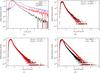Fig. 1 Histograms of the turbulent velocity fluctuations at t ≈ 0.9   s. a) Comparison between the histograms that contain the data at the flame of the resolved velocity fluctuations $\overline{\mathrm{\left|}{\mathit{v}}_{\mathrm{turb}}\mathrm{\right(}\mathit{\ell }\mathrm{\left)}\mathrm{\right|}}$ for the scales ℓ = Δ(t) and ℓ = 4Δ(t) and the histogram of the velocity fluctuations v′ [Δ(t)] of the turbulence SGS model. b) Histogram of v′(ℓcrit) using a rescaling factor of α = 1/3 (Kolmogorov) and α = 1/2 (Rayleigh-Taylor instability) using 2563 grid cells. c) Histogram of v′(ℓcrit) using a rescaling factor of α = 1/3 (Kolmogorov) and α = 1/2 (Rayleigh-Taylor instability) using 5123 grid cells. d) Comparison of the histograms of v′(ℓcrit) that contain the data at the flame front and in ash regions.

3.3.2. Rescaling of the velocity fluctuations

Since our simulation code uses a comoving grid technique, we rescale the value of v′ [Δ(t)] to v′(ℓ_crit) with ℓ_crit = 10⁶ cm (see Sect. 2). The rescaled velocity fluctuations are given by ${\mathit{v}}^{\mathrm{\prime }}\mathrm{\left(}{\mathit{\ell }}_{\mathrm{crit}}\mathrm{\right)}\mathrm{=}{\mathit{v}}^{\mathrm{\prime }}\mathrm{\left[}\mathrm{\Delta }\mathrm{\right(}\mathit{t}\mathrm{\left)}\mathrm{\right]}\mathrm{[}{\mathit{\ell }}_{\mathrm{crit}}\mathit{/}\mathrm{\Delta }\mathrm{(}\mathit{t}\mathrm{)}{\mathrm{]}}^{\mathit{\alpha }}\mathit{,}$(8)where the scaling exponent α depends on the mechanism that drives the turbulence. We assume incompressible and isotropic Kolmogorov turbulence (Kolmogorov 1941), where α = 1/3. We note, however, that Ciaraldi-Schoolmann et al. (2009) found in burned regions a transition of the turbulence-driving mechanism at a certain length scale (see also Niemeyer & Woosley 1997). This length scale is of the same order of magnitude as ℓ_crit and separates the regime of small-scale isotropic Kolmogorov turbulence from Rayleigh-Taylor instability-driven anisotropic turbulence on large scales. For the latter, α = 1/2. These considerations take into account the entire turbulent velocity field, which has well-defined statistical properties. However, for a DDT only the strong turbulent velocity fluctuations are important. Turbulence is most intense in trailing patches of the Rayleigh-Taylor “mushroom caps”, where strong shear instabilities occur (see Röpke 2007). The scaling properties of an intermittent velocity field for scales ℓ ≳ ℓ_crit in such regions at the flame front are not known. We can estimate the difference f_diff between the scaling relations of a Kolmogorov- and Rayleigh-Taylor instability-driven turbulence. Using Eq. (8), we find ${\mathit{f}}_{\mathrm{diff}}\mathrm{=}\frac{{\left[\mathrm{\Delta }\mathrm{\left(}\mathit{t}\mathrm{\right)}\mathit{/}{\mathit{\ell }}_{\mathrm{crit}}\right]}^{\mathrm{1}\mathit{/}\mathrm{2}}}{{\left[\mathrm{\Delta }\mathrm{\left(}\mathit{t}\mathrm{\right)}\mathit{/}{\mathit{\ell }}_{\mathrm{crit}}\right]}^{\mathrm{1}\mathit{/}\mathrm{3}}}\mathrm{=}{\left[\mathrm{\Delta }\mathrm{\left(}\mathit{t}\mathrm{\right)}\mathit{/}{\mathit{\ell }}_{\mathrm{crit}}\right]}^{\mathrm{1}\mathit{/}\mathrm{6}}\mathit{.}$(9)For highly resolved simulations, where Δ(t) ≈ ℓ_crit, the difference is negligible. We perform simulations with 256³ and 512³ grid cells and find for the late deflagration phase, where DDTs are expected, for the lower resolved and for the higher resolved simulation, leading to uncertainties of about 26% and 12%, respectively. To check to what extent these deviations affect the rescaled values of the high velocity fluctuations, we compare the histograms of v′(ℓ_crit) with both scaling exponents α = 1/3 and α = 1/2. Since we implement a DDT model, we now only take grid cells into account that meet certain DDT constraints; hence the data ${\mathit{N}}_{\mathrm{flame}}^{\mathrm{\ast }}\mathrm{\left(}\mathit{t}\mathrm{\right)}$ is used for the histogram construction. The result is shown in Fig. 1b,c for the late deflagration phase at . The agreement of both histograms is excellent, particularly in the high resolution case.

We note that intermittency may slow down the decrease of the velocity fluctuations towards smaller scales, compared to the scaling given in Eq. (8). However, if it dominates the scaling behavior, it may change the trend completely. Our model would still be a good approximation in the first case. Comparing the histograms in Fig. 1a suggests that the velocity fluctuations indeed still decrease with scale, but a more rigorous verification is not possible with our simulations. While studying intermittency effects in ash regions is possible based on the computation of structure functions of the velocity field (Schmidt et al. 2010; Ciaraldi-Schoolmann et al. 2009), such functions cannot easily be determined at the flame front itself for geometrical reasons.

3.3.3. Fitting the data of the histogram

To calculate the probability of finding sufficiently high velocity fluctuations for a DDT, we apply a fit to the histogram of v′(ℓ_crit) to obtain an approximated PDF (see also Röpke 2007). Since for a DDT only the high velocity fluctuations are of interest, we are justified in restricting our fit to the right of the maximum of the histogram. The fit should further be motivated by an appropriate distribution function that can explain the intermittent behavior in turbulence at the flame. Schmidt et al. (2010) used a log-normal distribution of an intermittency model of Kolmogorov (1962) and Oboukhov (1962) to fit characteristic scaling exponents that were obtained from the computation of high-order velocity correlation functions. This detailed analysis revealed that the intermittency in ash regions is weaker than predicted in the log-normal model. In contrast, Röpke (2007) found that a log-normal fit fails to reproduce the distribution of the high velocity fluctuations at the flame since it declines faster toward larger v′(ℓ_crit) than do the velocity data of the histogram. This result suggests that intermittency at the flame is fundamentally different than in ash (see also the discussion in Schmidt et al. 2010). In Fig. 1d we show histograms of v′(ℓ_crit) that contain the data ${\mathit{N}}_{\mathrm{flame}}^{\mathrm{\ast }}\mathrm{\left(}\mathit{t}\mathrm{\right)}$ and the data in ash regions in the late deflagration phase at t ≈ 0.9 s (again, this instant is chosen as an illustrative example). The simulation was run with 512³ grid cells. There is a significant difference between the shapes of the PDFs. The slow decline of the histogram that contains the data in ash regions appears almost linear in the log-normal illustration, while the histogram that contains the data in the vicinity of the flame has a significant positive curvature after its maximum. This is further evidence that turbulence near the flame has stronger intermittency than in ash regions.

As of yet there is no physically motivated model for explaining intermittency at a deflagration front in white dwarfs. Consequently, an empirical distribution function has to be used to fit the slow decline of the histogram of v′(ℓ_crit) at the flame front. Here we follow Röpke (2007) and use an ansatz of the form $\mathit{f}\mathrm{\left[}{\mathit{v}}^{\mathrm{\prime }}\mathrm{\right(}{\mathit{\ell }}_{\mathrm{crit}}\mathrm{\left)}\mathrm{\right]}\mathrm{=}\exp \mathrm{\left\{}{\mathit{a}}_{\mathrm{1}}\mathrm{\right[}{\mathit{v}}^{\mathrm{\prime }}\mathrm{\left(}{\mathit{\ell }}_{\mathrm{crit}}\mathrm{\right)}{\mathrm{]}}^{{\mathit{a}}_{\mathrm{2}}}\mathrm{+}{\mathit{a}}_{\mathrm{3}}\mathrm{\}}\mathit{.}$(10)This geometric function is able to fit the right part of the histogram over a large range and a₁, a₂ and a₃ are the three fitting parameters. The probability $\mathit{P}\mathrm{\left[}{\mathit{v}}^{\mathrm{\prime }}\mathrm{\right(}{\mathit{\ell }}_{\mathrm{crit}}\mathrm{)}\mathrm{\ge }{\mathit{v}}_{\mathrm{crit}}^{\mathrm{\prime }}\mathrm{]}\mathrm{\left(}\mathit{t}\mathrm{\right)}$ of finding velocity fluctuations of at least ${\mathit{v}}_{\mathrm{crit}}^{\mathrm{\prime }}$ is given by $\begin{array}{ccc}\mathit{P}\mathrm{\left[}{\mathit{v}}^{\mathrm{\prime }}\mathrm{\right(}{\mathit{\ell }}_{\mathrm{crit}}\mathrm{)}\mathrm{\ge }{\mathit{v}}_{\mathrm{crit}}^{\mathrm{\prime }}\mathrm{]}\mathrm{\left(}\mathit{t}\mathrm{\right)}\mathrm{=}{\mathrm{\int }}_{{\mathit{v}}_{\mathrm{crit}}^{\mathrm{\prime }}}^{\mathrm{\infty }}\mathit{f}\mathrm{\left[}{\mathit{v}}^{\mathrm{\prime }}\mathrm{\right(}{\mathit{\ell }}_{\mathrm{crit}}\mathrm{\left)}\mathrm{\right]}\mathrm{d}{\mathit{v}}^{\mathrm{\prime }}\mathrm{\left(}{\mathit{\ell }}_{\mathrm{crit}}\mathrm{\right)}& & \\ \mathrm{=}\frac{\exp \mathrm{\left(}{\mathit{a}}_{\mathrm{3}}\mathrm{\right)}\mathrm{\Gamma }\mathrm{(}\mathrm{1}\mathit{/}{\mathit{a}}_{\mathrm{2}}\mathit{,}\mathrm{-}{\mathit{a}}_{\mathrm{1}}{\mathit{v}}^{{\mathit{a}}_{\mathrm{2}}}\mathrm{)}}{{\mathit{a}}_{\mathrm{2}}\mathrm{(}\mathrm{-}{\mathit{a}}_{\mathrm{1}}{\mathrm{)}}^{\mathrm{1}\mathit{/}{\mathit{a}}_{\mathrm{2}}}}\mathit{,}& & \end{array}$(11)where Γ is the upper incomplete gamma function.

We note that the DDT instant determined below is not really a special point in the time evolution of the PDF. When a detonation is triggered in the model, the parts of the deflagration flame that are directly attached to the quickly spreading detonation front are excluded from the determination of the PDF.

3.4. The detonation area and the DDT criterion

In Sect. 3.2 we defined ${\mathit{A}}_{\mathrm{flame}}^{\mathrm{\ast }}\mathrm{\left(}\mathit{t}\mathrm{\right)}$ as the part of the flame that meets the required conditions for a DDT concerning the quantities ρ_fuel and X_fuel. The probability of finding sufficiently high velocity fluctuations at this restricted flame surface area was derived separately in the previous section. We define now ${\mathit{A}}_{\det }\mathrm{\left(}\mathit{t}\mathrm{\right)}\mathrm{=}{\mathit{A}}_{\mathrm{flame}}^{\mathrm{\ast }}\mathrm{\left(}\mathit{t}\mathrm{\right)}\mathit{P}\mathrm{\left[}{\mathit{v}}^{\mathrm{\prime }}\mathrm{\right(}{\mathit{\ell }}_{\mathrm{crit}}\mathrm{)}\mathrm{\ge }{\mathit{v}}_{\mathrm{crit}}^{\mathrm{\prime }}\mathrm{]}\mathrm{\left(}\mathit{t}\mathrm{\right)}$(12)as the part of the flame surface area that can potentially undergo a DDT (see also Röpke 2007). This quantity has to exceed a critical value A_crit, which is required for a DDT. We assume that a DDT region has a smooth two-dimensional geometry and use therefore . For A_det(t) > A_crit, we finally check whether this condition holds for at least τ_eddy1/2(ℓ_crit) to ensure a sufficient mixing (see Sect. 2). If this is true, our DDT criterion is met and detonations are initialized. 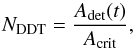The number of DDTs N_DDT in our model is given by ${\mathit{N}}_{\mathrm{DDT}}\mathrm{=}\frac{{\mathit{A}}_{\det }\mathrm{\left(}\mathit{t}\mathrm{\right)}}{{\mathit{A}}_{\mathrm{crit}}}\mathit{,}$(13)where N_DDT is always rounded down to the next integer. We note that both quantities ${\mathit{A}}_{\mathrm{flame}}^{\mathrm{\ast }}\mathrm{\left(}\mathit{t}\mathrm{\right)}$ and particularly may rise steeply within τ_eddy1/2(ℓ_crit); hence we often get N_DDT > 1. The minimum time between two DDTs is τ_eddy1/2(ℓ_crit), because the time for A_det(t) > A_crit is restarted after a successful DDT. It is also restarted if A_det(t) falls below A_crit before τ_eddy1/2(ℓ_crit) is reached.

We still have to decide on the location where detonations are initialized. Since the high turbulent velocity fluctuations are crucial for a DDT, we chose those N_DDT grid cells from ${\mathit{N}}_{\mathrm{flame}}^{\mathrm{\ast }}\mathrm{\left(}\mathit{t}\mathrm{\right)}$ that contain the highest values of v′(ℓ_crit). In analogy to the deflagration ignition, detonations are set by initializing an additional level set that propagates supersonically at the appropriate detonation speed (see Fink et al. 2010) through the white dwarf matter.

A shortcoming of this DDT model is that it does not assess whether there is indeed a “connected” region of size that fulfills the requirements for a DDT. The probability $\mathit{P}\mathrm{\left[}{\mathit{v}}^{\mathrm{\prime }}\mathrm{\right(}{\mathit{\ell }}_{\mathrm{crit}}\mathrm{)}\mathrm{\ge }{\mathit{v}}_{\mathrm{crit}}^{\mathrm{\prime }}\mathrm{]}\mathrm{\left(}\mathit{t}\mathrm{\right)}$ and the flame surface area ${\mathit{A}}_{\mathrm{flame}}^{\mathrm{\ast }}\mathrm{\left(}\mathit{t}\mathrm{\right)}$ are determined from all (possibly disconnected) grid cells suitable for a DDT. Therefore they do not provide any information on localized areas. They are rather global quantities. The same holds for τ_eddy1/2(ℓ_crit) since here we also use a uniform value.

From a computational point of view, we emphasize that the inclusion of τ_eddy1/2(ℓ_crit) is also important to keep the DDT criterion independent of resolution. Since the maximum time step Δ_CFL of our code is given by the Courant-Friedrichs-Lewy (CFL) condition (Courant & Friedrichs 1948), the time steps of higher resolved simulations are shorter than for lower resolved ones. Applying our criterion without a time-dependent variable would mean that higher resolved simulations get an enhanced chance for a successful detonation. This simply results from the fact that the criterion then tests for DDTs more frequently. We note that in our simulations Δ_CFL is usually much shorter than τ_eddy1/2(ℓ_crit).

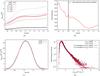Fig. 2 Analysis of the fractal dimension of the flame and resolution dependence of the histogram of v′(ℓcrit). a) Number of all grid cells at the flame front for two different resolutions (thick curves) as well as theoretical curves if a specific fractal dimension is assumed. b) Fractal dimension D of the flame as function of time. c) Flame surface area ${\mathit{A}}_{\mathrm{flame}}^{\mathrm{\ast }}\mathrm{\left(}\mathit{t}\mathrm{\right)}$ for different resolutions with D = 2.36. d) Histograms of v′(ℓcrit) at the flame front and the corresponding fits (Eq. (10)) for different resolutions.

4. Fractal dimension of the flame and resolution test in one full-star model

To test the resolution dependence of the implemented DDT criterion, we apply it to the deflagration model described in Sect. 3.1 and run it with a resolution of 256³ and 512³ grid cells. Unfortunately, we cannot perform a detailed resolution study since simulations with more than 512³ grid cells are computationally too expensive, while the DDT model cannot be applied for very low resolved simulations due to insufficient data for fitting the histogram of v′(ℓ_crit). In summary, the quantities and the corresponding threshold values of the DDT criterion are 1/3 ≤ X_fuel ≤ 2/3, 0.5 ≲ ρ_fuel/(10⁷   g  cm^-3) ≲ 1.5, , , and . One parameter still undetermined is the fractal dimension of the flame, which we now derive from the resolution test.

4.1. Fractal dimension of the flame

In Fig. 2a we show N_flame(t). The thick black curve is the result for the lower resolved simulation and the thick red (dashed) curve for the higher resolved one. The other curves are theoretically expected results for the higher resolved simulation if a certain fractal dimension of the flame is assumed. These curves can be calculated from N_flame1(t) and the known resolutions Δ₁(t) and Δ₂(t) of the simulations by specifying a value for D in Eq. (5). We see that the curves for D = 2 and D = 3 are not consistent with the data, which shows that the flame is indeed a fractal.

In Fig. 2b the fractal dimension D (calculated from Eq. (4) is shown as function of time. A necessary constraint in our criterion is that ρ_fuel must be in a certain range (see Sect. 2). At approximately , the first grid cells at the flame front approach , while most of the flame resides at higher densities. We see that at this time D ≈ 2.5, but DDTs will occur later when a sufficiently large part of the flame surface area meets the DDT constraints and τ_eddy1/2(ℓ_crit) has elapsed. At these times, D < 2.5. In agreement with theory (e.g., Halsey et al. 1986; Sreenivasan 1991), we use a constant value of D = 2.36 for our DDT model (see Sect. 3.2). In Fig. 2c, we show the quantity ${\mathit{A}}_{\mathrm{flame}}^{\mathrm{\ast }}\mathrm{\left(}\mathit{t}\mathrm{\right)}$ (calculated from Eq. (6) with D = 2.36) for both simulations. Since the curves are in good agreement, the choice of D = 2.36 is justified.

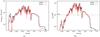Fig. 3 a) Probability of finding velocity fluctuations higher than and b) size of the potential detonation area Adet(t). For most of the time between and , Adet(t) > Acrit holds. The DDT criterion is met for the first time at in both simulations (see dots at the curve of Adet(t)).

We next discuss some caveats concerning the determination of the fractal dimension of the flame. It is obviously a rough approximation to take D as a constant since we see in Fig. 2b that this quantity declines continuously until t ≈ 1.2 s. Moreover, one could expect that models with a different deflagration phase may have another curve progression of D. Therefore a determination of D for every delayed detonation simulation that has a different evolution of the deflagration would be necessary. However, at the time when DDTs occur, we assume that turbulence in the deflagration phase is fully developed and obeys well-defined statistical properties. Hence a significant deviation of D for different deflagrations seems unlikely but cannot be ruled out completely. Finally, the results may be different if higher resolutions with more data are used for the determination of D, so that a convergence of D may be obtained at very high resolutions only. Apart from the limited computational resources that prevent simulations at such high resolutions, we mention in Sect. 3.2 that the flame is not an ideal fractal, so that at some length scale Eq. (4) becomes inappropriate to derive D.

We note that the values for D in Fig. 2b may also indicate that the flame is affected by different mechanisms and instabilities that drive the turbulence because 2.3 ≲ D ≲ 2.5 are expected for different instabilities at the flame front (see Sect. 3.2). In any case, the chosen value of D = 2.36 is appropriate for our purposes since both curves of ${\mathit{A}}_{\mathrm{flame}}^{\mathrm{\ast }}\mathrm{\left(}\mathit{t}\mathrm{\right)}$ in Fig. 2c are in good agreement.

4.2. Probability of finding high velocity fluctuations

In Fig. 2d, a histogram of v′(ℓ_crit) with the fit according to Eq. (10) through the data for both simulations is shown at . Since we are mainly interested in the high velocity fluctuations, the starting point of the fit is at twice the velocity at the maximum of the corresponding histogram. We see that the approximated PDFs are in very good agreement with the histograms. For the lower resolved simulation, however, the data contain more scatter and there is an earlier cutoff toward higher velocity fluctuations. This is the result of a coarser binning due to less data in lower resolved simulations.

The probability is shown in Fig. 3a for both simulations. The good agreement of both curves reflects that the approximated PDFs are largely independent of resolution. The highest values are found for when the intermittency in the turbulence is most pronounced.

4.3. Detonation area

The quantity A_det(t) is shown in Fig. 3b for both resolutions. Since A_det(t) is calculated from ${\mathit{A}}_{\mathrm{flame}}^{\mathrm{\ast }}\mathrm{\left(}\mathit{t}\mathrm{\right)}$ and , it is also independent of resolution. This manifests in Fig. 3, in which the overall shape of the curve of A_det(t) is very similar to that of . In particular the strong variations of can be identified again. This indicates that the change of the flame surface area ${\mathit{A}}_{\mathrm{flame}}^{\mathrm{\ast }}\mathrm{\left(}\mathit{t}\mathrm{\right)}$ for a given interesting time interval τ_eddy1/2(ℓ_crit) is much smaller than the fast temporal variations of the probability . To see this, compare ${\mathit{A}}_{\mathrm{flame}}^{\mathrm{\ast }}\mathrm{\left(}\mathit{t}\mathrm{\right)}$ in Fig. 2c with Fig. 3a.

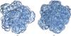Fig. 4 Deflagration flame (transparent iso-surface) at the time of the first DDT for both simulations. The DDT spots are encircled. a) Simulation with 2563 grid cells. b) Simulation with 5123 grid cells.

For our resolution test, we have chosen , and we see that this value is exceeded by A_det(t). Therefore, DDTs will occur if A_det(t) > A_crit for at least τ_eddy1/2(ℓ_crit). This condition is indeed reached in both simulations, where the first DDTs are initialized at approximately . This time is marked with a dot at the curve of A_det in Fig. 3b. For the lower resolved simulation, we find A_det ≈ 1.72 × 10¹²; hence N_DDT = 1. In the higher resolved simulation we find A_det ≈ 2.12 × 10¹²; hence here detonations are already initialized in two grid cells. We note that these cells are located at different deflagration plumes and are spatially disconnected. As long as A_det(t) > A_crit for τ_eddy1/2(ℓ_crit), new DDTs commence at later time steps. This happens in our simulations since A_det(t) > A_crit for most of the time in the interval 0.92   s ≲ t ≲ 1.07   s. However, there are a few interruptions: In some time steps, the condition A_det(t) < A_crit occurs before τ_eddy1/2(ℓ_crit) was reached, preventing some DDTs. The maximum of N_DDT is 10 for the lower resolved and 12 for the higher resolved simulation, which is reached at for both cases. The last DDT occurs at in one single grid cell in both simulations.

In Fig. 4, the time of the first DDT is visualized for both simulations. The deflagration flame, represented by the level set function, is shown as a transparent iso-surface. While the number of DDTs is largely resolution independent, their localization is generally quite different. In Fig. 4, the first DDT occurs at different places at the deflagration flame (both figures show the same viewing angle). The reason is that the exact number and locations of the grid cells in which the highest velocity fluctuations occur differs. In subsequent papers in this series, we will show that different distributions of DDT spots have an impact on the ⁵⁶Ni production rate in the detonation phase.

5. Conclusion

We introduced the first subgrid-scale model for implementing DDTs in a hydrodynamic code for large-scale simulations of SN Ia explosions. The model includes the current knowledge on DDTs in SNe Ia and can be summarized as follows: We first ensure that a sufficient number of grid cells at the flame have a certain fuel fraction and are in a certain fuel density range. From the number and size of these cells, we determine a suitable flame surface area for DDTs, where we assume that the flame can be considered as a fractal. Simultaneously, we construct a histogram of the turbulent velocity fluctuations in the above-mentioned cells, where we rescale these fluctuations from the grid scale to the critical length scale of a DDT region by assuming Kolmogorov turbulence. Then we estimate the probability of finding sufficiently high velocity fluctuations for a DDT by applying a fit function to the histogram. This probability multiplied by the flame surface area that is suitable for a DDT constitutes a potential detonation area, which we compare with the required critical size of a DDT region. When the potential detonation area exceeds this critical size for at least half of an eddy turnover time, the DDT constraints are fulfilled. In this case detonations are initialized in the grid cells with the highest velocity fluctuations that are located within the flame surface area suitable for a DDT. The number of initialized detonations equals the ratio of the potential detonation area to the critical size of a DDT region.

Although our model refers to the initiation of the detonation via the Zel’dovich gradient mechanism, we note that other proposed mechanisms for forming a detonation out of a turbulent deflagration burning regime (Poludnenko et al. 2011; Kushnir et al. 2012) would require a similar parameterization of the DDT-SGS model. In all cases, the critical quantity is the strength of turbulence. However, the models of Poludnenko et al. (2011) and Kushnir et al. (2012) require turbulence speeds close to sonic, which we do not observe in our simulations of deflagrations in white dwarfs. The velocity fluctuations of 10⁸   cm   s^-1 assumed in our DDT-SGS model correspond to Mach numbers of ~0.3 with respect to the fuel material (~0.1 with respect to the ashes) in the density range in which DDTs are expected.

We show that the DDT-SGS model is largely resolution independent. Assuming that the DDT region has a smooth two-dimensional geometry we found that the criterion is met in a specific deflagration model, indicating that the necessary constraints for DDTs in SNe Ia were appropriate. Our model includes a global criterion because the histograms of v′(ℓ_crit) and ${\mathit{A}}_{\mathrm{flame}}^{\mathrm{\ast }}\mathrm{\left(}\mathit{t}\mathrm{\right)}$ do not provide any information about local areas. Therefore, a shortcoming of our model is that we cannot fully ensure that there is indeed a compact region that obeys the necessary constraints for a DDT.

For testing our DDT model, we used a specific simulation of the deflagration phase in a thermonuclear explosion of a Chandrasekhar-mass WD. The evolution of the turbulent deflagration depends strongly on the ignition scenario of the flame, which is currently unknown. Certain turbulent deflagrations will meet a given DDT criterion more frequently, which will consequently affect the occurrence of DDTs. Therefore the ignition scenario of the deflagration is another crucial model parameter for simulations of delayed detonations. An analysis of the importance of the ignition scenario for the DDT-SGS model will be the subject of future research. The values of the DDT parameters are not well known and have been kept constant or fixed in a certain range in our DDT model. For this reason, we intend to perform a parameter study by varying all DDT quantities. These future studies will reveal further insights into the relevance and constraints of delayed detonations in Chandrasekhar-mass white dwarfs.

Acknowledgments

This work was partially supported by the Deutsche Forschungsgemeinschaft via the Transregional Collaborative Research Center TRR 33 “The Dark Universe”, the Excellence Cluster EXC153 “Origin and Structure of the Universe”, the Emmy Noether Program (RO 3676/1-1), and the graduate school “Theoretical Astrophysics and Particle Physics” GRK 1147. FKR also acknowledges financial support by the ARCHES prize of the German Ministry of Education and Research (BMBF) and by the Group of Eight/Deutscher Akademischer Austausch Dienst (Go8/DAAD) German-Australian exchange program.

References

All Figures

Fig. 1 Histograms of the turbulent velocity fluctuations at t ≈ 0.9   s. a) Comparison between the histograms that contain the data at the flame of the resolved velocity fluctuations $\overline{\mathrm{\left|}{\mathit{v}}_{\mathrm{turb}}\mathrm{\right(}\mathit{\ell }\mathrm{\left)}\mathrm{\right|}}$ for the scales ℓ = Δ(t) and ℓ = 4Δ(t) and the histogram of the velocity fluctuations v′ [Δ(t)] of the turbulence SGS model. b) Histogram of v′(ℓcrit) using a rescaling factor of α = 1/3 (Kolmogorov) and α = 1/2 (Rayleigh-Taylor instability) using 2563 grid cells. c) Histogram of v′(ℓcrit) using a rescaling factor of α = 1/3 (Kolmogorov) and α = 1/2 (Rayleigh-Taylor instability) using 5123 grid cells. d) Comparison of the histograms of v′(ℓcrit) that contain the data at the flame front and in ash regions.

In the text

Fig. 2 Analysis of the fractal dimension of the flame and resolution dependence of the histogram of v′(ℓcrit). a) Number of all grid cells at the flame front for two different resolutions (thick curves) as well as theoretical curves if a specific fractal dimension is assumed. b) Fractal dimension D of the flame as function of time. c) Flame surface area ${\mathit{A}}_{\mathrm{flame}}^{\mathrm{\ast }}\mathrm{\left(}\mathit{t}\mathrm{\right)}$ for different resolutions with D = 2.36. d) Histograms of v′(ℓcrit) at the flame front and the corresponding fits (Eq. (10)) for different resolutions.

In the text

	Fig. 3 a) Probability of finding velocity fluctuations higher than and b) size of the potential detonation area Adet(t). For most of the time between and , Adet(t) > Acrit holds. The DDT criterion is met for the first time at in both simulations (see dots at the curve of Adet(t)).
In the text

	Fig. 4 Deflagration flame (transparent iso-surface) at the time of the first DDT for both simulations. The DDT spots are encircled. a) Simulation with 2563 grid cells. b) Simulation with 5123 grid cells.
In the text

References

- Arnett, D., & Livne, E. 1994, ApJ, 427, 330 [NASA ADS] [CrossRef] [Google Scholar]
- Arnett, W. D., Truran, J. W., & Woosley, S. E. 1971, ApJ, 165, 87 [NASA ADS] [CrossRef] [Google Scholar]
- Aspden, A. J., Bell, J. B., Day, M. S., Woosley, S. E., & Zingale, M. 2008, ApJ, 689, 1173 [NASA ADS] [CrossRef] [Google Scholar]
- Blinnikov, S. I., & Khokhlov, A. M. 1986, Sov. Astron. Lett., 12, 131 [NASA ADS] [Google Scholar]
- Blinnikov, S. I., & Khokhlov, A. M. 1987, Sov. Astron. Lett., 13, 364 [NASA ADS] [Google Scholar]
- Blinnikov, S. I., & Sasorov, P. V. 1996, Phys. Rev. E, 53, 4827 [NASA ADS] [CrossRef] [Google Scholar]
- Charignon, C., & Chièze, J.-P. 2013, A&A, 550, A105 [NASA ADS] [CrossRef] [EDP Sciences] [Google Scholar]
- Ciaraldi-Schoolmann, F., Schmidt, W., Niemeyer, J. C., Röpke, F. K., & Hillebrandt, W. 2009, ApJ, 696, 1491 [NASA ADS] [CrossRef] [Google Scholar]
- Colella, P., & Woodward, P. R. 1984, J. Comput. Phys., 54, 174 [NASA ADS] [CrossRef] [MathSciNet] [Google Scholar]
- Colgate, S. A., & McKee, C. 1969, ApJ, 157, 623 [NASA ADS] [CrossRef] [Google Scholar]
- Contardo, G., Leibundgut, B., & Vacca, W. D. 2000, A&A, 359, 876 [NASA ADS] [Google Scholar]
- Courant, R., & Friedrichs, K. O. 1948, Supersonic Flow and Shock Waves (New York: Springer Verlag) [Google Scholar]
- Dursi, L. J., & Timmes, F. X. 2006, ApJ, 641, 1071 [NASA ADS] [CrossRef] [Google Scholar]
- Fink, M., Röpke, F. K., Hillebrandt, W., et al. 2010, A&A, 514, A53 [NASA ADS] [CrossRef] [EDP Sciences] [Google Scholar]
- Fryxell, B. A., Müller, E., & Arnett, W. D. 1989, Hydrodynamics and nuclear burning, MPA Green Report 449, Max-Planck-Institut für Astrophysik, Garching [Google Scholar]
- Gamezo, V. N., Khokhlov, A. M., Oran, E. S., Chtchelkanova, A. Y., & Rosenberg, R. O. 2003, Science, 299, 77 [NASA ADS] [CrossRef] [PubMed] [Google Scholar]
- Gamezo, V. N., Khokhlov, A. M., & Oran, E. S. 2005, ApJ, 623, 337 [NASA ADS] [CrossRef] [Google Scholar]
- Golombek, I., & Niemeyer, J. C. 2005, A&A, 438, 611 [NASA ADS] [CrossRef] [EDP Sciences] [Google Scholar]
- Halsey, T. C., Jensen, M. H., Kadanoff, L. P., Procaccia, I., & Shraiman, B. I. 1986, Phys. Rev. A, 33, 1141 [NASA ADS] [CrossRef] [MathSciNet] [PubMed] [Google Scholar]
- Hillebrandt, W., & Niemeyer, J. C. 2000, ARA&A, 38, 191 [NASA ADS] [CrossRef] [Google Scholar]
- Höflich, P., Wheeler, J. C., & Thielemann, F. K. 1998, ApJ, 495, 617 [NASA ADS] [CrossRef] [Google Scholar]
- Jackson, A. P., Calder, A. C., Townsley, D. M., et al. 2010, ApJ, 720, 99 [NASA ADS] [CrossRef] [Google Scholar]
- Kasen, D., Röpke, F. K., & Woosley, S. E. 2009, Nature, 460, 869 [NASA ADS] [CrossRef] [Google Scholar]
- Kerstein, A. R. 1988, Combust. Sci. Technol., 60, 441 [CrossRef] [Google Scholar]
- Kerstein, A. R. 1991, Phys. Rev. A, 44, 3633 [NASA ADS] [CrossRef] [Google Scholar]
- Kerstein, A. R. 2001, Phys. Rev. E, 64, 066306 [NASA ADS] [CrossRef] [Google Scholar]
- Khokhlov, A. M. 1991a, A&A, 245, 114 [NASA ADS] [Google Scholar]
- Khokhlov, A. M. 1991b, A&A, 246, 383 [NASA ADS] [Google Scholar]
- Khokhlov, A. M. 1995, ApJ, 449, 695 [NASA ADS] [CrossRef] [Google Scholar]
- Khokhlov, A. M. 2000 [arXiv:astro-ph/0008463] [Google Scholar]
- Khokhlov, A. M., Oran, E. S., & Wheeler, J. C. 1997, ApJ, 478, 678 [NASA ADS] [CrossRef] [Google Scholar]
- Kolmogorov, A. N. 1941, Dokl. Akad. Nauk SSSR, 30, 299, in Russian [Google Scholar]
- Kolmogorov, A. N. 1962, J. Fluid Mech., 13, 82 [NASA ADS] [CrossRef] [Google Scholar]
- Kozma, C., Fransson, C., Hillebrandt, W., et al. 2005, A&A, 437, 983 [Google Scholar]
- Kushnir, D., Livne, E., & Waxman, E. 2012, ApJ, 752, 89 [NASA ADS] [CrossRef] [Google Scholar]
- Lisewski, A. M., Hillebrandt, W., & Woosley, S. E. 2000, ApJ, 538, 831 [NASA ADS] [CrossRef] [Google Scholar]
- Mazzali, P. A., Röpke, F. K., Benetti, S., & Hillebrandt, W. 2007, Science, 315, 825 [NASA ADS] [CrossRef] [PubMed] [Google Scholar]
- Niemeyer, J. C. 1995, Ph.D. thesis, Technical University of Munich, also available as MPA Green Report 911 [Google Scholar]
- Niemeyer, J. C., & Woosley, S. E. 1997, ApJ, 475, 740 [NASA ADS] [CrossRef] [Google Scholar]
- Oboukhov, A. M. 1962, J. Fluid Mech., 13, 77 [NASA ADS] [CrossRef] [MathSciNet] [Google Scholar]
- Peters, N. 2000, Turbulent Combustion (Cambridge: Cambridge University Press) [Google Scholar]
- Poludnenko, A. Y., Gardiner, T. A., & Oran, E. S. 2011, Phys. Rev. Lett., 107, 054501 [NASA ADS] [CrossRef] [PubMed] [Google Scholar]
- Reinecke, M., Hillebrandt, W., Niemeyer, J. C., Klein, R., & Gröbl, A. 1999, A&A, 347, 724 [NASA ADS] [Google Scholar]
- Röpke, F. K. 2005, A&A, 432, 969 [NASA ADS] [CrossRef] [EDP Sciences] [Google Scholar]
- Röpke, F. K. 2007, ApJ, 668, 1103 [NASA ADS] [CrossRef] [Google Scholar]
- Röpke, F. K., & Niemeyer, J. C. 2007, A&A, 464, 683 [NASA ADS] [CrossRef] [EDP Sciences] [Google Scholar]
- Röpke, F. K., Hillebrandt, W., Niemeyer, J. C., & Woosley, S. E. 2006, A&A, 448, 1 [NASA ADS] [CrossRef] [EDP Sciences] [Google Scholar]
- Röpke, F. K., Hillebrandt, W., Schmidt, W., et al. 2007, ApJ, 668, 1132 [NASA ADS] [CrossRef] [Google Scholar]
- Röpke, F. K., Kromer, M., Seitenzahl, I. R., et al. 2012, ApJ, 750, L19 [NASA ADS] [CrossRef] [Google Scholar]
- Schmidt, W. 2007, A&A, 465, 263 [NASA ADS] [CrossRef] [EDP Sciences] [Google Scholar]
- Schmidt, W., Niemeyer, J. C., & Hillebrandt, W. 2006a, A&A, 450, 265 [NASA ADS] [CrossRef] [EDP Sciences] [Google Scholar]
- Schmidt, W., Niemeyer, J. C., Hillebrandt, W., & Röpke, F. K. 2006b, A&A, 450, 283 [NASA ADS] [CrossRef] [EDP Sciences] [Google Scholar]
- Schmidt, W., Ciaraldi-Schoolmann, F., Niemeyer, J. C., Röpke, F. K., & Hillebrandt, W. 2010, ApJ, 710, 1683 [NASA ADS] [CrossRef] [Google Scholar]
- Seitenzahl, I. R., Meakin, C. A., Townsley, D. M., Lamb, D. Q., & Truran, J. W. 2009, ApJ, 696, 515 [NASA ADS] [CrossRef] [Google Scholar]
- Seitenzahl, I. R., Ciaraldi-Schoolmann, F., & Röpke, F. K. 2011, MNRAS, 414, 2709 [NASA ADS] [CrossRef] [Google Scholar]
- Seitenzahl, I. R., Ciaraldi-Schoolmann, F., Röpke, F. K., et al. 2013, MNRAS, 429, 1156 [Google Scholar]
- Sreenivasan, K. R. 1991, Ann. Rev. Fluid Mech., 23, 539 [Google Scholar]
- Stritzinger, M., Leibundgut, B., Walch, S., & Contardo, G. 2006, A&A, 450, 241 [NASA ADS] [CrossRef] [EDP Sciences] [Google Scholar]
- Townsley, D. M., Jackson, A. P., Calder, A. C., et al. 2009, ApJ, 701, 1582 [NASA ADS] [CrossRef] [Google Scholar]
- Truran, J. W., Arnett, W. D., & Cameron, A. G. W. 1967, Can. J. Phys., 45, 2315 [NASA ADS] [CrossRef] [Google Scholar]
- Woosley, S. E. 2007, ApJ, 668, 1109 [NASA ADS] [CrossRef] [Google Scholar]
- Woosley, S. E., Kerstein, A. R., Sankaran, V., Aspden, A. J., & Röpke, F. K. 2009, ApJ, 704, 255 [NASA ADS] [CrossRef] [Google Scholar]
- Zel’dovich, Y. B., Librovich, V. B., Makhviladze, G. M., & Sivashinskii, G. I. 1970, J. Appl. Mech. Tech. Phys., 11, 264 [NASA ADS] [CrossRef] [Google Scholar]