| Issue |
A&A
Volume 558, October 2013
|
|
|---|---|---|
| Article Number | A138 | |
| Number of page(s) | 10 | |
| Section | Astronomical instrumentation | |
| DOI | https://doi.org/10.1051/0004-6361/201322304 | |
| Published online | 22 October 2013 | |
Theoretical performance of solar coronagraphs using sharp-edged or apodized circular external occulters
Université de Nice Sophia-Antipolis, Centre National de la Recherche
Scientifique, Observatoire de la Côte d’Azur, UMR7293 Lagrange,
Parc Valrose,
06108
Nice,
France
e-mail:
claude.aime@unice.fr
Received:
17
July
2013
Accepted:
4
September
2013
Context. This study focuses on an instrument able to monitor the corona close to the solar limb.
Aims. We study the performance of externally occulted solar coronagraphs. We compute the shape of the umbra and penumbra produced by the occulter at the entrance aperture of the telescope and compare levels of rejection obtained for a circular occulter with a sharp or smooth transmission at the edge.
Methods. We show that the umbral pattern in an externally occulted coronagraph can be written as a convolution product between the occulter diffraction pattern and an image of the Sun. We then focus on the analysis to circular symmetric occulters. We first derive an analytical expression using two Lommel series for the Fresnel diffraction pattern produced by a sharp-edged circular occulter. Two different expressions are used for inside and outside the occulter’s geometric shadow. We verify that a numerical approach that directly solves the Huygens-Fresnel integral gives the same result. This suggests that the numerical computation can be used for a circular occulter with any variable transmission.
Results. With the objective of observing the solar corona a few minutes from limb, a sharp-edged circular occulter of a few meters cannot produce an umbra darker than 10-4 of the direct sunlight. The same occulter, having an apodization zone of a few percent of the diameter (3 cm for a 1.5 m occulter), darkers the umbra down to 10-8 of the direct sunlight for linear transmission and to 10-12 for Sonine or cosine bell transmissions. An investigation for an apodized occulter with manufacturing defaults is quickly performed.
Conclusions. It has been possible to numerically demonstrate the large superiority of apodized circular occulters with respect to the sharp-edged ones. These occulters allow the theoretical observation of the very limb-close corona with not yet obtained contrast ratios.
Key words: Sun: corona / instrumentation: high angular resolution / methods: analytical
© ESO, 2013
1. Introduction
The observation of the solar corona in absence of total solar eclipses was first realized with the historical experiment of Lyot (1939). The concept of a coronagraph with an external occulter was proposed by Evans (1948), and the use of sawtooth disk occulters were considered by Purcell & Koomen (1962). An excellent description of the methods based on external occulters of various kinds (simple, shaped, or multiple) can be found in the review paper by Koutchmy (1988). Here, we only consider a single circular occulter with either a sharp-edge or a variable transmission at the edge.
External occulters using flying spacecrafts were envisaged for the direct detection of exoplanets by Marchal (1985), and several projects, such as those of Cash (2006) or Vanderbei et al. (2007), have considered the use of petal-shaped occulters. Due to respective constraints, the geometry of the solar and stellar experiments are entirely different. For exoplanets, giant occulters of the order of 50 m at 100 000 km are needed to produce umbras deeper than 10-10 of the direct starlight over the entrance aperture of a 4-m telescope. The envisaged obscuration angle is of the order of 0.1 arc sec or smaller, which is the angular separation to achieve for a Sun-Earth system at a distance of 10 parsec.
For the solar corona, the entire solar disc of 32 arc minutes must be obscured by the occulter, and the level of the residual light must be less than 10-6 of the photospheric intensity. The observation must be possible as close as a few arc minutes to the solar limb. The project ASPIICS (Association de Satellites Pour l’Imagerie et l’Interférométrie de la Couronne Solaire) described by Lamy et al. (2010) and Vives et al. (2009) envisages the use of occulters in the meter range (1.5 m) and the observing telescope of a few centimeters, whose distance is roughly 100 times the occulter diameter. We expect to observe the low solar corona at a much closer distance to the limb than what was determined with the LASCO (Large Angle Spectroscopic Coronagraph) experiment described in Brueckner et al. (1995).
A study of performance of the ASPIICS project that considers diffraction effects was already made by Verroi et al. (2008). They concluded that a sharp-edged circular occulter was not able to reach the desired rejection, a performance that can be obtained with serrated-edge occulters. The present work has similar conclusions while addressing aspects not considered by Verroi et al. (2008). These authors perform a numerical analysis using Fresnel zones on the occulter, while we directly solve and/or numerically compute the Huygens-Fresnel integral. We moreover compute the umbral and penumbral patterns produced by the occulter which is illuminated by the entire solar disc. We also come to the same conclusion about the large superiority of apodized circular occulters with respect to the sharp-edged ones.
The paper is organized as follows. The fundamental relation of convolution giving the level of light behind an occulter of any shape and transmission is given in Sect. 2. Results obtained for a circular symmetric occulter are given in Sect. 3, where the case of sharp-edged and apodized occulters are detailed in two subsections. Conclusions are given in Sect. 4. A detailed derivation of the analytic expressions for the Fresnel diffraction produced by a sharp-edged circular occulter is given in the Appendix.
2. Fundamental relation for the intensity of the umbral and penumbral pattern
We denote U(x, y) as the intensity of the umbral and
penumbral pattern (UPP) produced by the occulter. We show in this section that the UPP can
be computed by the following convolution:  (1)where
Φ•(x, y) is the intensity diffracted by the occulter at the
distance z in response to an incident wave plane, which is a function that
we call the occulter Fresnel pattern (OFP), and
B⊙(x, y) is the geometrical image of the Sun
that a perfect pinhole camera could give at the distance z.
(1)where
Φ•(x, y) is the intensity diffracted by the occulter at the
distance z in response to an incident wave plane, which is a function that
we call the occulter Fresnel pattern (OFP), and
B⊙(x, y) is the geometrical image of the Sun
that a perfect pinhole camera could give at the distance z.
This relation is demonstrated in two ways: first in an heuristic manner for geometrical optics and then in a more formal approach for the Huygens-Fresnel theory. A schematic representation of the geometry of the external occulter coronagraph is shown in Fig.1.
2.1. Heuristic considerations using geometrical optics
Let us first consider the UPP U(x, y) from a geometrical point of view and a Sun of uniform brightness. The intensity of light received by a point (x, y) in the z-plane is proportional to the angular surface of the Sun visible from this point. Alternately, we can change the perspective and consider that each point-source of the Sun produces its own shadow of the occulter onto the z-plane. The UPP U(x, y) is the sum of all elementary shadows. The umbra is the zone that remains in darkness in that operation, and the penumbra is the partially shaded zone.
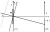 |
Fig. 1 Solar light coming from the (α, β) direction produces a tilted plane wave of equation exp(−2iπ(αx + βy)/λ) on the occulter M (plane 1). The Fresnel diffraction pattern is computed at the telescope aperture T, which is set at the distance z from the occulter (plane 2). The representation is a cut of the xOz plane. |
For a sharp-edged circular occulter and an on-axis point source, the elementary geometrical shadow is a dark disc. It becomes an ellipse for an off-axis point source, but the flattening is very small (10-5 for a point at the solar limb, the cosine of 0.25 degree); we assume that the figure remains a circle. We assume that this property of translation invariance is true regardless of the shape and transmission of the occulter. The resulting UPP is therefore the linear sum of shift invariant figures, which corresponds to a convolution, namely that of the occulter shadow with B⊙(x, y). This convolution relationship holds when the elementary shadow is the result of a Fresnel diffraction, as we demonstrate it in a more formal manner below.
2.2. Expression of the UPP in presence of Fresnel diffraction
We use the classical approach of Fourier optics to describe the Fresnel diffraction in an external occulter coronagraph. We follow the notations of Aime et al. (2013) and refer the reader to the reference book of Goodman (2005) for a detailed course in Fourier optics.
In the { x, y, z } coordinate system, all waves are assumed to propagate towards the z-positive direction. Their complex amplitudes are described in transverse planes { x, y } for fixed z values. A wave, whose wavefront is not in a { x, y } plane, is affected by a phase term function of x and y.
The occulter of amplitude transmission t(x, y) is in the plane of origin z = 0, and the telescope aperture is at the distance z, as illustrated in Fig. 1. A point source of the sun is identified by its angular coordinates (α, β) and brightness intensity |A⊙(α, β)|2. Waves coming from different directions of the Sun are incoherent between them.
An on-axis point source at the center of the solar disk produces a plane wave of constant amplitude A⊙(0,0) in the plane z = 0. In all propagations, an implicit phase term exp(2iπz/λ), which is irrelevant for the present study, is ignored. An off-axis point source produces a tilted plane wave of the form A⊙(α, β)exp(−2iπ(αx + βy)/λ). As illustrated in Fig. 1, the phase term corresponds to the distance between the tilted wavefront and the plane of origin at coordinates (x, y), or αx + βy, that is converted into phase-lag. By doing α = β = 0, note that the off-axis expression includes the on-axis one.
Let us first consider the Fresnel diffraction of the on-axis incident wave of complex
amplitude
A⊙(0,0)t(x, y)
just after the occulter. According to the Huygens-Fresnel theory, its complex amplitude
Ψz,0,0(x, y) at the
distance z can be written as 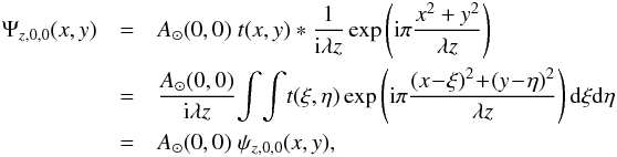 (2)where
the symbol ∗ stands for the two-dimensional convolution on x and
y.
(2)where
the symbol ∗ stands for the two-dimensional convolution on x and
y.
The quantity
ψz,0,0(x, y)
is a characteristic of the diffraction of the occulter at the distance z.
In the present study, we are concerned by intensities, and we denote the OFP as its
modulus squared: 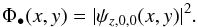 (3)For the off-axis
wave of expression
A⊙(α, β)exp(−2iπ(αx + βy)/λ)t(x, y),
its complex amplitude Ψz, α, β(x, y) at the
distance z can be written as
(3)For the off-axis
wave of expression
A⊙(α, β)exp(−2iπ(αx + βy)/λ)t(x, y),
its complex amplitude Ψz, α, β(x, y) at the
distance z can be written as 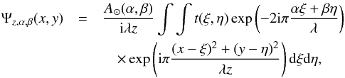 (4)which
can be rewritten as
(4)which
can be rewritten as 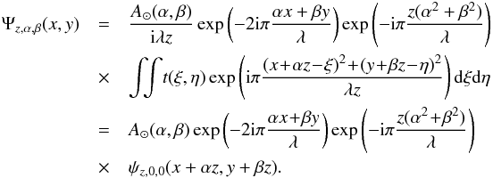 (5)An
off-axis point source produces a complex amplitude shift of the quantity
(αz, βz) towards negative (x, y) directions compared to
the on-axis point-source, as expected from Fig. 1.
The constant phase term accounts for the offset of position, and the original tilt of the
wave is conserved. The intensity due to a point source at position (α, β)
in the z-plane simply becomes
(5)An
off-axis point source produces a complex amplitude shift of the quantity
(αz, βz) towards negative (x, y) directions compared to
the on-axis point-source, as expected from Fig. 1.
The constant phase term accounts for the offset of position, and the original tilt of the
wave is conserved. The intensity due to a point source at position (α, β)
in the z-plane simply becomes  (6)As for the geometrical
approach, the resulting UPP
Uz(x, y) is obtained by
incoherently summing the intensities for all α and β
point sources:
(6)As for the geometrical
approach, the resulting UPP
Uz(x, y) is obtained by
incoherently summing the intensities for all α and β
point sources: 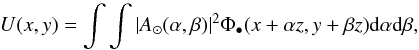 (7)which is an
expression that corresponds to a relation of convolution. This expression can be written
more conveniently if we substitute to the angular intensity
|A⊙(α, β)|2 with its projected
virtual image B⊙(x,y) already defined. We
have considered the inversion of sign in the projected image:
(7)which is an
expression that corresponds to a relation of convolution. This expression can be written
more conveniently if we substitute to the angular intensity
|A⊙(α, β)|2 with its projected
virtual image B⊙(x,y) already defined. We
have considered the inversion of sign in the projected image: 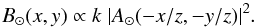 (8)We moreover normalize
the proportionality factor, so that
B⊙(x, y) ∗ 1 = 1. Reporting this expression in
the integral, we demonstrate the convolution relationship of Eq. (1):
(8)We moreover normalize
the proportionality factor, so that
B⊙(x, y) ∗ 1 = 1. Reporting this expression in
the integral, we demonstrate the convolution relationship of Eq. (1): 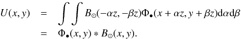 (9)This
relation is valid for any shape and transmission of the occulter, provided that it is set
in a single plane (e.g. in the z = 0 plane). Now, we simplify the problem
to circular symmetric occulters, as defined by a radial function.
(9)This
relation is valid for any shape and transmission of the occulter, provided that it is set
in a single plane (e.g. in the z = 0 plane). Now, we simplify the problem
to circular symmetric occulters, as defined by a radial function.
3. OFPs and UPPs for a circular symmetric occulter of variable transmission
In the previous section, we have established the general relation for obtaining the UPP of
an occulter of arbitrary transmission t(x, y). We now
simplify the problem assuming that the occulter has a circular symmetric transmission
t(r) with  .
.
For an occulting mask, it is convenient to write its transmission as
t(r) = 1 − f(r), where
f(r) is a function with a compact support such that
f(r) = 0 for
|r| > R. The Fresnel
diffraction at the distance z for a wave of unit amplitude becomes
 (10)This
equation illustrates the well-known result that the diffraction of an opaque mask equals 1
minus the diffraction of a transparent mask. This result is very often called after
Babinet’s theorem, although this theorem was originally concerned with diffraction at a lens
focus for which observed intensities of complementary screens are identical for a Dirac
Delta function at r = 0. In Fresnel diffraction, we have, instead, a
difference of 1 in amplitude, and observed intensities of complementary screens are no
longer similar.
(10)This
equation illustrates the well-known result that the diffraction of an opaque mask equals 1
minus the diffraction of a transparent mask. This result is very often called after
Babinet’s theorem, although this theorem was originally concerned with diffraction at a lens
focus for which observed intensities of complementary screens are identical for a Dirac
Delta function at r = 0. In Fresnel diffraction, we have, instead, a
difference of 1 in amplitude, and observed intensities of complementary screens are no
longer similar.
Expanding the convolution in Eq. (10) and
making use of the circular symmetry of the problem, the complex amplitude
ψ•(r) of the diffracted wave can be written
as  (11)where
J0(r) is the Bessel function of the first
kind.
(11)where
J0(r) is the Bessel function of the first
kind.
This integral is the radial form for the Huygens-Fresnel integral of Eq. (2) and appears as the Hankel transform of f(r)exp(iπr2/λz). The quadratic phase term can be physically interpreted as a diverging lens. The OFP defined by Eq. (3) becomes the radial function Φ•(r) = |ψ•(r)|2.
The UPP U(r) is obtained by computing the two-dimensional convolution in Eq. (1), and we specify that it is to be done not on r but on x and y. This operation can be done numerically by inverse filtering. Taking advantage of the circular symmetry of the problem, we can multiply the Hankel transforms of Φ•(r) and B⊙(r) together and then take an inverse Hankel transform. The inverse Hankel transform is identical to the Hankel transform. This reduces the computation to one dimension, although the numerical Hankel transform is a delicate operation, as described by Lemoine (1994).
Alternatively, we can simplify the convolution integral to the form,  (12)where
R⊙ denotes the radius of the geometric image of the solar disc
B⊙(r).
(12)where
R⊙ denotes the radius of the geometric image of the solar disc
B⊙(r).
3.1. OFPs and UPPs for a sharp-edged circular occulter
For a sharp-edged circular occulter, we simply write f(ξ) = 1 in Eq. (11), which corresponds to a compete obscuration by the disk of radius R. Obtaining the value of ψ•(r) for r = 0 is very simple. We obtain a pure phase-term for ψ•(0) that leads to Φ•(0) = 1; that is, we observe the same intensity in the axis as if the occulter was not there. Poisson in 1815 objected against Fresnel theory, because this result was “offending common sense”. Arago made the experiment and indeed observed the bright point foreseen by Poisson, a corner stone of Fresnel’s diffraction theory.
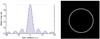 |
Fig. 2 Left: central part of the Arago spot (OFP) for a solar coronagraph at λ = 0.55 μm. The horizontal axis is in microns. Right: focal plane image for a 4 cm diameter telescope set at the center of the OFP of a 1.5 m diameter occulter. |
Obtaining the complete analytic expression for
ψ•(r) for any r value is a
bit more tricky. We derive it in Appendix A, taking
advantage of the approach given in Born & Wolf
(2006). The complex amplitude of the wave at the distance z for
a circular occulter of radius R for the inside
(r < R) and outside
(r > R) of the geometrical
umbra can be written as 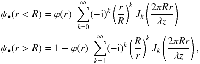 (13)where
ϕ(r) = exp(iπ(r2 + R2)/(λz))
is a quadratic phase term bearing the information that the occulter is at the distance
z from the observing plane. At r = R,
both series converge to the same value given by
(13)where
ϕ(r) = exp(iπ(r2 + R2)/(λz))
is a quadratic phase term bearing the information that the occulter is at the distance
z from the observing plane. At r = R,
both series converge to the same value given by
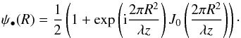 (14)At the center of the
umbra the intensity of the Arago spot for r ≪ R can well
be approximated using only the first term of the series:
(14)At the center of the
umbra the intensity of the Arago spot for r ≪ R can well
be approximated using only the first term of the series: 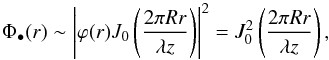 (15)which is an
expression already obtained by Harvey & Forgham
(1984). The distance between the first zeroes of the Arago spot is approximately
1.53λ/α, where
α = 2R/z is the
occulting angle of the coronagraph. For solar observations,
α ~ 1/100 and occulters produce a very tiny spot of
the order of 150λ, or about 80μm, in the visible. A
central cut of the Arago spot and a few surrounding rings is given in Fig. 2.
(15)which is an
expression already obtained by Harvey & Forgham
(1984). The distance between the first zeroes of the Arago spot is approximately
1.53λ/α, where
α = 2R/z is the
occulting angle of the coronagraph. For solar observations,
α ~ 1/100 and occulters produce a very tiny spot of
the order of 150λ, or about 80μm, in the visible. A
central cut of the Arago spot and a few surrounding rings is given in Fig. 2.
A simple physical interpretation of the Arago spot can be drawn by considering the image
given by a telescope of focal length F that receives this wavefront.
Rather than computing the Fourier transform of the Bessel function, it is much easier to
propagate the light in the reverse direction from focus to apertur and to find the
function b(r) whose Fourier transform (here a Hankel
transform) gives the Bessel function in Eq. (15). Thus, we impose the condition, 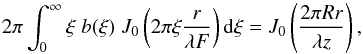 (16)which leads to
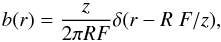 (17)a relation, which
indicates that the edges of the circular occulter are bright and the cause of the Arago
spot. The intensity of the edges is proportional to
(z/R)2; that is it
decreases with the surface of the occulter. We note that the factor
ϕ(r) in Eq. (15) correctly indicates that this image is not exactly at F but
at Fz/(z − F).
(17)a relation, which
indicates that the edges of the circular occulter are bright and the cause of the Arago
spot. The intensity of the edges is proportional to
(z/R)2; that is it
decreases with the surface of the occulter. We note that the factor
ϕ(r) in Eq. (15) correctly indicates that this image is not exactly at F but
at Fz/(z − F).
An example of such an image is given in the right plot of Fig. 2. This result is obtained for an exact numerical calculation, which propagates the wavefront from the occulter down to the focal plane of the instrument of a 4 cm telescope. This is why the edges are thicker than the simple approximation of the Dirac Delta function in Eq. (17).
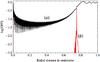 |
Fig. 3 OFP (a) for a circular occulter of 1.5 cm diameter and z = 1.5 m, and corresponding error (b) deduced from Leibniz’s estimate limiting to 100 terms the infinite series in Eq. (13). |
Sums in Eq. (13) are infinite sums that can be computed to a finite number of terms only. The convergence is fast for low r and small R/z values. This is a bit more difficult to achieve for large R/z values, especially in the vicinity of the transition zone (r = R), where the ratio r/R becomes close to 1 and the terms of high k values in Eq. (13) are not rapidly negligible. These series are alternate series for the real and imaginary terms (successive terms are positive and negative). An upper bound of the error for a computation limited to N terms is given by the absolute value of the N + 1 term, according to Leibniz estimate. An example of the estimated error is given in Fig. 3, where we have represented the result obtained for the modulus of the residual complex amplitude in the shadow of a sharp-edged and very small circular occulter that has a 1.5 cm diameter set at 1.5 m, and the sum of the Lommel series is limited to 100 terms. These values are chosen to make visible the result. The associated error obtained by averaging the moduli of the four following terms (101 to 104) is also given in the figure. This representation clearly shows that the error mainly stands in the region close to r = R.
A major computational problem is the very large number of points required to correctly sample the amplitude of the wave in the shadow zone of an occulter in the meter range. Indeed, we have to take a fraction of the Arago spot as a sampling interval. Taking a step of 15 μm corresponds to having 100 000 points within the direct umbra of a 1.5 m occulter. This sampling rate is probably unnecessary for the present study that is limited to intensities in which the convolution with B⊙(r) smoothes the umbras but will be mandatory for future work where we intend to show the resulting image in the focal plane of a telescope.
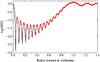 |
Fig. 4 OFP of a disc of 1.5 mm diameter at z = 15 cm. The continuous line represents the Lommel series (Eq. (13)), dots are the result of a direct numerical computation of Eq. (11) using NIntegrate of Mathematica. |
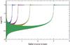 |
Fig. 5 Cut in log scale of 4 OFPs produced by occulters of 0.75 m, 1.5 m, 3 m and 6 m diameters at distances of 69.8 m, 150.4 m, 311.5 m, and 633.8 m, respectively. All curves start at 1 for r = 0. |
An alternative calculation to the Lommel series in Eq. (13) is to numerically compute the fundamental Huygens-Fresnel expression of Eq. (11). This operation involves a discrete Hankel transform, which is a delicate problem, as already indicated. We took advantage of recent improvements of numerical integration in Mathematica (Wolfram 2012), and we found comparable results between the Lommel series and the numerical integration. This is illustrated in Fig. 4 for a simple example with a reasonable number of points and corresponds to the diffraction of a 15 mm disc at a distance of 15 cm. On several other occulter diameters, we have computed the series up to N = 3000; the difference between the result of the series and the direct computation can be as low as 10-15. Obtaining identical results with two entirely different methods makes us confident in the quality of both calculations. The direct computation gives better estimates near r = R, while taking much more computer time. For the calculation using the series, we note that it might be interesting to make the order N to vary with the value of r/R, which would improve both speed of convergence and precision, but this has not been implemented yet in our computation.
In Fig. 5 we give the OFPs Φ•(r) in a logarithm scale, which is produced by occulters of 0.75 m, 1.5 m, 3 m, and 6 m diameters at distances of 69.8 m, 150.4 m, 311.5 m and 633.8 m, respectively. These values correspond to a geometric umbra of 10 cm diameter in all cases. Curves in Fig. 5 may appear as a filling between two envelopes, but this is just a drawing effect due to the huge number of computed values from the sampling interval of 15 μm which leads to more than 260 000 points for the occulter of 6 m diameter. All curves start at 1 for r = 0, as expected, and are very similar for low r values, since the width of the Arago spot does not depend on the occulter diameter and depends only on the obscuration angle, as given by Eq. (15). For larger values of r, the OFP darken when increasing the size of the occulter from about 10-4 of the direct sunlight for the 75 cm occulter to almost 10-5 for a 6 m occulter. Radial cuts of envelopes are U-shaped with the minimum value being roughly at R/2.
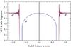 |
Fig. 6 Central slices of a) the OFP Φ•(r) and b) the solar disc B⊙(r), showing the center-to-limb variation normalized to 1 at the center. Parameters used here are: circular occulter of 1.5 m diameter, central dark zone of 0.2 m, distance from the occulter of 139.6 m and wavelength of 0.55 μm. |
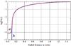 |
Fig. 7 UPPs computed for a Sun of uniform brightness. The (a) geometric UPP is zero inside a disc of 20 cm diameter, while the (b) Fresnel UPP is just below 10-4 of the direct sunlight. Curves are almost identical in the penumbra. Parameters are those of Fig. 6. |
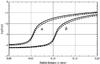 |
Fig. 8 Central part of UPPs produced by a circular occulter of 1.5 m for a geometrical umbra of a) 10 cm diameter and b) 20 cm diameter for a Sun of uniform brightness (full line) or a center-to-limb darkening (dashed line). |
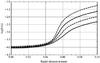 |
Fig. 9 Cuts in the log scale of the UPPs produced by the occulters producing the OFPs as shown in Fig. 5. From upper to lower curves we show occulters of 0.75 m, 1.5 m, 3 m, and 6 m diameters. For all occulters, the diameter of the geometrical umbra is 0.1 m. |
Figure 6 gives a central slice of the OFP in a linear scale for a 1.5 m occulter with a cut of the solar brightness normalized to 1 at the center. Here, the solar photosphere B⊙(r), is represented with a center-to-limb variation given by the function 0.5 + 0.5(1 − (r/R⊙)2)1/2.
Before using this limb darkening, a uniform brightness for B⊙(r) was taken once to directly compare UPPs that are obtained with and without diffraction effects. An example of this is given in Fig. 7, using an occulter of 1.5 m set at a distance of 139.6 m, which provides a geometrical umbra of 20 cm diameter. The function giving the geometrical penumbra, which is the surface of the partially occulted Sun is not given here for the sake of conciseness. It is made of a linear combination of functions used to compute modulation transfer of telescopes (pupil autocorrelation functions). The geometrical and physical penumbras are very similar; the main differences appear for the umbras. Because of diffraction effects, the real umbra that considers diffraction is hardly darker than 10-4 of the direct sunlight, which is unsatisfactory for observation of the solar corona close to the limb.
In Fig. 8, we have illustrated the effect of the center-to-limb variation in the solar photosphere on UPPs. The difference between uniform brightness of the solar disk and a center-to-limb darkening is significant but not very strong. All curves from here are computed by considering the above defined center-to-limb variation. Other functions may be used, if necessary, but the result will not be very decisively modified.
In Fig. 9, we give a central cut of the UPPs obtained with occulter diameters of 0.75 m, 1.5 m, 3 m and 6 m set at distances of 69.8 m, 150.4 m, 311.5 m, and 633.8 m, respectively. These distances are chosen to keep a geometrical umbra of 10 cm in all cases. Corresponding OFPs are those given in Fig. 5. We note that the larger the occulter, the darker the umbra, but the gain in darkness from 0.75 m to 6 m is disappointing (only 30%). The main interest of increasing the diameter of the occulter in this size range is to observe the corona closer to the limb. As a rule of thumb, a simple geometrical approach shows that the angular loss in minutes is 16/(2R/D − 1) for the Sun with angular diameter of 32 arcmin, where D is the diameter of the umbra at the aperture of the telescope. For the 0.75 m, 1.5 m, 3 m, and 6 m diameters, the angular loss of the lower corona is of about 2.46, 1.14, 0.55, and 0.27 min of arc to the limb for the geometrical umbra of 10 cm.
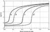 |
Fig. 10 Central part of UPPs produced by a circular occulter of 1.5 m for a geometrical umbra of: a) 10 cm, b) 20 cm, (c) 40 cm, and (d) 60 cm diameter. |
In Fig. 10, we give the level of the residual intensity in the shadow obtained by increasing the value of D from 10 cm to 20 cm, 40 cm, and 60 cm. Corresponding occulter-telescope distances are 150.4 m, 139.6 m, 118.2 m, and 96.7 m, respectively. A darker umbra is obtained at the expense of a loss of observation of the lower corona from 1.14 to 2.46, 5.8, and 10.6 min of arc to the solar limb.
For whatever the configurations, the desired rejections for UPPs are not obtained close enough to the limb, and the needed factor (one hundred or so) is so large that we can conclude that raw circular occulters in the range of a few meters are unlikely to give satisfactory results.
3.2. OFPs and UPPs for an apodized circular occulter
In the present section, we consider apodized occulters with amplitude transmission
t(r) = 1 − f(r),
where the function f(r) is defined by 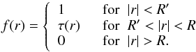 (18)The
function τ(r) is assumed to monotonously decrease from 1
to 0 between R′ and R. Finding the optimal
shape for τ(r) is a problem that was investigated by
Wasylkiwskyj & Shiri (2011) for exoplanet
studies. These authors optimize a polynomial profile for the occulter, and they found an
impressive improvement going from a fourth order polynomial profile to a fortieth one. The
values of R and R′ in which
R′ = R/3 that they
consider cannot fit the solar experiment, where we seek the difference of
R − R′ to be as small as possible. In the
present study, we have empirically considered three kinds of profiles, postponing the
optimization for solar external occulters for future work.
(18)The
function τ(r) is assumed to monotonously decrease from 1
to 0 between R′ and R. Finding the optimal
shape for τ(r) is a problem that was investigated by
Wasylkiwskyj & Shiri (2011) for exoplanet
studies. These authors optimize a polynomial profile for the occulter, and they found an
impressive improvement going from a fourth order polynomial profile to a fortieth one. The
values of R and R′ in which
R′ = R/3 that they
consider cannot fit the solar experiment, where we seek the difference of
R − R′ to be as small as possible. In the
present study, we have empirically considered three kinds of profiles, postponing the
optimization for solar external occulters for future work.
We have represented examples in Fig. 11 of three
transmission functions τ(r) of the form 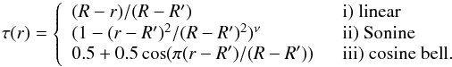 (19)The
drawback of this increase in size of the occulter is that it induces a correlative loss in
the observation of the lower corona. In the example of Fig. 11, the original size of the 1.50 m occulter is increased to 1.53 m, inducing a
loss of less than half an arc minute to the limb. With the notations used, we have
R = 76.5 cm and R′ = 75 cm. In Fig. 12 we give examples of OFPs obtained using the three
apodization functions that are given in Eq. (19). These includes linear, cosine bell and Sonine transmission with
ν = 2.
(19)The
drawback of this increase in size of the occulter is that it induces a correlative loss in
the observation of the lower corona. In the example of Fig. 11, the original size of the 1.50 m occulter is increased to 1.53 m, inducing a
loss of less than half an arc minute to the limb. With the notations used, we have
R = 76.5 cm and R′ = 75 cm. In Fig. 12 we give examples of OFPs obtained using the three
apodization functions that are given in Eq. (19). These includes linear, cosine bell and Sonine transmission with
ν = 2.
The gain factor with respect to the raw occulter is impressive. The Arago spot no longer exists, and the darkness of the shadow is much deeper. Instead of 1 for the raw circular occulter, we have now for r = 0 an intensity of 2.47 × 10⁻⁷ for the linear transmission, 1.81 × 10⁻¹⁰ for the Sonine (with ν = 2), and 1.23 × 10⁻¹⁰ for the cosine bell window. The factor of gain in comparison to the raw circular occulter is of the order of 104 for the linear variation, which is up to 108 for the Sonine and cosine bell transmissions. Shapes of curves are different from before; the minimum intensity of OFPs are closer to the center of the pattern.
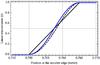 |
Fig. 11 Transmission of the occulter t(r) in the outer 1.5 cm between radii R = 75 cm and R′ = 76.5 cm of the 1.53 m occulter for three functions τ(r): linear, Sonine of parameter ν = 2 (dashed curve), and cosine bell window. |
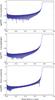 |
Fig. 12 Cuts of OFPs in logarithmic scale for the 1.50 m external occulter enlarged to 1.53 m with an apodization zone. From top to bottom, the transmission at the edge τ(r) is linear, a cosine bell, and a Sonine with ν = 2, as given in Eq. (19) and shown in Fig. 11. |
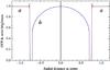 |
Fig. 13 Same representation as in Fig. 6 for the 153 cm Sonine – apodized occulter. Central slices of (a) OFP and (b) solar center-to-limb darkening. |
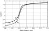 |
Fig. 14 Log-scale representation of cuts of the central part of UPPs produced by external occulters with Sonine apodizations (ν = 2) which exceeds the 150 cm occulter by a) 3 cm and b) 6 cm. |
To compute the UPP obtained with an apodized occulter, we follow the same procedure as in Sect. 3. In Fig. 13, we give radial cuts of an apodized OFP with the image of the solar disc B⊙(r) in its center. The parameters of the experiment are: a Sonine apodization (Eq. (19), ii) with ν = 2), an occulter of 153 cm, and R − R′ = 1.5 cm. The improvement of the OFP using apodization is already visible in this linear scale when comparing it to Fig. 6.
In Fig. 14, we give UPPs obtained for two Sonine – apodized occulters of 153 cm and 156 cm with ν = 2 and R − R′ = 1.5 cm and 3 cm, respectively. As can be seen, there is a tremendous improvement of the darkness depth obtained by these apodized occulters by obstructing just 2 and 4 percent more of the Sun compared to the raw sharp-edged circular occulter.
In Fig. 15 we compare UPPs obtained using raw, linear and Sonine apodized occulters for two sizes of the direct geometric umbra of 10 cm and 20 cm, respectively. Curves obtained with the cosine bell apodizations are very similar to those of the Sonine apodization and are not represented here.
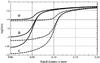 |
Fig. 15 Log-scale representation of cuts of the central part of UPPs produced by external occulters for geometrical umbras of 10 cm (full lines) and 20 cm (dashed lines). a) Raw disc of 150 cm, b) linear apodized occulter of 153 cm, c) Sonine – apodized occulter of 153 cm. See Fig. 11 for apodization profiles. |
Finally, we present a first test of the effect of an occulter with an imperfect transparency in Fig. 16. Our approach considers only defaults of a radial nature into τ(r). Most probably, defaults of realization are more complex, or at least two-dimensional. Nevertheless, such a computation is a first check of the effects of a non perfect transmission, which is probably pessimistic, because the defects are made circular by the calculation technique. The error we introduced in the examples given in Fig. 16 is a discretization with a finite number of levels of the function τ(r). This results in a stepped profile on 10 and 100 levels for the Sonine transmission. This transmission is not represented here.
The result is indeed very sensitive to the smoothness of the occulter, as expected. Instead of the theoretical 10-10 rejection of the perfect Sonine apodization, we obtain only 10-5 for the stepped profile with 10 levels but almost 10-7 for the stepped profile with 100 levels. It is interesting to note that results in both cases remain much better than the 10-4 performance obtained with a raw circular occulter.
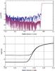 |
Fig. 16 Effect of a stepped profile of τ(r) using a 1.53 m occulter with a Sonine transmission of parameter ν = 2. Top: OFPs for 10 and 100 levels. Bottom: corresponding central part of UPPs produced by these occulters: full line (100 levels), dashed line (10 levels). |
4. Discussion and conclusion
As already indicated, the present study is limited to the computation of the solar umbral pattern at the aperture of the telescope. Obtaining the final intensity in the focal plane would require a more delicate computation that will be considered for future work. Indeed, point spread responses for different points of the Sun will be all different in the telescope focal plane. We no longer have the relation of convolution as has been used, such as in Aime (2007), to derive the expression of the diffraction halo caused by the solar disk, and we will have to work with a Fredholm integral. To be fully realistic, this calculation should also consider the exact nature of the point spread function of the telescope and not just an ideal model.
Several important results have been obtained in our work. We have shown that the solar umbral pattern produced by an occulter of any shape and transmission on the telescope aperture can be written as a convolution relationship between the OFP (optical Fresnel pattern) and the geometric image of the Sun that is given by a perfect pinhole camera for the distance occulter-telescope.
We have obtained an analytic expression for the complex amplitude of the wave diffracted by a circular occulter in the form of Lommel series (Eq. (13)) and briefly discussed the convergence of these alternate series. This complex amplitude can be used as a reference for numerical computations using an external occulter, which includes coronagraphs intended for exoplanet detections. Taking the squared modulus of this complex amplitude gives the OFP Φ•(r). Attention is drawn to the huge number of points required for a correct sampling of the curve of the order of 100 000 points for a 1.5 m occulter.
We have verified that a numerical computation of the Hankel transform (Eq. (11)), which appears in the Huygens-Fresnel integral performed with the function NIntegrate of Mathematica, yields the same result as the Lommel series. It is very comforting to have obtained identical results by two different methods. Attention is drawn to the reader that repeats the calculation with a classical language (such as C or FORTRAN). The numerical Hankel transform is a delicate transform that requires non-uniform sampling based on the zeroes of the Bessel function, as discussed by Lemoine (1994) and other papers of this author.
Using a center-to-limb variation for B⊙(r), we have derived the value of the UPP (solar umbral pattern) U(r) by means of a convolution relationship. Considering the symmetries of the problem, we have reduced the convolution relationship to a simpler integral (Eq. (12)).
It is shown that the UPP obtained using circular occulters hardly goes below 10-4 of the direct sunlight, even if occulters as large of 6 m are considered. It is more efficient to position the telescope closer to the occulter and deeper into its shadows, although the ability to observe the solar corona near the limb then becomes unachievable. Even in these limiting conditions, the rejection rates are much less than what is needed.
Making use of the numerical approach, we have computed the OFP for apodized occulters with a variable transmission over a few centimeters on the edges of a 1.5 m circular occulter. We have compared three transmissions, which includes a linear one and two smoother ones. Results are impressive, since a cosine bell window or a Sonine with ν = 2 makes it possible to lower the level of residual light down to 10-10 of the direct sunlight.
Apodization transmissions investigated here have been chosen on an empirical basis, and we leave the search for optimal functions for future work. Moreover, it is probably very difficult to achieve in practice the optimal transmission. We have given a first test of this problem using stepped profiles for the occulter. The sensitivity to error is high but not as strong as in the case of a pupil apodization, which is used to reduce diffraction wing in the sense of Jacquinot & Roizen-Dossier (1964).
It may be interesting to note that the effect of apodization for a telescope aperture or for an external occulter are opposite. For a telescope with an apodized aperture, as shown in Aime (2005), the expected effect of apodization is to lower the wings of the point spread function with the drawback of an increase in the central part of the diffraction pattern. Therefore the crucial part is the high frequencies of the Fourier transform of the aperture. In contrast, the focus for external occulters is the central zone of diffraction, which concerns low frequencies of the Fresnel transform. This may explain why the external occulter appears less sensitive to transmission faults than the apodized telescope if the difference between Fourier and Fresnel transforms is considered.
Experimentation with apodized occulters is mandatory. If the realization of these variable transmissions eventually proves technically unachievable, the shaped occulters will appear as the necessary substitute. While these shaped occulters are less efficient than occulters with a variable transmission, as discussed by Wasylkiwskyj & Shiri (2011) for exoplanetary studies, they may nevertheless give a sufficient rejection for an external solar coronagraph.
Whether results obtained in the search for exoplanets can be extended to the solar case, the use of petal-shaped occulters with an optimized contour will be better than serrated edge occulters. The OFPs of these shaped occulters are two-dimensional, and the calculation of corresponding OFPs and UPPs require a two-dimensional treatment, unless clever approximations can be made. The optimization of shapes for the solar case will be different than that for exoplanet because constraints are different. This is a study we intend to perform in the near future.
Acknowledgments
Thanks are due to Serge Koutchmy, Yves Rabbia, Alexis Carlotti, and Rémi Flamary for interesting discussions. Particular thanks are due to Yves Rabbia for his careful reading of the manuscript. Thanks are also due to the anonymous referee for very constructive comments.
References
- Aime, C. 2005, A&A, 434, 785 [NASA ADS] [CrossRef] [EDP Sciences] [Google Scholar]
- Aime, C. 2007, A&A, 467, 317 [NASA ADS] [CrossRef] [EDP Sciences] [Google Scholar]
- Aime, C., Carlotti, A., & Rabbia, Y. 2012, eds. S. Boissier, P. de Laverny, N. Nardetto, et al., 491 [Google Scholar]
- Aime, C., Aristidi, E., & Rabbia, Y. 2013, EAS Publ. Ser., 59, 37 [CrossRef] [EDP Sciences] [Google Scholar]
- Arenberg, J. W., Lo, A. S., Glassman, T. M., & Cash, W. 2007, C.R. Physique, 8, 438 [Google Scholar]
- Born, M., & Wolf, E. 2006, Principles of Optics, 7th edn. (Cambridge University Press), 484 [Google Scholar]
- Brueckner, G. E., Howard, R. A., Koomen, M. J., et al. 1995, Sol. Phys., 162, 357 [NASA ADS] [CrossRef] [Google Scholar]
- Cash, W. 2006, Nature, 442, 51 [NASA ADS] [CrossRef] [PubMed] [Google Scholar]
- Evans, J. W. 1948, J. Opt. Soc. Am., 88, 1083 [NASA ADS] [CrossRef] [Google Scholar]
- Goodman J. W. 2005, Introduction to Fourier Optics (Roberts and Company Publishers) [Google Scholar]
- Harvey, J. E., & Forgham, J. L. 1984, Am. J. Phys., 52, 243 [NASA ADS] [CrossRef] [Google Scholar]
- Jacquinot, P., & Roizen-Dossier, B. 1964, Prog. Opt., 3, 31 [Google Scholar]
- Koutchmy, S. 1988, Space Sci. Rev., 47, 95 [CrossRef] [Google Scholar]
- Lamy, P., Damé, L., Vivès, S., & Zhukov, A. 2010, SPIE, 7731, 18 [Google Scholar]
- Lemoine, D. 1994, J. Chem. Phys., 101, 3936 [NASA ADS] [CrossRef] [Google Scholar]
- Lyot, B. 1939, MNRAS, 99, 580 [NASA ADS] [CrossRef] [Google Scholar]
- Marchal, C. 1985, Acta Astron., 12, 195 [CrossRef] [Google Scholar]
- Newkirk, Jr., G., & Bohlin, J. D. 1965, IAU Symp., 23, 287 [Google Scholar]
- Purcell, J. D., & Koomen, M. J. 1962, Coronagraph with Improved Scattered-Light Properties, Report of NRL Progress, US GPO, Washington, D.C. [Google Scholar]
- Vanderbei, R. J., Cady, E., & Kasdin, N. J. 2007, ApJ, 665, 794 [NASA ADS] [CrossRef] [Google Scholar]
- Verroi, E., Frassetto, F., & Naletto, G. 2008, J. Opt. Soc. Am. A, 25, 182 [Google Scholar]
- Vives, S., Lamy, P.,Koutchmy, S., & Arnaud, J. 2009, Adv. Space Res., 43, 1007 [NASA ADS] [CrossRef] [Google Scholar]
- Wasylkiwskyj, W., & Shiri, S. 2011, J. Opt. Soc. Am. A, 28, 1668 [NASA ADS] [CrossRef] [Google Scholar]
- Wolfram 2012, Mathematica (Champaign, IL: Wolfram Research, Inc.) [Google Scholar]
Appendix A: Derivation of the Fresnel diffraction of a circular occulter
An analytic solution to Eq. (11) can be
obtained using an approach similar to the one adopted by Born & Wolf (2006; BW in the
following) for a different problem, which obtains the complex amplitude of the wave in the
vicinity of the focus of a circular lens. To have similar notations to these authors, we
start making the change of variables
u = 2πR2/(λz)
and v = 2πRr/(λz),
so that
u/v = R/r.
The integral in Eq. (11) then takes the
form  (A.1)and is similar to
Eq. (13) page 487 of BW, but with a change of sign in the quadratic phase term. Lommel
(1885) functions Un(u,v) and
Vn(u,v) are used there to
give an analytic form to the integral.
(A.1)and is similar to
Eq. (13) page 487 of BW, but with a change of sign in the quadratic phase term. Lommel
(1885) functions Un(u,v) and
Vn(u,v) are used there to
give an analytic form to the integral.
These functions are defined as  (A.2)and
the value of
u/v = R/r,
which is greater or smaller than 1, determines which function is to be used for ensuring
the convergence of the sum.
(A.2)and
the value of
u/v = R/r,
which is greater or smaller than 1, determines which function is to be used for ensuring
the convergence of the sum.
For r < R, which is inside the
geometric umbra,
v/u < 1. By
making use of Eqs. (20a) and (20b), page 489 of BW, we have, ![\appendix \setcounter{section}{1} \begin{eqnarray} \label{EqA3} &&C(u,v)+{\rm i}S(u,v)=\frac{2}{u} \nonumber\\ &&\qquad\times\left[\sin \left(\frac{v^2}{2 u}\right)+V_0(u,v)\sin\left(\frac{u}{2}\right)-V_1(u,v)\cos\left(\frac{u}{2}\right)\right.\nonumber\\ &&\qquad\left.+{\rm i}\left(\cos\left( \frac{v^2}{2u}\right)-V_0(u,v)\cos\left(\frac{u}{2}\right)-V_1(u,v)\sin\left(\frac{u}{2}\right) \right)\right] \cdot \end{eqnarray}](/articles/aa/full_html/2013/10/aa22304-13/aa22304-13-eq139.png) (A.3)Coming
back from u and v to the original parameters, the
complex amplitude Ψ(r) of Eq. (11) becomes
(A.3)Coming
back from u and v to the original parameters, the
complex amplitude Ψ(r) of Eq. (11) becomes ![\appendix \setcounter{section}{1} \begin{eqnarray} \label{EqA4} \psi_\bullet(r)&=&1+{\rm i} \exp\left({\rm i} \pi \frac{r^2}{\lambda z}\right)\nonumber\\ &&\quad\times\left[ \left(\sin \left(\frac{\pi r^2}{\lambda z}\right)\!+\! \sin\left(\frac{\pi R^2}{ \lambda z}\right)V_0(r,z) \!- \!\cos\left(\frac{\pi R^2}{ \lambda z}\right)V_{1}( r,z)\right)\right.\nonumber\\ &&\left.\quad+{\rm i}\left(\cos \left(\frac{\pi r^2}{\lambda z}\right)\!-\! \cos\left(\frac{\pi R^2}{ \lambda z}\right)V_0(r,z) \!-\! \sin\left(\frac{\pi R^2}{ \lambda z}\right)V_{1}( r,z)\right)\right]. \end{eqnarray}](/articles/aa/full_html/2013/10/aa22304-13/aa22304-13-eq143.png) (A.4)Denoting
ϕ(r) = exp(iπ(r2 + R2)/(λz)),
we obtain the following after some manipulations:
(A.4)Denoting
ϕ(r) = exp(iπ(r2 + R2)/(λz)),
we obtain the following after some manipulations:  (A.5)For
r > R, w use Eqs. (17a) and
(17b), page 488 of BW, and obtain
(A.5)For
r > R, w use Eqs. (17a) and
(17b), page 488 of BW, and obtain  (A.6)Repeating the
calculations in the same way as above, we obtain
(A.6)Repeating the
calculations in the same way as above, we obtain  (A.7)For
r = R, both series converge towards
(A.7)For
r = R, both series converge towards  (A.8)This result can be
obtained as follows. We start by verifying that the two expressions for
r = R converge towards the same value:
(A.8)This result can be
obtained as follows. We start by verifying that the two expressions for
r = R converge towards the same value: ![\appendix \setcounter{section}{1} \begin{eqnarray} \label{Eq9} \exp \left({\rm i} \frac{2 \pi R^2}{ \lambda z}\right)&& \;\sum_{k=0}^\infty (-{\rm i})^kJ_{k}\left( \frac{2 \pi R^2}{ \lambda z}\right)=\nonumber\\[2mm] &&1- \exp\left( {\rm i} \frac{2 \pi R^2}{ \lambda z}\right)\; \sum_{k=1}^\infty (-{\rm i})^k \left( J_{k}\left( \frac{2 \pi R^2}{ \lambda z}\right)\right) \cdot \end{eqnarray}](/articles/aa/full_html/2013/10/aa22304-13/aa22304-13-eq149.png) (A.9)We
use then the fact that
J− k(x) = (−1)kJk(x),
and the Jacobi-Anger relation
(A.9)We
use then the fact that
J− k(x) = (−1)kJk(x),
and the Jacobi-Anger relation  . Performing half the sum of the
two expressions eliminates all terms but k = 0 and leads to the result
given above.
. Performing half the sum of the
two expressions eliminates all terms but k = 0 and leads to the result
given above.
All Figures
|
Fig. 1 Solar light coming from the (α, β) direction produces a tilted plane wave of equation exp(−2iπ(αx + βy)/λ) on the occulter M (plane 1). The Fresnel diffraction pattern is computed at the telescope aperture T, which is set at the distance z from the occulter (plane 2). The representation is a cut of the xOz plane. |
| In the text | |
|
Fig. 2 Left: central part of the Arago spot (OFP) for a solar coronagraph at λ = 0.55 μm. The horizontal axis is in microns. Right: focal plane image for a 4 cm diameter telescope set at the center of the OFP of a 1.5 m diameter occulter. |
| In the text | |
|
Fig. 3 OFP (a) for a circular occulter of 1.5 cm diameter and z = 1.5 m, and corresponding error (b) deduced from Leibniz’s estimate limiting to 100 terms the infinite series in Eq. (13). |
| In the text | |
|
Fig. 4 OFP of a disc of 1.5 mm diameter at z = 15 cm. The continuous line represents the Lommel series (Eq. (13)), dots are the result of a direct numerical computation of Eq. (11) using NIntegrate of Mathematica. |
| In the text | |
|
Fig. 5 Cut in log scale of 4 OFPs produced by occulters of 0.75 m, 1.5 m, 3 m and 6 m diameters at distances of 69.8 m, 150.4 m, 311.5 m, and 633.8 m, respectively. All curves start at 1 for r = 0. |
| In the text | |
|
Fig. 6 Central slices of a) the OFP Φ•(r) and b) the solar disc B⊙(r), showing the center-to-limb variation normalized to 1 at the center. Parameters used here are: circular occulter of 1.5 m diameter, central dark zone of 0.2 m, distance from the occulter of 139.6 m and wavelength of 0.55 μm. |
| In the text | |
|
Fig. 7 UPPs computed for a Sun of uniform brightness. The (a) geometric UPP is zero inside a disc of 20 cm diameter, while the (b) Fresnel UPP is just below 10-4 of the direct sunlight. Curves are almost identical in the penumbra. Parameters are those of Fig. 6. |
| In the text | |
|
Fig. 8 Central part of UPPs produced by a circular occulter of 1.5 m for a geometrical umbra of a) 10 cm diameter and b) 20 cm diameter for a Sun of uniform brightness (full line) or a center-to-limb darkening (dashed line). |
| In the text | |
|
Fig. 9 Cuts in the log scale of the UPPs produced by the occulters producing the OFPs as shown in Fig. 5. From upper to lower curves we show occulters of 0.75 m, 1.5 m, 3 m, and 6 m diameters. For all occulters, the diameter of the geometrical umbra is 0.1 m. |
| In the text | |
|
Fig. 10 Central part of UPPs produced by a circular occulter of 1.5 m for a geometrical umbra of: a) 10 cm, b) 20 cm, (c) 40 cm, and (d) 60 cm diameter. |
| In the text | |
|
Fig. 11 Transmission of the occulter t(r) in the outer 1.5 cm between radii R = 75 cm and R′ = 76.5 cm of the 1.53 m occulter for three functions τ(r): linear, Sonine of parameter ν = 2 (dashed curve), and cosine bell window. |
| In the text | |
|
Fig. 12 Cuts of OFPs in logarithmic scale for the 1.50 m external occulter enlarged to 1.53 m with an apodization zone. From top to bottom, the transmission at the edge τ(r) is linear, a cosine bell, and a Sonine with ν = 2, as given in Eq. (19) and shown in Fig. 11. |
| In the text | |
|
Fig. 13 Same representation as in Fig. 6 for the 153 cm Sonine – apodized occulter. Central slices of (a) OFP and (b) solar center-to-limb darkening. |
| In the text | |
|
Fig. 14 Log-scale representation of cuts of the central part of UPPs produced by external occulters with Sonine apodizations (ν = 2) which exceeds the 150 cm occulter by a) 3 cm and b) 6 cm. |
| In the text | |
|
Fig. 15 Log-scale representation of cuts of the central part of UPPs produced by external occulters for geometrical umbras of 10 cm (full lines) and 20 cm (dashed lines). a) Raw disc of 150 cm, b) linear apodized occulter of 153 cm, c) Sonine – apodized occulter of 153 cm. See Fig. 11 for apodization profiles. |
| In the text | |
|
Fig. 16 Effect of a stepped profile of τ(r) using a 1.53 m occulter with a Sonine transmission of parameter ν = 2. Top: OFPs for 10 and 100 levels. Bottom: corresponding central part of UPPs produced by these occulters: full line (100 levels), dashed line (10 levels). |
| In the text | |
Current usage metrics show cumulative count of Article Views (full-text article views including HTML views, PDF and ePub downloads, according to the available data) and Abstracts Views on Vision4Press platform.
Data correspond to usage on the plateform after 2015. The current usage metrics is available 48-96 hours after online publication and is updated daily on week days.
Initial download of the metrics may take a while.