| Issue |
A&A
Volume 558, October 2013
|
|
|---|---|---|
| Article Number | A108 | |
| Number of page(s) | 9 | |
| Section | Extragalactic astronomy | |
| DOI | https://doi.org/10.1051/0004-6361/201322189 | |
| Published online | 14 October 2013 | |
New calibration and some predictions of the scaling relations between the mass of supermassive black holes and the properties of the host galaxies⋆
Department of Engineering, University of Sannio, Piazza Roma 21, 82100 Benevento, Italy
e-mail: feoli@unisannio.it
Received: 1 July 2013
Accepted: 27 July 2013
We present a new determination of the slope and normalization of three popular scaling laws between the mass of supermassive black holes and stellar velocity dispersion, bulge mass and kinetic energy of the host galaxies. To this aim we have collected 72 objects taken from three different samples and we have used three fitting methods applying the statistical analysis also to the subset of early type galaxies and spirals separately. We find that the relation involving kinetic energy has a slightly better χ2 and linear correlation coefficient than the other two laws. Furthermore, its Hertzsprung-Russell-like behavior is confirmed by the location of young and old galaxies in two different parts of the diagram. A test of its predictive power with the two giant galaxies NGC 3842 and NGC 4889 shows that the mass of the black hole inferred using the kinetic energy law is the closest to the experimental value. The subset of early type galaxies satisfies the theoretical models regarding the black hole mass vs stellar velocity dispersion relation, better than the full sample.
Key words: black hole physics / galaxies: general / galaxies: kinematics and dynamics / galaxies: active / galaxies: statistics / galaxies: evolution
Tables 1 and 7 are available in electronic form at http://www.aanda.org
© ESO, 2013
1. Introduction
About twenty years ago the first supermassive black holes (SMBHs; M• > 106 M⊙) were discovered at the center of some galaxies near the Milky Way (Kormendy & Richstone 1995; Richstone et al. 1998). Then a lot of these objects were found and their number has rapidly increased in the last decade, making possible to collect a statistically meaningful sample of measures of the SMBH masses. Starting from the knowledge of the structural and kinematical parameters of the host galaxies it has been possible to study the correlations between SMBHs and the properties of the corresponding galaxies. Thanks to some catalogs of these experimental measures (Magorrian et al. 1998; Tremaine et al. 2002; Marconi & Hunt 2003; Gebhardt et al. 2003; Häring & Rix 2004; Aller & Richstone 2007; Graham 2008a,b; Hu 2008; Kisaka et al. 2008; Feoli & Mancini 2009; Gültekin et al. 2009a), the astrophysical community identified a large number of scaling laws, in which the mass of SMBHs is related with several properties of the host spheroidal component1, such as for instance bulge luminosity, mass, effective radius, central potential, dynamical mass, concentration, Sersic index, binding energy, etc. (Richstone et al. 1995; Magorrian et al. 1998; Ferrarese & Merritt 2000; Gebhardt et al. 2000; Laor 2001; Merritt & Ferrarese 2001; Wandel 2002; Tremaine et al. 2002; Marconi & Hunt 2003; Häring & Rix 2004; Graham & Driver 2005; Feoli & Mele 2005; Aller & Richstone 2007; Hopkins et al. 2007b). This trend is going on and recently we have proposed, for example, a scaling law M• − Reσ3 (Feoli & Mancini 2011), which is based on a pure theoretical framework, on the wake of the numerical results of Hopkins et al. (2007a), and other groups of researchers have presented relations between M• and X-ray luminosity, radioluminosity (Gültekin et al. 2009b), momentum parameter (Soker & Meiron 2011), number of globular clusters (Burkert & Tremaine 2010; Snyder et al. 2011). Even a correlation with the dark matter halo has been studied but it is still a matter of controversy (Ferrarese 2002; Baes et al. 2003; Kormendy & Bender 2011; Graham 2011; Volonteri et al. 2011; Bellovary et al. 2011).
All these scaling laws have led to the belief that SMBH growth and bulge formation regulate each other (Ho 2004). Furthermore, just as the Faber–Jackson relation, the “traditional” relation between the SMBH mass and bulge velocity dispersion σ or bulge mass Mb should be projections of the same fundamental plane relation. Current observations require a correlation of the form  over a simple correlation with either σ or Mb at ≥3σ confidence (Hopkins et al. 2007a; Hopkins 2008; Marulli et al. 2008).
The debate about the meaning of these scaling laws is still alive, both on the theoretical point of view, i.e. models and simulations (Silk & Rees 1998; Burkert & Silk 2001; King 2003; Wyithe & Loeb 2003; Granato et al. 2004; Sazonov et al. 2005; Begelman & Nath 2005; Croton et al. 2006; Pipino et al. 2009; Di Matteo et al. 2005; Ciotti et al. 2009; Booth & Schaye 2009; Shin et al. 2010; Degraf et al. 2011) and on the experimental one, i.e. measures and statistical elaborations (Beifiori et al. 2009a,b; Park et al. 2012; Graham 2012; Lahav et al. 2011; Li et al. 2012; Sani et al. 2011; Booth & Schaye 2011; Sadoun & Colin 2012; Hopkins et al. 2012; Hopkins 2012).
Recently McConnell et al. (2011) have published the masses of two huge black holes in the center of the galaxies NGC 3842 and NGC 4889. They argued that those masses “are significantly more massive than predicted by linearly extrapolating the widely-used correlations between black hole mass and the stellar velocity dispersion or bulge luminosity of the host galaxy” This is another good reason to investigate the predictive power of other scaling relations different from the widely-used ones studied by McConnell et al. (2011).
In fact, we focus our attention on a very competitive correlation (as well as the popular M• − Mb and M• − σ) between M• and the kinetic energy of random motions of the corresponding bulges, i.e. Mbσ2 that was proposed in 2005 (Feoli & Mele 2005). This relation has also a plausible physical interpretation that resembles the H–R diagram (Feoli & Mancini 2009): the mass of the central SMBH, just like entropy, can only increase with time or at most remain the same but never decrease; M• is therefore related to the age of the galaxy. On the other hand, the kinetic energy of the stellar bulges directly determines the temperature of the galactic system. The validity of the M• − Mbσ2 relation, as a predictor of the SMBH mass in the center of galaxies, has been already tested, with clear positive results, using several independent galaxy samples (Feoli & Mele 2005, 2007; Feoli & Mancini 2009, 2011; Mancini & Feoli 2012) and in the framework of the ΛCDM cosmology (Feoli et al. 2011), using two galaxy formation models based on the Millennium Simulation, one (the Durham model) by Bower et al. (2006) and the other (the MPA model) by De Lucia & Blaizot (2007) .
The present work has two objectives: to give an update recalibration of the above cited scaling relations that involve bulge properties (kinetic energy M• − Mbσ2, bulge mass M• − Mb, and stellar velocity dispersion M• − σ laws) as an extension and a further elaboration of our previous works on this subject, and to show the consequences of the use of the scaling law M• − Mbσ2 in the place of M• − σ in inferring the SMBH masses of the two giant galaxies studied by McConnell et al. (2011).
The paper is structured as follows. In the next section we give some useful definitions, in Sect. 3 we describe the galaxy sample examined and the fitting procedures performed to find the best-fitting lines for each of the relationships considered. In Sect. 4 we report the fitting parameters and show the plot of the black hole mass vs. kinetic energy relation. After that we draw our conclusions in Sect. 5.
2. Definitions
Before examining the details of the sample of experimental data and the results of the fitting procedure, it seems useful to specify some definitions. In particular, the velocity dispersion can be defined in different ways. One can simply use the central value of velocity dispersion σc or take an average inside a certain radius (for example the effective radius Re) weighted with the density distribution of matter ρ(r). So 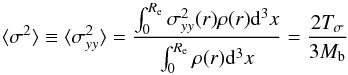 (1)is the luminosity weighted mean of the line of sight component, of the velocity dispersion tensor, assuming that the mass-to-light ratio is constant inside Re and that the tensor is isotropic (Busarello et al. 1992). Tσ is called “kinetic energy of random motions”. The most part of our previous papers on this subject is just on the relationship between the mass of the central black hole and a term
  or Mb ⟨ σ2 ⟩ /c2 proportional to the kinetic energy of random motions.
On the other side, one can consider also V that is the luminosity weighted mean rotation velocity inside Re, defined as 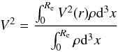 (2)and related to the rotational kinetic energy by TV = MbV2/2 The sum of the two above terms Tσ and TV is the total kinetic energy that can be inserted into the Virial Theorem. The simple scalar version of this theorem is
  (3)where U is the gravitational potential energy and the term Eg = −U is called by definition “gravitational binding energy” (Aller & Richstone 2007). Now, in this paper, we will use the samples of Gültekin et al. (2009a) where an effective dispersion velocity is defined in this way
 ![\begin{equation} \sigma _{\rm e}^{2}=\frac{\int_{0}^{R_{\rm e}}[\sigma^{2}(r) + V^{2}(r)]I(r){\rm d}r}{\int_{0}^{R_{\rm e}}I(r){\rm d}r} \end{equation}](/articles/aa/full_html/2013/10/aa22189-13/aa22189-13-eq33.png) (4)(where σ(r) is the line of sight velocity dispersion, V(r) the rotation velocity and I(r) the galaxy one-dimensional stellar surface brightness profile) The presence, in this particular case, of the rotational component of velocity means that we are studying a relationship between the mass of SMBHs and a term
(4)(where σ(r) is the line of sight velocity dispersion, V(r) the rotation velocity and I(r) the galaxy one-dimensional stellar surface brightness profile) The presence, in this particular case, of the rotational component of velocity means that we are studying a relationship between the mass of SMBHs and a term  proportional to the “total kinetic energy”. Of course, this term can be also interpreted as “gravitational binding energy” if the scalar Virial theorem holds, but this hypothesis is not always verified because often the system under consideration is not really isolated and a term of external pressure must be added in the Eq. (3). As a consequence of this, the bulge masses computed using Virial theorem are often different from the masses estimated using other methods such as the Jeans equation (see Feoli & Mele 2005, for a discussion). This problem will be considered as a source of a possible bias in our results, because the bulge masses of our sample are just determined with different methods. All considered, we prefer to define our law as a relationship between the mass of SMBH and the kinetic energy of the host galaxy and not with its binding energy, well knowing that this is not a real problem but only a theoretical discussion. In practice the effect to change σc with σe or Virial masses with Jeans masses on the resulting scaling relations is very small.
Regression results for log M• = b + mlog x with the full sample composed by 72 galaxies.
3. Data analysis
In order to perform a new calibration and an update of previous results, we have collected 72 galaxies starting from the sample studied by Gültekin et al. (2009a) and adding all the objects (they are 12) from the sample in Hu (2009) not already contained in Gültekin et al. (2009a) and other five spirals from Greene et al. (2010). In order to complete the data for the sample of Gültekin et al. (2009a), we have used the values of bulge masses listed in Table 3 of Feoli et al. (2011), where the corresponding references can be found too. These masses were in part also used in Feoli & Mancini (2009) and have the problem that they are not all determined with the same method (but also black hole masses are often measured with different methods and then put together in the same statistical sample). As already written in previous papers (see, for example the discussion in Feoli & Mancini 2009 Appendix B), we would prefer to have masses computed with Jeans equation as explained, for example, in Häring & Rix (2004), and 25 values of our sample were taken just from that paper, but, in order to construct a more enlarged sample, we have completed the list with other 25 galaxies with Virial dynamical masses and 22 obtained with several photometric approaches from the mass to light ratios. This could generate a bias in the final best fit lines, but the consistency of the results obtained in our previous papers with different samples and fitting methods induces us to believe that this effect must be very small. For example, in Mancini & Feoli (2012), we examined a reduced, but homogeneous sample in which we consider separately stellar masses and dynamical masses and in that case we obtain a very small difference in the slope of our relation from 0.65 to 0.63 respectively, using LYNMIX_ERR and from 0.77 to 0.69 using FITEXY. At the end we will perform a similar check also in this paper, comparing the fit obtained with our sample with the one derived from the use of a new set of bulge masses recently published by Cappellari et al. (2013).
Regression results for log M• = b + mlog x with a subsample composed by 50 early type galaxies.
Regression results for log M• = b + mlog x with a subsample composed by 22 spirals.
In this way we have considered a consistent sample of N = 72 galaxies, which is therefore formed by 33 ellipticals; 13 lenticulars; 4 barred lenticulars; 14 spirals; and 8 barred spirals. By using this sample (all the parameters are reported in Table 1), we want to obtain the slope and the normalization of three popular relationships that can be used to predict the black hole masses in galaxies where the correspondent experimental measures are not available yet. The recalibration could be also useful to develop a consistent theoretical model. As in Gültekin et al. (2009a) and in McConnell & Ma (2013) we have also divided our sample in two subsamples investigating the behaviour of both spirals and early types galaxies, separately.
In particular, the relations that we want to study can be written in the following form  (5)where m is the slope, b is the normalization, and x is a parameter of the host bulge. Equation (5) can be used to predict the values of M• in other galaxies once we know the value of x. In order to minimize the scatter in the quantity to be predicted, we have to perform an ordinary least-squares regression of M• on x for the considered galaxies, of which we already know both the quantities. We considered error bars in both variables and, in order to simplify the analysis, we make all of them symmetric about the preferred value by choosing the maximal value between the upper and lower 1σ error bars for the black hole masses and a constant error for all the bulge masses, so that Δlog 10Mb = 0.18. For the stellar velocity dispersions taken by Greene et al. (2010) we have enlarged the errors in such a way to include the values measured on the major and minor axis and listed in Cols. 3 and 4 of their Table 2. On the other side, we have checked also what happens choosing the opposite way, that is, neglecting errors on both variables. We know that this is an idealized case, because in physics for each measured quantity there is a corresponding error, but we want to perform this kind of test, following the same strategy as our previous paper (Feoli & Mancini 2009), to understand better the weight that the estimation of errors has on the results obtained with our fitting methods. The scaling relations in fact depend critically on the accuracy of the published error estimates in all quantities under consideration (Novak et al. 2006; Lauer et al. 2007).
Hence, to obtain the parameters of our fits (m and b), we have adopted the following two fitting methods and a simple least squared test (LS − TEST).
-
1)
The linear regression routine FITEXY (Presset al. 1992) for the relationy = b + mx, by minimizing the χ2
 (6)
(6) -
2)
The Bayesian linear regression routine LINMIX_ERR (Kelly 2007) to determine the slope, the normalization, and the intrinsic scatter of the relationship
 (7)This routine approximates the distribution of the independent variable as a mixture of Gaussians, bypassing the assumption of a uniform prior distribution on the independent variable, which is used in the derivation of χ2-FITEXY minimization routine. Since a direct computation of the posterior distribution is too computationally intensive, random draws from the posterior distribution are obtained using a Markov Chain Monte Carlo method (Kelly 2007).
 -
3)
The simple least-squares method, used as a test (LS − TEST) in the idealized case of negligible errors on the x and y variables. To this aim, using MATHEMATICA, we obtain simultaneously also the “estimated variance” that corresponds to the square of intrinsic scatter ε0 of the relation and the square of the Pearson linear correlation coefficient.
4. Results
Referring to the sample of 72 galaxies, in Table 2 we collected the parameters of the fits obtained thanks to the two above mentioned fitting methods and the LS test for the various relations that we analyzed, together with the corresponding values of the χ2, the intrinsic scatter ε0, and the Pearson linear correlation coefficient r. In Table 3 and in Table 4 we list the corresponding results for the subsamples of early type galaxies and spirals respectively.
Examining Table 2, it is possible to note that all the fitting parameters are consistent with the previous determinations from the literature. It is also evident that we obtain very similar results using the LYNMIX_ERR routine and using the least squares (LS − TEST) without considering errors in both variables. Different is the behavior obtained by FITEXY that gives always higher slopes, as it has already been shown in our previous works (Feoli & Mancini 2009; Mancini & Feoli 2012). It means that the routine FITEXY is more sensible to the estimation of errors with respect to LYNMIX_ERR.
The  law seems to be preferable if compared with the other relations, especially if one considers the values of
  estimated by FITEXY (Col. 5) or the linear correlation coefficient r (Col. 7). However, the aim of this paper is not to discover what the best among all the correlations is, but only to emphasize that a not widely − used relation such as the
  , is at least as tight as the most famous ones and that in many cases, as for example in Mancini & Feoli (2012), it can offer better predictions than the others. To this aim we have used our relation to infer the masses of the SMBHs in the center of the two giant galaxies NGC 3842 and NGC 4889 that, following McConnell et al. (2011), show “experimental values significantly higher than the ones predicted by the standard M• − σe and M• − L laws”. In particular, in Table 5 and 6 we have reported the black hole masses of NGC 3842 and NGC 4889 respectively, as we have inferred using the law. They are compared with the ones predicted by the M• − σe correlation and with the experimental values. It is evident that our relation infers in both cases a value of mass closer to the experimental one than the one predicted by M• − σe. In particular, our prediction (better for NGC 3842 than for NGC 4889) is such that the interval between the minimal and maximal inferred values overlaps the range of experimental values. It does not occur using the M• − σe law. Furthermore, considering that the experimental value of the mass Mb in the paper of McConnell & Ma (2013) refers only to the stellar mass of the bulge, we think that using the total bulge mass we can obtain with our relation an even better prediction.
Predictions of the black hole mass for the galaxy NGC 3842.
Predictions of the black hole mass for the galaxy NGC 4889.
If we restrict our analysis to the subsample of early type galaxies we can observe that the results obtained in Table 3 match a possible theoretical model (Silk & Rees 1998; Burkert & Silk 2001; King 2003) better than the results obtained by using the full sample. In fact the values of the slopes are closer to integer numbers so that one can guess theoretical laws of this kind:  or
or  , and M• ∝ Mb. It is possible that the early type galaxies dictate the right theoretical model and the spirals create only a small tilt with respect to it. The case of our relation is different, because the fit of the full sample indicates a result close to
  , while the subsample of ellipticals suggests a relation
  , hence the theoretical scenario is still open.
We cannot draw definite conclusions from the subsample composed only by spirals (Table 4), because the results of the slopes are really unstable. For example, if we neglect three galaxies (NGC 2748, NGC 4151, NGC 4258), the slope (LS − TEST) of the M• − σe relation changes from 2.52 to 4.07. In contrast, we note that the intercept remains stable enough changing just from 7.64 to 7.73. The instability is certainly due to the fact that we consider only 22 spirals, a too small sample to have a real statistical meaning. In Table 4, looking at LYNMIX_ERR results, we have obtained, for the relation, values of b and m that are similar to the ones in Table 3 for early type galaxies. In contrast, for M• − σe relation, the values of b and m obtained for spirals are very different with respect to early type galaxies. We expected that the value of m might change because it is very unstable, but we believed that the value of b should remain the same as early type galaxies. However, it did not occur and also b changed with samples of different morphological type. If this result is confirmed using an enlarged sample (for example of the same magnitude of the early types), then the theoretical models developed to explain the M• − σe law must take into account the experimental fact that the proportionality term A in the relation M• = AσB cannot be a constant (composed for example by fundamental constants of nature) but must depend on at least one parameter related to the morphological type of galaxies.
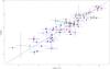 |
Fig. 1
|

Finally we want to be sure that the effect of having collected bulge masses estimated with different methods is very small on the scaling relations. To this aim we perform a test listing in Table 7 all the 33 galaxies in common between the 72 objects in our Table 1 and the set of 260 recently studied by Cappellari et al. (2013). All the masses in Table 7 are estimated with the same method and the details of the measures can be found in the paper (Cappellari et al. 2013). We have computed them using Cols. 6 and 15 of the Cappellari’s Table 1 that allows to find the value of a mass called MJAM defined by the authors as MJAM = (M/L) × L ≃ 5Reσ2/G.
This subsample, formed only by ellipticals and lenticulars, 8 from the original sample of Hu (2009) and 25 from Gültekin et al. (2009a), has been used to find the best fit line of the black hole mass vs bulge mass relation with FITEXY. We obtain with the bulge masses of Cappellari et al. (2013): b = −6.9 ± 1.2 and m = 1.39 ± 0.11, that we have compared to the fit of the corresponding 33 objects with bulge masses taken from our Table 1. It gives b = −7.48 ± 0.78 and m = 1.43 ± 0.07. The result is that slope m and normalization b of the two fits are equivalent inside the errors. We conclude that there is no strong bias in our sample due to the different methods used to estimate the bulge masses.
In Fig. 1, we report the relation in log–log plot (we associated a particular marker to each galaxy according to its morphological type) just to make evident the similarity of the resulting picture with the H–R diagram for stellar evolution. The old elliptical galaxies are generally located in the upper right part of the diagram, while the young spirals and some dwarf ellipticals (NGC 221, NGC 2778, NGC 4486A and NGC 4742) are in the lower left part (the only spiral in the upper right part is the Sombrero galaxy NGC 4594). All the barred galaxies (lenticulars and spirals) are placed in the lower left half of the diagram. Hence the resulting picture confirms the results obtained in Feoli & Mancini (2009) and has a simple interpretation: young galaxies are in the lower left part and old galaxies in the upper right part.
If we go on with comparing the H–R diagram for stars to our relation regarding galaxies, we can see that in the first one the stars move during their life from one zone to another, so we imagine that the same should occur in our diagram as well. However, the last statement should be taken with caution as it needs to be verified. If the galaxies move following the best fit line shown in Fig. 1, as the stars in the H–R diagram do, the resulting scenario is that young dwarf ellipticals, as time goes by and with subsequent mergers, become massive ellipticals, spirals become lenticulars or ellipticals (or spirals with a huge spheroidal component as NGC 4594), while the barred galaxies lose their bars with time: a behavior consistent with theoretical models, that, however, should be tested in details by the experts of simulations. Of course there are some galaxies that are classified in literature (see for example Graham 2008a) also in a different way with respect to the types listed in Table 1 and used for the Fig. 1. For example, NGC 221, NGC 4459, NGC 4564 and NGC 5128 have been defined as E, but also as S0, NGC 2778 as E and also as SB0 and NGC 1194 as S and also as S0. However, even changing the morphological classifications of some galaxies, the above described general trends, shown by the diagram in Fig. 1, do not change.
5. Conclusion
Starting from a sample of 72 galaxies, we have obtained the best fit lines of three popular scaling laws. Among them, we have found that the has a χ2 and a linear correlation coefficient better than the other two. Hence this relation is a good instrument to give predictions of the still unmeasured masses of SMBHs at the center of galaxies whose kinetic energy is known. In order to test the predictive power of the law, we have tried to guess the masses of the Black Holes of the giant galaxies NGC 3842 and NGC 4889. The result is that the value predicted by our relation is closer to the experimental one, with respect to the prediction of the M• − σe law.
Furthermore, our statistical analysis allows to give two suggestions to the authors of theoretical models for the M• − σe law. First, the early types galaxies match well the models, while the spirals seem to play only a marginal role. Secondly, the normalization of the relation does not seem to be a constant but it may depend on the morphological type of galaxies.
Online material
Experimental data for our sample of 72 galaxies.
The subsample of 33 bulge masses, all determined with the same method, by Cappellari et al. (2013).
Acknowledgments
We acknowledges support for this work by research funds of the University of Sannio. Special thanks to Luigi Mancini for the fits with LINMIX_ERR and Rossella Sanseverino for useful suggestions about English.
References
- Aller, M. C., & Richstone, D. O. 2007, ApJ, 665, 120 [NASA ADS] [CrossRef] [Google Scholar]
- Baes, M., Buyle, P., Hau, G. K. T., & Dejonghe 2003, MNRAS, 341, L44 [NASA ADS] [CrossRef] [Google Scholar]
- Begelman, M. C., & Nath, B. B. 2005, MNRAS, 361, 1387 [NASA ADS] [CrossRef] [Google Scholar]
- Beifiori, A., Sarzi, M., Corsini, E. M., et al. 2009a, ApJ, 692, 856 [NASA ADS] [CrossRef] [Google Scholar]
- Beifiori, A., Courteau, S., Corsini, E. M., & Zhu, Y. 2009b, MNRAS, 419, 2497 [Google Scholar]
- Bellovary, J., Volonteri, M., Governato, F., et al. 2011, ApJ, 742, 13 [NASA ADS] [CrossRef] [Google Scholar]
- Booth, C. M., & Schaye, J. 2009, MNRAS, 398, 53 [NASA ADS] [CrossRef] [Google Scholar]
- Booth, C. M., & Schaye, J. 2011, MNRAS, 413, 1158 [NASA ADS] [CrossRef] [Google Scholar]
- Bower, R. G., Benson, A. J., Malbon, R., et al. 2006, MNRAS, 370, 645 [NASA ADS] [CrossRef] [Google Scholar]
- Burkert, A., & Silk, J. 2001, ApJ, 554, L151 [NASA ADS] [CrossRef] [Google Scholar]
- Burkert, A., & Tremaine, S. 2010, ApJ, 720, 516 [NASA ADS] [CrossRef] [Google Scholar]
- Busarello, G., Longo, G., & Feoli, A. 1992, A&A, 262, 52 [NASA ADS] [Google Scholar]
- Cappellari, M., Scott, N., Alatalo, K., et al. 2013, MNRAS, 432, 1709 [NASA ADS] [CrossRef] [Google Scholar]
- Ciotti, L., Ostriker, J. P., & Proga, D. 2009, ApJ, 699, 89 [NASA ADS] [CrossRef] [Google Scholar]
- Croton, D. J., Springel, V., White, S. D. M., et al. 2006, MNRAS, 365, 11 [NASA ADS] [CrossRef] [Google Scholar]
- Degraf, C., Di Matteo, T., & Springel, V. 2011, MNRAS, 413, 1383 [NASA ADS] [CrossRef] [Google Scholar]
- De Lucia, G., & Blaizot, J. 2007, MNRAS, 375, 2 [NASA ADS] [CrossRef] [Google Scholar]
- Di Matteo, T., Springel, V., & Hernquist, L. 2005, Nature, 433, 604 [NASA ADS] [CrossRef] [PubMed] [Google Scholar]
- Feoli, A., & Mancini, L. 2009, ApJ, 703, 1502 [NASA ADS] [CrossRef] [Google Scholar]
- Feoli, A., & Mancini, L. 2011, Int. J. Mod. Phys. D, 20, 2305 [NASA ADS] [CrossRef] [Google Scholar]
- Feoli, A., & Mele, D. 2005, Int. J. Mod. Phys. D, 14, 1861 [NASA ADS] [CrossRef] [Google Scholar]
- Feoli, A., & Mele, D. 2007, Int. J. Mod. Phys. D, 16, 1261 [NASA ADS] [CrossRef] [Google Scholar]
- Feoli, A., Mancini, L., Marulli, F., & van den Bergh, S. 2011, Gen. Rel. Grav., 43, 1007 [NASA ADS] [CrossRef] [Google Scholar]
- Ferrarese, L. 2002, ApJ, 578, 90 [NASA ADS] [CrossRef] [Google Scholar]
- Ferrarese, L., & Merritt, D. 2000, ApJ, 539, L9 [NASA ADS] [CrossRef] [Google Scholar]
- Gebhardt, K., Bender, R., Bower, G., et al. 2000, ApJ, 539, 13 [Google Scholar]
- Gebhardt, K., Richstone, D. O., Tremaine, S., et al. 2003, ApJ, 583, 92 [NASA ADS] [CrossRef] [Google Scholar]
- Graham, A. W. 2008a, PASA, 25, 167 [NASA ADS] [CrossRef] [Google Scholar]
- Graham, A. W. 2008b, ApJ, 680, 143 [NASA ADS] [CrossRef] [Google Scholar]
- Graham, A. W. 2011 [arXiv:1103.0525] [Google Scholar]
- Graham, A. W. 2012, ApJ, 746, 113 [NASA ADS] [CrossRef] [Google Scholar]
- Graham, A. W., & Driver, S. P. 2005, PASA, 22, 118 [NASA ADS] [CrossRef] [Google Scholar]
- Granato, G. L., De Zotti, G., Silva, L., et al. 2004, ApJ, 600, 580 [Google Scholar]
- Greene, J. E., Peng, C. Y., Kim, M., et al. 2010, ApJ, 721, 26 [NASA ADS] [CrossRef] [Google Scholar]
- Gültekin, K., Cackett, E. M., Miller, J. M., et al. 2009a, ApJ, 698, 198 [NASA ADS] [CrossRef] [Google Scholar]
- Gültekin, K., Cackett, E. M., Miller, J. M., et al. 2009b, ApJ, 706, 404 [NASA ADS] [CrossRef] [Google Scholar]
- Häring, N., & Rix, H. 2004, ApJ, 604, L89 [NASA ADS] [CrossRef] [Google Scholar]
- Ho, L. C. 2004, Coevolution of Black Holes and Galaxies, Carnegie Observatories Astrophys. Ser. 1 (Cambridge: Cambridge Univ. Press) [Google Scholar]
- Hopkins, P. F. 2008, in Formation and Evolution of Galaxy Bulges, eds. M. Bureau, E. Athanassoula, & B. Barbuy (Cambridge: Cambridge Univ. Press), IAU Symp., 245, 219 [Google Scholar]
- Hopkins, P. F. 2012, MNRAS, 420, L8 [NASA ADS] [CrossRef] [Google Scholar]
- Hopkins, P. F., Hernquist, L., Cox, T. J., et al. 2007a, ApJ, 669, 45 [NASA ADS] [CrossRef] [Google Scholar]
- Hopkins, P. F., Hernquist, L., Cox, T. J., et al. 2007b, ApJ, 669, 67 [NASA ADS] [CrossRef] [Google Scholar]
- Hopkins, P. F., Hernquist, L., Hayward, C. C., et al. 2012, MNRAS, 425, 1121 [NASA ADS] [CrossRef] [Google Scholar]
- Hu, J. 2008, MNRAS, 386, 2242 [NASA ADS] [CrossRef] [Google Scholar]
- Hu, J. 2009 [arXiv:0908.2028] [Google Scholar]
- Kelly, B. C. 2007, ApJ, 665, 1489 [NASA ADS] [CrossRef] [Google Scholar]
- King, A. R. 2003, ApJ, 596, L27 [NASA ADS] [CrossRef] [Google Scholar]
- Kisaka, S., Kojima, Y., & Otani, Y. 2008, MNRAS, 390, 814 [NASA ADS] [CrossRef] [Google Scholar]
- Kormendy, J., & Bender, R. 2011, Nature, 469, 377 [NASA ADS] [CrossRef] [PubMed] [Google Scholar]
- Kormendy, J., & Richstone, D. 1995, ARA&A, 33, 581 [NASA ADS] [CrossRef] [Google Scholar]
- Lahav, C. G., Meiron, Y., & Soker, N. 2011 [arXiv:1112.0782] [Google Scholar]
- Laor, A. 2001, ApJ, 553, 677 [NASA ADS] [CrossRef] [Google Scholar]
- Lauer, T. R., Faber, S. M., Richstone, D., et al. 2007, ApJ, 662, 808 [NASA ADS] [CrossRef] [Google Scholar]
- Li, N., Mao, S., Gao, L., et al. 2012, MNRAS, 419, 2424 [NASA ADS] [CrossRef] [Google Scholar]
- Mancini, L., & Feoli, A. 2012, A&A, 537, A48 [NASA ADS] [CrossRef] [EDP Sciences] [Google Scholar]
- Marulli, F., Bonoli, S., Branchini, E., et al. 2008, MNRAS, 385, 1846 [NASA ADS] [CrossRef] [Google Scholar]
- Magorrian, J., Tremaine, S., Richstone, D., et al. 1998, AJ, 115, 2285 [NASA ADS] [CrossRef] [Google Scholar]
- Marconi, A., & Hunt, L. K. 2003, ApJ, 589, L21 [NASA ADS] [CrossRef] [Google Scholar]
- McConnell, N. J., & Ma, C. 2013, ApJ, 764, 184 [NASA ADS] [CrossRef] [Google Scholar]
- McConnell, N. J., Ma, C.-P., Gebhardt, K., et al. 2011, Nature, 480, 215 [NASA ADS] [CrossRef] [Google Scholar]
- Merritt, D., & Ferrarese, L. 2001, ApJ, 547, 140 [NASA ADS] [CrossRef] [Google Scholar]
- Novak, G. S., Faber, S. M., & Dekel, A. 2006, ApJ, 637, 96 [NASA ADS] [CrossRef] [Google Scholar]
- Park, D., Kelly, B. C., Woo, J.-H., et al. 2012, ApJS, 203, 6 [NASA ADS] [CrossRef] [Google Scholar]
- Pipino, A., Silk, J., & Matteucci, F. 2009, MNRAS, 392, 475 [NASA ADS] [CrossRef] [Google Scholar]
- Press, W. H., Teukolsky, S. A., Vetterling, W. T., & Flannery, B. P. 1992, Numerical Recipes, 2nd edn. (Cambridge: Cambridge University Press) [Google Scholar]
- Richstone, D., Ajhar, E. A., Bender, R., et al. 1998, Nature, 395, A14 [NASA ADS] [Google Scholar]
- Sadoun, R., & Colin, J. 2012, MNRAS, 426, L51 [NASA ADS] [Google Scholar]
- Sani, E., Marconi, A., Hunt, L. K., et al. 2011, MNRAS, 413, 1479 [NASA ADS] [CrossRef] [Google Scholar]
- Sazonov, S.Yu, Ostriker, J. P., Ciotti, L., et al. 2005, MNRAS, 358, 168 [NASA ADS] [CrossRef] [Google Scholar]
- Schneider, P. 2006, Extragalactic astronomy and cosmology (Heidelberg: Springer-Verlag Berlin) [Google Scholar]
- Shin, M.-S., Ostriker, J. P., & Ciotti, L. 2010, ApJ, 711, 268 [NASA ADS] [CrossRef] [Google Scholar]
- Silk, J., & Rees, M. J. 1998, A&A, 331, L1 [NASA ADS] [Google Scholar]
- Snyder, G. F., Hopkins, P. F., & Hernquist, L. 2011, ApJ, 728, L24 [NASA ADS] [CrossRef] [Google Scholar]
- Soker, N., & Meiron, Y. 2011, MNRAS, 411, 1803 [NASA ADS] [CrossRef] [Google Scholar]
- Tremaine, S., Gebhardt, K., Bender, R., et al. 2002, ApJ, 574, 740 [NASA ADS] [CrossRef] [Google Scholar]
- Volonteri, M., Natarajan, P., & Gultekin, K. 2011, ApJ, 737, 50 [NASA ADS] [CrossRef] [Google Scholar]
- Wandel, A. 2002, ApJ, 565, 762 [NASA ADS] [CrossRef] [Google Scholar]
- Wyithe, J. S. B., & Loeb, A. 2003, ApJ, 595, 614 [NASA ADS] [CrossRef] [Google Scholar]
All Tables
Regression results for log M• = b + mlog x with the full sample composed by 72 galaxies.
Regression results for log M• = b + mlog x with a subsample composed by 50 early type galaxies.
Regression results for log M• = b + mlog x with a subsample composed by 22 spirals.
The subsample of 33 bulge masses, all determined with the same method, by Cappellari et al. (2013).
All Figures
|
Fig. 1
|
| In the text | |
Current usage metrics show cumulative count of Article Views (full-text article views including HTML views, PDF and ePub downloads, according to the available data) and Abstracts Views on Vision4Press platform.
Data correspond to usage on the plateform after 2015. The current usage metrics is available 48-96 hours after online publication and is updated daily on week days.
Initial download of the metrics may take a while.