| Issue |
A&A
Volume 558, October 2013
|
|
|---|---|---|
| Article Number | A64 | |
| Number of page(s) | 7 | |
| Section | Interstellar and circumstellar matter | |
| DOI | https://doi.org/10.1051/0004-6361/201321896 | |
| Published online | 03 October 2013 | |
Constraints on the radial distribution of the dust properties in the CQ Tauri protoplanetary disk
1 Department of Physics and Astronomy, University of Bologna, viale Berti Pichat 6/2, 40127 Bologna, Italy
e-mail: This email address is being protected from spambots. You need JavaScript enabled to view it.
2 Dipartimento di Fisica e Astrofisica, Universitá degli Studi di Firenze, Largo E. Fermi 2, 50125 Firenze, Italy
3 INAF – Osservatorio astrofisico di Arcetri, Largo E. Fermi 5, 50125 Firenze, Italy
4 ESO, Karl Schwarzschild str. 2, 85748 Garching bei Muenchen, Germany
5 Excellence Cluster Universe, Boltzmannstr. 2, 85748 Garching, Germany
6 Dublin Institute for Advanced Studies, School of Cosmic Physics, 31 Fitzwilliam Place, Dublin 2, Ireland
7 Division of Physics, Mathematics and Astronomy, California Institute of Technology, MC 249-17, Pasadena, CA 91125, USA
Received: 15 May 2013
Accepted: 26 July 2013
Abstract
Context. Grain growth in protoplanetary disks is the first step towards the formation of the rocky cores of planets. Models predict that grains grow, migrate, and fragment in the disk and predict varying dust properties as a function of radius, age, and physical properties. High-angular resolution observations at more than one (sub-)mm wavelength are the essential tool for constraining grain growth and migration on the disk midplane.
Aims. We developed a procedure to analyze self-consistently multiwavelength (sub-)mm continuum interferometric observations of protoplanetary disks to constrain the radial distribution of dust properties.
Methods. We apply this technique to existing multifrequency continuum mm observations of the disk around CQ Tau, a A8 pre-main sequence star with a well-studied disk.
Results. We demonstrate that our models can be used to simultaneously constrain the disk and dust structure. In CQ Tau, the best-fitting model has a radial dependence of the maximum grain size, which decreases from a few cm in the inner disk (<40 AU) to a few mm at 80 AU. Nevertheless, the currently available dataset does not allow us to exclude the possibility of a uniform grain size distribution at a 3σ level.
Key words: protoplanetary disks / stars: pre-main sequence / circumstellar matter / stars: individual: CQ Tauri / dust, extinction / submillimeter: planetary systems
© ESO, 2013
1. Introduction
Planetary systems are relatively common around all types of stars (e.g. Borucki et al. 2011). The origin of planets is intricately tied to the evolution of their primordial protoplanetary disks. The disks provide the reservoirs of raw material and determine the conditions for the formation of planetary systems. A possible evolutionary scenario currently considered for planet formation is the core accretion gas-capture model (see e.g. Lissauer 1993), featuring a build-up of planet cores first and then a gas-infall on sufficiently massive cores later. According to this model, the growth by coagulation from the initial ISM population of sub-micron size dust grains to centimeter sizes is the first step of planet formation.
Spatially resolved observations at sub-(mm) wavelengths of the thermal dust emission from circumstellar disks provide the most direct tool for studying dust properties and thus investigating the very early stages of planet formation. Except for the inner disk region, the dust optical depth at sub-(mm) wavelengths is sufficiently low, so that it is possible at these wavelengths to directly probe the dust grain populations near the disk midplane, where the process of planet formation is supposed to occur.
In the past two decades, several authors have measured the spectral energy distribution (SED) of protoplanetary disks at (sub)-mm wavelengths and found that it is possible to describe it as a power-law with index α (Fν ∝ να), with α being significantly lower in this case than in the diffuse interstellar medium case, where α ~ 3.5−4 (e.g. Beckwith & Sargent 1991; Wilner et al. 2000, 2005; Testi et al. 2001, 2003; Natta et al. 2004; Andrews & Williams 2005; Rodmann et al. 2006; Lommen et al. 2007, 2009; Ricci et al. 2010a,b, 2011). Assuming optically thin emission and a Rayleigh-Jeans approximation, α is directly linked to the spectral index β of the dust opacity coefficient, where kν ∝ νβ and β = α − 2. In this way, measured low values of α (≲3) translate into a value of β ≲ 1 which can be explained if grains have grown to sizes of at least a few millimeters (see e.g. Draine 2006; Natta et al. 2007).
More recently, spatially resolved, multiwavelength interferometric observations have been carried out for a few disks as a means to study the radial dependence of grain growth (Isella et al. 2010; Banzatti et al. 2011; Guilloteau et al. 2011; Perez et al. 2012). The results indicate a radial dependence of the spectral index β, which appears to increase from low values (in some cases, as low as 0) in the inner disk to about 1.7–2 in the outer disk regions. This is interpreted as a decrease in the maximum grain size as a function of the distance from the central star, from centimeter-size grains in the inner disk to mm-size and smaller grains in the outer disk (typically, ~100 AU). Most of these results are based on the method presented in Isella et al. (2010). The method requires spatially resolved observations at two (or more) (sub)-mm wavelengths, which are independently compared to theoretical disk models to constrain the disk surface density and temperature by assuming a constant dust opacity, or a constant β through the disk. The best-fit models at the different wavelengths are then compared to derive the true radial profile of β and of the grain size distribution and the disk surface density and dust temperature (see, e.g., Peréz et al. 2012).
We propose to constrain the disk structure and the radial variation in the grain size distribution through a more direct approach. We develop a self-consistent disk model that includes a grain size distribution that varies with the distance from the central star. The model is used to investigate the radial dependence of the mm-wave spectral indexes α and β from the variations in the maximum grain size and to calculate the radial profile of the disk emission to compare with the observations.
We apply the model to analyze a set of interferometric observations of the pre-main sequence star CQ Tau. The star CQ Tau is one of the closest (100 pc, Hipparcos, Perryman et al. 1997), young intermediate mass stars surrounded by a circumstellar disk. It is situated in the Taurus-Auriga star forming region and is a well-studied variable star of the UX Ori class with spectral type A8 and an estimated age ~5−10 Myr (e.g. Chapillon et al. 2008). The dust continuum emission from the CQ Tau disk has been studied in detail by several authors in the past. The presence of grain growth to ~cm sizes was inferred from the analysis of the disk SED at mm-wavelengths (Natta et al. 2000; Chiang et al. 2001; Testi et al. 2001, 2003; Chapillon et al. 2008). A multifrequency study of CQ Tau was done by Banzatti et al. (2011), who analyzed high-resolution observations from 0.87 mm to 7 mm obtained at the SMA, IRAM-PdB, and NRAO-VLA interferometers. Assuming a constant dust opacity throughout the disk, they found evidence of evolved dust by constraining the disk-averaged dust opacity spectral index β to be 0.6 ± 0.1. Different surface density profiles are found at different wavelengths, indicating a change of dust properties with radius.They concluded suggesting a radial variation in the slope β of the dust opacity, which is consistent with a degree of grain growth varying across the disk.
In this paper, we simultaneously analyze the three datasets at 1.3, 2.7 and 7 mm used in Banzatti et al. (2011), relax the assumption of radially constant dust opacity and fit the data with a disk model, where the grain size distribution is allowed to vary with the distance to the central star.
The paper is organized as follows: Sects. 2 and 3 contains the description of the adopted disk structure and dust opacity models and some examples of the results. The procedure used to fit the data is described in Sect. 4. In Sects. 5 and 6, we present the results and discuss the possible origin of the fitted maximum grain size radial distribution. The main conclusion of this study are summarized in Sect. 7.
2. Disk model
The gas surface density profile Σg(R) is described by the similarity solution for the disk surface density of a viscous Keplerian disk (Lynden-Bell & Pringle 1974). We adopt the mathematical formulation described in Isella et al. (2009): ![Mathematical equation: \begin{equation} \Sigma_{\rm g}(R,t) = \Sigma_{\rm tr} \left( \frac{R_{\rm tr}}{R} \right)^{\gamma} \exp \left\{ -\frac{1}{2(2-\gamma)} \left[ \left( \frac{R}{R_{\rm tr}} \right)^{(2-\gamma)} - 1 \right] \right\}, \label{eq:selfsimilar_solution} \end{equation}](/articles/aa/full_html/2013/10/aa21896-13/aa21896-13-eq20.png) (1)where Rtr is the transition radius1, Σtr is the surface density at Rtr, and γ is the power law index of the viscosity νt(R) ∝ Rγ. We assume a constant dust-to-gas mass ratio ζ = 0.01 throughout the disk, so that dust surface density Σd is 100 less massive than the gas surface density Σg at each radius R.
(1)where Rtr is the transition radius1, Σtr is the surface density at Rtr, and γ is the power law index of the viscosity νt(R) ∝ Rγ. We assume a constant dust-to-gas mass ratio ζ = 0.01 throughout the disk, so that dust surface density Σd is 100 less massive than the gas surface density Σg at each radius R.
The physical structure and emission of the disk is calculated by adopting the two-layer approximation for the solution of the radiation transfer equation (Chiang & Goldreich 1997), following the procedure presented in Dullemond et al. (2001). The disk is described through a warm surface layer directly heated by the stellar radiation and a cooler midplane interior heated by the radiation reprocessed by the surface layer. Both temperatures are calculated as a function of the orbital radius by assuming that the disk is in hydrostatic equilibrium between the gas pressure and the stellar gravity. This leads to a flared geometry with the opening angle that increases with the distance from the central star. The central star is treated as a blackbody. For CQ Tau, we assume the same stellar properties found in Testi et al. (2003): Teff = 6900 K, L⋆ = 6.6 L⊙M⋆ = 1.5 M⊙, and d = 100 pc.
In the disk interior, we adopt a dust model as found in Banzatti et al. (2011), which consists of porous composite spherical grains made of 7% astronomical silicates, 21% carbonaceous material, 42% water ice, and 30% vacuum. We use the Bruggeman effective medium theory (Bruggeman 1935) to calculate an effective dielettric function ϵeff for the composite grain and then use this function in the Mie theory to derive the dust absorption efficiency Qabs(a,ν). The complex optical constant of individual components are taken from Weingartner & Draine (2001) for astronomical silicates, from Zubko et al. (1996) for carbonaceous material, and from Warren (1984) for water ice. Throughout the entire disk, we consider a grain size distribution parametrized as a truncated power-law with slope q:  (2)truncated between the minimum and maximum grain sizes amin and amax, respectively. The value of amin is set to 5 nm, but the results of our analysis do not depend on the exact value of this parameter as long as amin ≪ 1 mm. For the power law index, we have used q = 3 as proposed in previous studies and theoretical expectations (Draine 2006).
Unlike previous works, we allow the maximum grain size amax to vary with the orbital radius. We adopt a power law profile:  (3)where amax,0 is the maximum grain size value at a reference position R0, and bmax is the power-law exponent. Given the dust absorption efficiency Qabs(a,ν) and the grain size distribution n(a,R), the dust opacity at frequency ν and radius R can be then expressed as
  (4)where ρs is the mean density of composite dust grain given in our case, such that ρs = fsilρsil + fcaρca + ficeρice, where the fi terms are the volume fractions of each species given above.
In the disk atmosphere, we assume a constant grain size distribution characterized by grains smaller than 1 μm. This choice, which does not affect the radial profile of the millimeter-wave disk emission, is motivated because larger grains are thought to settle toward the disk midplane (see, e.g., Dullemond & Dominik 2004).
The disk emission is finally expressed as the sum of the emission from the disk interior  and the disk surface layer
  . These are expressed (see Dullemond et al. 2001), respectively, by
 ![Mathematical equation: \begin{eqnarray} I_{\nu}^{i}(R) &=& \frac{ \cos{i}}{d^2} B_\nu(T_i(R)) \left[ 1 - {\rm e}^{- \frac{\Sigma(R) k^i_\nu(R)}{\cos{i}}} \right] \\ I_{\nu}^{\rm s}(R) &=& \frac{1}{d^2} B_\nu(T_{\rm s}(R)) \Delta \Sigma(R) k_\nu^s(R) \left[ 1 + {\rm e}^{- \frac{\Sigma(R) k^i_\nu(R)}{\cos{i}}} \right], \end{eqnarray}](/articles/aa/full_html/2013/10/aa21896-13/aa21896-13-eq55.png) where d is the distance to the source, i is the disk inclination defined as the angle between the disk axis and the line of sight to the disk (i = 0 means face-on), and ΔΣ is the column density in the disk surface.
where d is the distance to the source, i is the disk inclination defined as the angle between the disk axis and the line of sight to the disk (i = 0 means face-on), and ΔΣ is the column density in the disk surface.
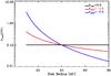 |
Fig. 1 Radial profile of the maximum grain size amax(R). Different curves represent different values of the parameter bmax as labeled but have the same amax,0 = 1 mm at 40 AU. |
3. Effect of the radial variation in the maximum grain size on disk emission
We illustrate the effects of radial changes of the maximum grain size on the disk emission at millimeter waelengths by computing a small grid of models with different grain properties. Specifically, we consider three different radial profiles of the maximum grain size amax(R) across the disk, which are obtained by varying the power-law index bmax as shown in Fig. 1. Since the spectral index of the dust opacity at mm-wavelengths β depends on the maximum grain size of the emitting dust, a radial variation in amax(R) corresponds to a radial variation in β(R).
Figure 2 shows the radial profile of β for the profiles of amax presented in Fig. 1. The black line shows the case of a maximum grain size, which is constant throughout the disk, or bmax = 0. Since amax(R) does not change with the radius, β(R) also has the same value in the disk. Red and blue lines show maximum grain size profiles, which decrease with radius, although with different power law indices as indicated in the two figures. For the dust model considered in this paper when amax ≳ 0.05 cm there is an anti-correlation between the maximum grain size and dust opacity spectral index, and this explains the general trend seen in Figs. 1 and 2. The bump seen at about 60−70 AU in the β(R) profile for the bmax = −2.5 case (blue line) is due to the increase in the dust opacity and its spectral index when amax ≈ λ/2π (see, e.g., Ricci et al. 2010a,b).
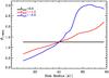 |
Fig. 2 Radial profile of β1−3 mm(R). Different curves represent different values of the parameter bmax as labeled but have the same amax,0 = 1 mm at 40 AU. |
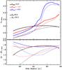 |
Fig. 3 Radial profiles of the spectral index α between 1 and 3 mm. Different curves represent different values of the parameter bmax as labeled but have the same amax,0 = 1 mm at 40 AU. The surface density profile is defined by γ = 0.5, Rtr = 20 AU, Σtr = 8 g/cm2 (solid lines), and Σtr = 30 g/cm2 (dotted lines). |
We apply the disk model described in the previous section to derive the disk surface brightness distribution at 1 and 3 mm and the radial profile of the spectral index α1−3 mm(R) for different radial profiles of the grain size distribution. To this end, we adopt the disk surface density parameters that best fit the interferometric data of CQ Tau: γ = 0.5, Rtr = 20 AU, and Σtr = 8 (see Sect. 4). We also consider a larger value for Σtr, i.e. 30 g/cm2 to investigate the impact of a larger dust opacity on our analysis.
The top panel of Fig. 3 shows the spectral index α1 − 3 mm(R). As a general trend, α1−3 mm(R) follows the profile of β(R). This is not surprising, since the difference α − β at a given radius would be equal to 2 if the dust emission at these wavelengths is optically thin and in the Rayleigh-Jeans tail of the spectrum. If either one or both of these conditions is not strictly met, then α1 − 3 mm would decrease, hence α − β < 2. The lower panel of Fig. 3 shows that this is the case at all radii for the models presented here. In particular, the innermost regions of the disk are dense enough to make the dust emission depart from the optically thin limit at these wavelengths. In the outer regions of the disk midplane, the dust temperature is cold enough to make the disk emission deviate from the Rayleigh-Jeans approximation. The combination of these two effects explains why α − β is always lower than 2 for our disks; the largest deviation corresponds to the case of the denser disks (dotted lines) because of the higher optical depths.
The models discussed in this section have been computed for a fully flared disk. If the flaring angle is smaller due to dust sedimentation, disks would be cooler and departures from Rayleigh-Jeans regime would extend to smaller radii; a simple derivation of β from α (β ~ α − 2) would result in underestimating β by large factors. In general, the disk geometry should be considered as a free parameter in the fitting procedure, unless additional constraints are available.
The examples of Fig. 3 illustrate how the radial profile of the spectral index α1−3 mm is not uniquely determined by the dust properties, but depends on the absolute values and radial dependence of the surface density profile and temperature. This shows that an accurate determination of β(R) cannot be obtained by α(R) alone. Disentangling the dependence of β on the radius from the surface density and temperature profiles can only be done by simultaneously fitting a set of spatially resolved data at different sub-mm wavelengths, as we discuss in the following sections.
4. Model fitting to the visibility data of CQ Tau
In our models, the surface density profile is defined by three parameters (γ,Rtr,Σtr; see Eq. (1)) which can vary independently. Two additional free parameters (amax,0,bmax; see Eq. (3)) describe the dust properties. All the other quantities are either fixed, or computed self-consistently, as described in Sect. 2. We assume fully flared models because they are appropriate for CQ Tau, as shown by its SED (Natta et al. 2001). We extended the procedure developed by Banzatti et al. (2011) to simultaneously fit interferometric visibilities at multiple wavelengths. A brief summary of the procedure is as follows: for each set of the disk model free parameters, we produce a theoretical image of the disk at each wavelength λi. This image is Fourier transformed and sampled at the appropriate positions on the (u,v) plane corresponding to the observed samples. We then compute the  value at each wavelength as in Banzatti et al. (2011). The global value of the χ2 for the parameter set is computed as the sum of the over the observed λi. To find the best fitting model, we searched the minimum of the
  as a function of all parameters.
For our analysis, we use the PdBI datasets at 1.3 and 2.7 mm and the VLA dataset at 7 mm presented in Banzatti et al. (2011). Data for CQ Tau at longer wavelengths do not have enough sensitivity (1.3 cm) or are dominated by ionized gas emission (3.6 cm). The SMA data at shorter wavelengths (0.87 mm) were excluded from the fit for various reasons: the dataset is very limited both in terms of the number of sampled points in the (u,v) plane and of the range of baselines probed; in addition, the fits from Banzatti et al. (2011) showed that the amplitude scale for these data may be incorrect. This latter point is very clear when looking at Fig. 4 in Banzatti et al. (2011): while the surface density normalization is consistent at the other wavelengths, the fits at 0.87 mm require a normalization larger by a factor ~2−3. This could be caused by an incorrect flux calibration of the SMA observations. As we cannot be sure of the cause for this and cannot properly correct the data, we prefer to omit them in our analysis.
 |
Fig. 4
|
Values of the best fit model parameters.
As for the disk inclination i and position angle PA (measured east of north) of the CQ Tau disk, we took the values of i = 34° and PA = 42°, as constrained from the molecular gas observations of Chapillon et al. (2008).
5. Results
The values of the best fit model parameters obtained by our analysis are listed in Table 1. For each parameter we report the 1σ confidence level intervals, following the analysis of the Δχ2 projections (see Press et al. 2007). In the same Table, we also list the values of the best fit model parameters obtained when we force the same dust properties throughout the disk (i.e. bmax = 0). The best fit model shows a decrease the maximum grain size with radius with a grain size distribution characterized by bmax ≈ −1.8 and amax,0 ≈ 0.8 cm. This corresponds to a disk populated by dust grains, which are grown to sizes larger than ≈1 cm in the inner regions (R < 40 AU) and as large as a few mm in the outer regions (see top panel in Fig. 7).
In Fig. 4 we show the projections of the χ2 hypercube on the 2D planes that include the grain size distribution parameters amax,0 and bmax and the surface density parameters, γ and Rt. The figure shows that the disk surface density profile is strongly correlated with the radial profile of the grain size distribution. More specifically, the values of γ derived, assuming constant dust opacity, bmax = 0, are systematically lower than those obtained when the radial variation in the grain size distribution is considered. We argue that this correlation between the surface density and the grain size distribution might explain some of the low values of γ derived under the assumption of constant dust opacity by modeling single wavelength millimeter-wave observations (see, e.g., Isella et al. 2009).
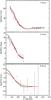 |
Fig. 5 Comparison between the data (dots) and the best-fit model predictions (solid lines) of the real part of the interferometric visibilities as a function of deprojected baseline length. The solid lines show the predicted visibilities for the best-fit model (red lines) and the best-fit model with bmax = 0 (black line). |
The comparison between the observed visibilities and the results of our model fits are shown in Fig. 5. To correct for the disk inclination, we deprojected the baselines for the assumed inclination (i = 34°) and position angle (PA = 42°) of the CQ Tau disk. The real part of the complex visibilities has then been averaged in concentric annuli of deprojected u,v distances from the disk center (in the figure, visibilities have been binned with widths of ~30, 20, and 58 kλ for data at 1.3, 3, and 7 mm, respectively). The black lines represent the best-fit model predictions obtained in the case that we assume the same dust properties throughout the disk, when bmax = 0. This model lies inside the 3σ confidence region, and although it does not correspond to the best fit, it is not rejected by our analysis.
The resulting surface density and cumulative mass radial profiles of the best fit model (first row in Table 1) are shown in the top and bottom panels of Fig. 6, respectively. These panels show disk radii up to about 80 AU. This is because the disk density at larger distances from the central star gets so low that the disk becomes optically thin to the stellar radiation, and no temperature structure can be calculated using the two-layer approximation. However, the lower panel of Fig. 6 shows that the radial profile of the cumulative mass distribution of the best fit model is already very close to being flat at ≈80 AU, indicating that the amount of disk mass lost because of this disk truncation is negligible for our analysis. The total disk gas mass, assuming a gas-to-dust mass ratio of 100, is Mg ≈ 0.006 M⊙.
When looking at the results of the model fitting and their uncertainties, one should keep in mind the strong correlation shown in Fig. 4. As a consequence, some of the model free parameters cannot vary independently within the uncertainty intervals given in Table 1, and some disk properties are better constrained than it may appear. For example, if the maximum grain size is constant with radius (bmax = 0), the surface density profile required to have a good fit of the data is characterized by γ = −0.5, Rtr = 30 AU, and Σtr = 5 g/cm2, which corresponds to a disk gas mass of Mg ~ 0.008 M⊙. This value is only 30% higher than our best fit value of 0.006 M⊙.
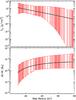 |
Fig. 6 Gas surface density (top panel) and cumulative mass (bottom panel) profiles as a function of the radius for the best-fit model. The red hatched areas indicate the allowed range of values within the 3σ uncertainty range. |
6. Discussion
The results presented in Sect. 5 indicate a moderate radial dependence of the grain sizes in the disk around CQ Tau. From the best fit values, the CQ Tau disk shows (see top panel in Fig. 7) the presence of centimeter-sized grains in the inner disk (R < 40 AU) and mm-sized grains in the outer disk (R > 40 AU). The value of β increases from ≈0.4 at about 20 AU to ≈0.8 at 80 AU and always remains lower than 1. Dust has been reprocessed and has grown in size not only in the inner denser regions but also in the outer disk. Models with constant β ~ 0.5 are consistent with the data within the 3σ confidence interval.
The radial dependence of the dust properties in the CQ Tau disk obtained in this paper confirms the suggestion of Banzatti et al. (2011) that the inner regions of the CQ Tau disk contain grains larger than those in the outer regions. Unlike the analysis presented here, they separately fitted each dataset from 0.87 mm to 7 mm using a two-layer disk model with a radial constant dust opacity distribution and adopted a power law Σ(R) = Σ0(R/R0)p profile for the surface density distribution. They obtained a variation in the fitted power-law surface density distribution with the slope p which increases with wavelength from ≈0 at 1.3 mm to ≈0.5 at 7 mm. Assuming that the unphysical variation of the surface density profile of the disk is due to radial variations in the dust opacity spectral index β (Isella et al. 2010), they concluded that β(R) must increase from ~0.0 in the inner disk to β ~ 1.4 at R ≈ 63 AU. Our analysis, based on models that allow for radial variation in β, favors slightly lower values of β in the outer disk. We think that this difference is likely due to the weight that the two techniques give to the observations at the various wavelengths. The approach used by Isella et al. (2010) gives the same weight to the results obtained at different wavelengths, while the global fit adopted here weights each observation with its own uncertainty. It should also be noted that the disk models themselves are slightly different in Banzatti et al. (2011), where a power law Σ(r) profile was adopted. The quality of the datasets available for CQ Tau does not warrant an extensive comparison of the two methods, which should be performed as soon as better datasets are available.
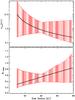 |
Fig. 7 Maximum grain size (top panel) and slope of the millimeter dust opacity (bottom panel) as function of the radius for the best-fit model. The red hatched areas indicate the allowed range of values within the 3σ uncertainty range. |
A radial dependence of β from lower to higher values for increasing radii has been found in all disks analyzed so far. Guilloteau et al. (2011) characterized the dust radial distribution in a sample of 20 disks in the Taurus-Auriga star-forming region by combining observations at 1.3 and 3 mm with the IRAM PdBI interferometer. Unlike this study, they fitted the data with parametric disk models and found a radial dependence of β, which appears to typically increase from low values (~0−0.5) within ~50−100 AU from the central star to about 1.5−2 at the disk outermost regions. Pérez et al. (2012) investigated the radial variation in the dust opacity across the AS 209 circumstellar disk by combining spatially resolved observations from sub-millimeter to centimeter wavelengths; they used a two-layer disk model similar to the one described in this paper and followed the procedure outlined in Isella et al. (2010) and Banzatti et al. (2011). Their results indicate that β(R) increases from β < 0.5 at ≈20 AU to β > 1.5 for R ≳ 80 AU.
This general trend of decreasing maximum grain size with increasing radius is predicted by theoretical models of dust evolution in circumstellar gasous disks. According to simple theoretical considerations, the efficiency of the radial drift of solid particles depends on their coupling with the gas and large grains are expected to drift inward more rapidly than small grains (Whipple 1972; Weidenschilling 1977). Hence, one naturally expects large grains in the inner region and small grains in the outer regions. If this drag is as efficient as the laminar theory predicts, dust particles of few mm in size would be removed from the outer disk in a much shorter timescale than the typical age of protoplanetary disks of few million years (Brauer et al. 2007). Recent dust evolution models, which consider the effects of radial drift, turbulent mixing, coagulation, and fragmentation, have been performed by Brauer et al. (2008) and further expanded by Birnstiel et al. (2010a) to include the viscous evolution of the gas disk. Their models predict a radial dependence of the grain growth level that is a function of the local physical conditions in the disk (temperature, density, strength of the turbulence, and fragmentation velocity). However, they show that the combination of radial drift and fragmentation is a strong limitation to particle growth and represents an obstacle for the formation of planetesimals (known as the fragmentation barrier). Assuming that the radial drift is halted by some unknown physical mechanism, Birnstiel et al. (2010b) compared the predictions of dust evolution models, including grain coagulation and fragmentation, with the results of sub-mm observations of disks (Ricci et al. 2010a,b). In most of the adopted models, they predicted steady-state grain size distributions that lead to dust opacity index β(R) that increases with radius, which agree with our finding.
Within the general trend described above, models predict that the combined effect of the many physical processes involved should produce grains with different properties in different disks. This seems to be confirmed by the few observational results obtained so far, which seem to indicate differences in the values of β in the outer regions of different disks. In particular, CQ Tau seems to have very evolved grains also in the outer disk. However, one should keep in mind that the CQ Tau disk is small compared to others and that our results are affected by large uncertainties.
7. Summary and conclusions
We have attempted to constrain the radial distribution of the grain size distribution in the disk around CQ Tau. We propose a new method that is based on disk models that include the radial variations in the grain properties in a self-consistent way. These models are used to simultaneously fit a set of interferometric observations at different wavelengths and allow us to constrain at the same time the disk structure and the dust properties.
In CQ Tau, we find that the similarity solution for the viscous evolution of Keplerian disks (Lynden-Bell & Pringle 1974) provides a good fit to the multiwavelength continuum observations at 1.3, 2.7, and 7 mm. Although a model with a constant grain size distribution across the disk is still marginally consistent with the interferometric data, the model which best fits the data requires a radial dependence of the dust opacity. The resulting maximum grain size distribution is found to decrease with the radius from a few cm at ~20−40 AU from the star to a few mm further away from the star. Although the trend is similar to the prediction of dust grain evolution models, which include coagulation and fragmentation (Birnstiel et al. 2010b), it seems that grains are more evolved in the outer disk than in other objects investigated recently with other methods. This may be due to the large uncertainties present in all cases but may also reflect the relatively small size of the CQ Tau disk.
The results show that our self-consistent approach can be successfully applied to the analysis of mm interferometric data. The investigation of radial variations in the dust properties is still strongly limited by the relatively poor angular resolution and sensitivity of the current sub-mm facilities. Observations with higher angular resolution and sensitivity are needed to place more stringent constraints on the radial variation in the dust opacity. For these purposes, the ALMA and VLA arrays will play a crucial role in the near future.
radius at which the mass flow through the disk changes direction, so that the resulting mass flow for R < Rtr is directed inward (disk accretion) and outward for R > Rtr (disk expansion).
Acknowledgments
We thank Tillman Birnstiel for many useful discussions on grain growth in circumstellar disks. This research was partly supported by the Italian Space Agency (ASI) as part of the ASI-INAF agreement number I/005/11/0. A.I. acknowledge support from NSF award AST-1109334.
References
- Andrews, S. M., & Williams, J. P. 2005, ApJ, 631, 1134 [NASA ADS] [CrossRef] [Google Scholar]
- Armitage, P. J. 2011, ARA&A, 49, 195 [NASA ADS] [CrossRef] [EDP Sciences] [Google Scholar]
- Banzatti, A., Testi, L., Isella, A., et al. 2011, A&A, 525, A12 [NASA ADS] [CrossRef] [EDP Sciences] [Google Scholar]
- Beckwith, S. V. W., & Sargent, A. I. 1991, ApJ, 381, 250 [NASA ADS] [CrossRef] [Google Scholar]
- Birnstiel, T., Dullemond, C. P., & Brauer, F. 2010a, A&A, 513, 79 [Google Scholar]
- Birnstiel, T., Ricci, L., Trotta, F., et al. 2010b, A&A, 516, 14 [Google Scholar]
- Boehler, Y., Dutrey, A., Guilloteau, S., & Pietu, V. 2013, MNRAS, 431, 1573 [NASA ADS] [CrossRef] [Google Scholar]
- Borucki, W. J., Koch, D. G., Basri, G., Batalha, N., et al. 2011, ApJ, 736, 19 [NASA ADS] [CrossRef] [Google Scholar]
- Brauer, F., Dullemond, C. P., Johansen, A., et al. 2007, A&A, 469, 1169 [NASA ADS] [CrossRef] [EDP Sciences] [Google Scholar]
- Brauer, F., Dullemond, C. P., & Henning, Th. 2008, A&A, 480, 859 [NASA ADS] [CrossRef] [EDP Sciences] [Google Scholar]
- Bruggeman, D. A. G. 1935, Ann. Phys. Leipzig, 24, 636 [NASA ADS] [CrossRef] [Google Scholar]
- Chapillon, E., Guilloteau, S., Dutrey, A., & Pietu, V. 2008, A&A, 488, 565 [NASA ADS] [CrossRef] [EDP Sciences] [Google Scholar]
- Chiang, E. I., & Goldreich, P. 1997, ApJ, 490, 368 [NASA ADS] [CrossRef] [Google Scholar]
- Chiang, E. I., Joung, M. K., Creech-Eakman, M. J., et al. 2001, ApJ, 547, 1077 [NASA ADS] [CrossRef] [Google Scholar]
- Draine, B. T. 2006, ApJ, 636, 1114 [NASA ADS] [CrossRef] [Google Scholar]
- Dullemond, C. P., & Dominik, C. 2004, A&A, 421, 1075 [NASA ADS] [CrossRef] [EDP Sciences] [Google Scholar]
- Dullemond, C. P., Dominik, C., & Natta, A. 2001, ApJ, 560, 957 [NASA ADS] [CrossRef] [Google Scholar]
- Guilloteau, S., Dutrey, A., Pietu, V., & Boehler, Y. 2011, A&A, 529, 105 [Google Scholar]
- Hartmann, L., Calvet, N., Gullbring, E., & D’Alessio, P. 1998, ApJ, 495, 385H [NASA ADS] [CrossRef] [Google Scholar]
- Isella, A., Carpenter, J. M., & Sargent, A. I. 2009, ApJ, 701, 260 [NASA ADS] [CrossRef] [Google Scholar]
- Isella, A., Carpenter, J. M., & Sargent, A. I. 2010, ApJ, 714, 1746 [NASA ADS] [CrossRef] [Google Scholar]
- Johansen, A., & Klahr, H. 2005, ApJ, 634, 1353J [NASA ADS] [CrossRef] [Google Scholar]
- Lissauer, J. J. 1993, ARA&A, 31, 129 [NASA ADS] [CrossRef] [Google Scholar]
- Lommen, D., Wright, C. M., Maddison, S. T., et al. 2007, A&A, 462, 211 [NASA ADS] [CrossRef] [EDP Sciences] [Google Scholar]
- Lommen, D., Maddison, S. T., Wright, C. M., et al. 2009, A&A, 495, 869 [NASA ADS] [CrossRef] [EDP Sciences] [Google Scholar]
- Lynden-Bell, D., & Pringle, J. E. 1974, MNRAS, 168, 603 [NASA ADS] [CrossRef] [Google Scholar]
- Natta, A., Grinin, V., & Mannings, V. 2000, Protostars and Planets IV (Tucson: University of Arizona Press), 559 [Google Scholar]
- Natta, A., Prusti, T., Neri, R., et al. 2001, A&A, 371, 186 [NASA ADS] [CrossRef] [EDP Sciences] [Google Scholar]
- Natta, A., Testi, L., Neri, R., Shepherd, D. S., & Wilner, D. J. 2004, A&A, 416, 179 [NASA ADS] [CrossRef] [EDP Sciences] [Google Scholar]
- Natta, A., Testi, L., Calvet, N., et al. 2007, in Protostars & Planets V, eds. B. Reipurth, D. Jewitt, & K. Keil (Tucson: University of Arizona Press), 783 [Google Scholar]
- Perez, L. M., Carpenter, J. M., Chandler, C. J., et al. 2012, ApJ, 760, L17 [NASA ADS] [CrossRef] [Google Scholar]
- Perryman, M. A. C., Lindegren, L., Kovalevsky, J., et al. 1997, A&A, 323, L49 [NASA ADS] [Google Scholar]
- Press, W. H., Teukolsky, S. A., Vetterling, W. T., & Flannery, B. P. 2007, Numerical Recipes: The Art of Scientific Computing, Third Edition (New York: Cambridge University Press) [Google Scholar]
- Ricci, L., Testi, L., Natta, A., et al. 2010a, A&A, 512, 15 [Google Scholar]
- Ricci, L., Testi, L., Natta, A., & Brooks, K. J. 2010b, A&A, 521, 66 [Google Scholar]
- Ricci, L., Mann, R. K., Testi, L., et al. 2011, A&A, 525, 81 [Google Scholar]
- Rodmann, J., Henning, T., Chandler, C. J., Mundy, L. G., & Wilner, D. J. 2006, A&A, 446, 211 [NASA ADS] [CrossRef] [EDP Sciences] [Google Scholar]
- Semenov, D., Henning, T., Helling, C., Ilgner, M., & Sedlmayr, E. 2003, A&A, 410, 611 [NASA ADS] [CrossRef] [EDP Sciences] [Google Scholar]
- Shakura, N. I., & Syunyaev, R. A. 1973, A&A, 24, 337 [NASA ADS] [Google Scholar]
- Testi, L., Natta, A., Shepherd, D. S., & Wilner, D. J. 2001, ApJ, 554, 1087 [Google Scholar]
- Testi, L., Natta, A., Shepherd, D. S., & Wilner, D. J. 2003, A&A, 403, 323 [NASA ADS] [CrossRef] [EDP Sciences] [Google Scholar]
- Ubach, C., Maddison, S. T., Wright, C. M., et al. 2012, MNRAS, 425, 3137 [NASA ADS] [CrossRef] [Google Scholar]
- Warren, S. G. 1984, Appl. Opt., 23, 1206 [NASA ADS] [CrossRef] [PubMed] [Google Scholar]
- Weidenschilling, S. J. 1977, MNRAS, 180, 57 [NASA ADS] [CrossRef] [Google Scholar]
- Weingartner, J. C., & Draine, B. T. 2001, ApJ, 548, 296 [NASA ADS] [CrossRef] [Google Scholar]
- Whipple, F. L. 1972, in From Plasma to Planet (New York: Wiley Interscience Division), 211 [Google Scholar]
- Wilner, D. J., Ho, P. T. P., Kastner, J. H., & Rodríguez, L. F. 2000, ApJ, 534, L101 [NASA ADS] [CrossRef] [PubMed] [Google Scholar]
- Wilner, D. J., D’Alessio, P., Calvet, N., et al. 2005, ApJ, 626, L109 [NASA ADS] [CrossRef] [Google Scholar]
- Zubko, V. G., Mennella, V., Colangeli, L., & Bussoletti, E. 1996, MNRAS, 282, 1321 [NASA ADS] [CrossRef] [Google Scholar]
All Tables
All Figures
|
Fig. 1 Radial profile of the maximum grain size amax(R). Different curves represent different values of the parameter bmax as labeled but have the same amax,0 = 1 mm at 40 AU. |
| In the text | |
|
Fig. 2 Radial profile of β1−3 mm(R). Different curves represent different values of the parameter bmax as labeled but have the same amax,0 = 1 mm at 40 AU. |
| In the text | |
|
Fig. 3 Radial profiles of the spectral index α between 1 and 3 mm. Different curves represent different values of the parameter bmax as labeled but have the same amax,0 = 1 mm at 40 AU. The surface density profile is defined by γ = 0.5, Rtr = 20 AU, Σtr = 8 g/cm2 (solid lines), and Σtr = 30 g/cm2 (dotted lines). |
| In the text | |
|
Fig. 4
|
| In the text | |
|
Fig. 5 Comparison between the data (dots) and the best-fit model predictions (solid lines) of the real part of the interferometric visibilities as a function of deprojected baseline length. The solid lines show the predicted visibilities for the best-fit model (red lines) and the best-fit model with bmax = 0 (black line). |
| In the text | |
|
Fig. 6 Gas surface density (top panel) and cumulative mass (bottom panel) profiles as a function of the radius for the best-fit model. The red hatched areas indicate the allowed range of values within the 3σ uncertainty range. |
| In the text | |
|
Fig. 7 Maximum grain size (top panel) and slope of the millimeter dust opacity (bottom panel) as function of the radius for the best-fit model. The red hatched areas indicate the allowed range of values within the 3σ uncertainty range. |
| In the text | |
Current usage metrics show cumulative count of Article Views (full-text article views including HTML views, PDF and ePub downloads, according to the available data) and Abstracts Views on Vision4Press platform.
Data correspond to usage on the plateform after 2015. The current usage metrics is available 48-96 hours after online publication and is updated daily on week days.
Initial download of the metrics may take a while.