| Issue |
A&A
Volume 558, October 2013
|
|
|---|---|---|
| Article Number | A114 | |
| Number of page(s) | 11 | |
| Section | Stellar structure and evolution | |
| DOI | https://doi.org/10.1051/0004-6361/201321866 | |
| Published online | 15 October 2013 | |
Accurate determination of accretion and photospheric parameters in young stellar objects: The case of two candidate old disks in the Orion Nebula Cluster ⋆
1
European Southern Observatory, Karl Schwarzschild Str. 2, 85748
Garching, Germany
e-mail: cmanara@eso.org
2
European Space Agency, Keplerlaan 1, 2200 AG
Noordwijk, The
Netherlands
3
INAF - Osservatorio Astrofisico di Arcetri,
Largo E. Fermi 5, 50125
Firenze,
Italy
4
School of Cosmic Physics, Dublin Institute for Advanced
Studies, 31 Fitzwilliam Place,
2
Dublin,
Ireland
5
California Institute of Technology, 1200 East California Boulervard, Pasadena, CA
91125,
USA
6
Space Telescope Science Institute, 3700 San Martin Dr., Baltimore, MD
21218,
USA
7
Excellence Cluster Universe, Boltzmannstr. 2, 85748
Garching,
Germany
Received:
9
May
2013
Accepted:
26
July
2013
Context. Current planet formation models are largely based on the observational constraint that protoplanetary disks have a lifetime of ~3 Myr. Recent studies, however, report the existence of pre-main-sequence stars with signatures of accretion (strictly connected with the presence of circumstellar disks) and photometrically determined ages of 30 Myr or more.
Aims. Here, we present a spectroscopic study of two major age outliers in the Orion Nebula Cluster. We use broadband, intermediate resolution VLT/X-shooter spectra combined with an accurate method to determine the stellar parameters and the related age of the targets to confirm their peculiar age estimates and the presence of ongoing accretion.
Methods. The analysis is based on a multicomponent fitting technique, which derives simultaneously spectral type, extinction, and accretion properties of the objects. With this method, we confirm and quantify the ongoing accretion. From the photospheric parameters of the stars, we derive their position on the H-R diagram and the age given by evolutionary models. With other age indicators like the lithium-equivalent width, we estimate the age of the objects with high accuracy.
Results. Our study shows that the two objects analyzed are not older than the typical population of the Orion Nebula Cluster. While photometric determination of the photospheric parameters are an accurate method to estimate the parameters of the bulk of young stellar populations, our results show that those of individual objects with high accretion rates and extinction may be affected by large uncertainties. Broadband spectroscopic determinations should thus be used to confirm the nature of individual objects.
Conclusions. The analysis carried out shows that this method allows us to obtain an accurate determination of the photospheric parameters of accreting young stellar objects in any nearby star-forming region. We suggest that our detailed, broadband spectroscopy method should be used to derive accurate properties of candidate old and accreting young stellar objects in star-forming regions. We also discuss how a similarly accurate determination of stellar properties can be obtained through a combination of photometric and spectroscopic data.
Key words: stars: pre-main sequence / stars: variables: T Tauri, Herbig Ae/Be / stars: formation
© ESO, 2013
1. Introduction
The formation of planetary systems is strongly connected to the presence, structure, and evolution of protoplanetary disks in which they are born. In particular, the timescale of disk survival sets an upper limit on the timescale of planet formation, becoming a stringent constraint for planet formation theories (Haisch et al. 2001; Wolf et al. 2012). As the observed timescale for the evolution of the inner disk around pre-main sequence (PMS) stars is on the order of a few Myr (e.g., Williams & Cieza 2011), all models proposed to explain the gas giant planet formation (core accretion, gravitational instability) are generally constrained to agree with a disk lifetime of much less than 10 Myr.
Parameters available in the literature for the objects analyzed in this work.
Observations of nearby young clusters (age ≲ 3 Myr) show the presence of few outliers with derived isochronal ages of more than 10 Myr. For example, this is found in the Orion Nebula Cluster (ONC; Da Rio et al. 2010a, 2012) and in Taurus (White & Hillenbrand 2005). The age of the objects is derived from their position on the H-R diagram (HRD) and thus subject to several uncertainties, which are either observational (e.g., spectral type, extinction), intrinsic to the targets (e.g., strong variability, edge-on disk presence, Huélamo et al. 2010), or related to the assumed evolutionary models (e.g., Da Rio et al. 2010b; Baraffe & Chabrier 2010; Barentsen et al. 2011). On the other hand, observations of far (d > 1 kpc) and extragalactic more massive clusters revealed the presence of a large population of accreting objects older (ages > 30 Myr) than the typical ages assumed for the cluster (~3−5 Myr). Examples of these findings are the studies of NGC 3603 (Beccari et al. 2010), NGC 6823 (Riaz et al. 2012) and of various regions of the Magellanic Clouds (De Marchi et al. 2010, 2011; Spezzi et al. 2012). Observations in these clusters are dominated by solar- and intermediate-mass stars, for which the age determination is subject to the same uncertainties as for nearby clusters, but also to other uncertainties: For example, the age of these more massive targets is more sensitive to assumptions on the birthline (Hartmann 2003).
These findings challenge the present understanding of protoplanetary disk evolution and can imply a entirely new scenario for the planet formation mechanism. On one side, the existence of one or few older disks in young regions does not change the aforementioned disk evolution timescales but represents a great benchmark of a possible new class of objects, where planet formation is happening on longer timescales. In contrast, the presence of a large population of older objects, representing a significant fraction of the total cluster members, could imply a totally different disk evolution scenario in those environments.
We thus want to verify the existence and the nature of older and still active protoplanetary disks in nearby regions. For this reason we have developed a spectroscopic method, which allows us to consistently and accurately determine the stellar and accretion properties of the targeted objects. Here, we present a pilot study carried out with the ESO/VLT X-shooter spectrograph targeting two major age outliers with strong accretion activity in the ONC. This is an ideal region for this study, given its young mean age (~2.2 Myr, Reggiani et al. 2011), its vicinity (d = 414 pc, Menten et al. 2007), the large number of objects (more than 2000, Da Rio et al. 2010a), and the large number of previous studies (e.g., Hillenbrand 1997; Da Rio et al. 2010a, 2012; Megeath et al. 2012; Robberto et al. 2013). Our objectives are therefore a) to verify the previously derived isochronal ages of these two objects by using different and more accurate age indicators and b) to assess the presence of an active disk with ongoing accretion.
The structure of the paper is the following. In Sect. 2, we report the targets selection criteria, the observation strategy, and the data reduction procedure. In Sect. 3, we describe the procedure adopted to derive the stellar parameters of the objects; and in Sect. 4, we report our results. In Sect. 5, we discuss the implications of our findings. Finally, we summarize our conclusions in Sect. 6.
2. Sample, observations, and data reduction
2.1. Targets selection and description
We have selected the two older PMS candidates from the sample of the Hubble Space Telescope (HST) Treasury Program on the ONC (Robberto et al. 2013). Our selection criteria were as follows: clear indications of ongoing accretion and of the presence of a protoplanetary disk; an estimated isochronal age much larger than the mean age of the cluster, i.e. ≳30 Myr; a location well outside the bright central region of the nebula to avoid intense background contamination, which corresponds to a distance from θ1 Orionis C larger than 5′(~0.7 pc); and low foreground extinction (AV ≲ 2 mag). To find the best candidates, we have combined HST broadband data (Robberto et al. 2013) with narrow-band photometric and spectroscopic data (Hillenbrand 1997; Stassun et al. 1999; Da Rio et al. 2010a, 2012) with mid-infrared photometric data (Megeath et al. 2012). According to Da Rio et al. (2010a, 2012), the total number of PMS star candidates in the ONC field with a derived isochronal age ≳ 10 Myr, which is derived using various evolutionary models (D’Antona & Mazzitelli 1994; Siess et al. 2000; Palla & Stahler 1999; Baraffe et al. 1998), is ~165 including both accreting and nonaccreting targets, which corresponds to ~10% of the total population. Among these, ~90 objects (~5%) have ages ≳30 Myr. The presence of ongoing accretion has been estimated through the Hα line equivalent width (EWHα) reported in Da Rio et al. (2010a). We use a threshold value of EWHα > 20 Å, which implies non negligible mass accretion rates (Ṁacc ≳ 10-9 M⊙/yr). This is a high threshold that leads to select stronger accretors. Following White & Basri (2003) and Manara et al. (2013), objects with EWHα < 20 Å can still be accretors but with a lower accretion rate. The available Spitzer photometry (Megeath et al. 2012) has been used to confirm the presence of an optically thick circumstellar disk, which is already suggested by the strong Hα emission. This is performed by looking at the spectral energy distribution (SED) of the targets to see clear excess with respect to the photospheric emission in the mid-infrared wavelength range. Among the objects with isochronal age ≳10 Myr, there are ten objects (<1%) showing very strong Hα excess, or EWHα > 20 Å. Very striking, two PMS star candidates, each with an isochronal age ≳ 30 Myr, have clear indications of Hα excess and the presence of the disk from IR photometry. These two extreme cases of older-PMS star candidates are selected for this work.
The two targets selected are OM1186 and OM3125, and we report their principal parameters available from Da Rio et al. (2010a, and reference therein) in Table 1. Both targets are located on the HRD almost on the main sequence, as we show in Fig. 1, where the position of these sources is reported using green stars. We also plot the position of other PMS star candidates in the ONC field, as shown with blue circles if their EWHα < 20 Å and with red diamonds if EWHα ≥ 20 Å. Their position on the HRD clearly indicates that they have an isochronal age much larger than the bulk of the ONC population with ages between ~60 Myr and ~90 Myr for OM1186, according to different evolutionary tracks, and between ~25 Myr and ~70 Myr for OM3125. The spectral type (SpT) of the two targets has been determined in Hillenbrand (1997) to be K5 for OM1186 and G8-K0 for OM3125.
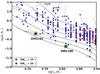 |
Fig. 1 H-R diagram of the ONC from Da Rio et al. (2012) with green stars showing the positions of the two targets of this study. The overplotted evolutionary tracks are from D’Antona & Mazzitelli (1994). We plot (from top to bottom) the 0.3, 1, 3, 10, 30, and 100 Myr isochrones. |
2.2. Observations and data reduction
Observations with the ESO/VLT X-shooter spectrograph have been carried out in service mode between February and March 2012 (ESO/DDT program 288.C-5038, PI Manara). This instrument covers the wavelength range between ~300 nm and ~2500 nm simultaneously, dividing the spectrum in three arms – namely, the UVB arm in the region λλ ~ 300−550 nm, the VIS arm between λλ ~ 550−1050 nm, and NIR from λ ~ 1050 nm to λ ~ 2500 nm (Vernet et al. 2011). The targets have been observed in slit-nodding mode to have a good sky subtraction in the NIR arm. For both targets we used the same slit widths (0.5′′ in the UVB arm and 0.4′′ in the other two arms) and the same exposure times (300 s × 4 in all three arms) to ensure the highest possible resolution of the observations (R = 9100, 17 400, and 10500 in the UVB, VIS, and NIR arms, respectively) and enough S/N in the UVB arm. The readout mode used in both cases was “100,1 × 1,hg”. The seeing conditions of the observatory during the observations were 1′′ for OM1186 and 0.95′′ for OM3125.
Data reduction has been carried out using the version 1.3.7 of the X-shooter pipeline (Modigliani et al. 2010), which is run through the EsoRex tool. The spectra were reduced independently for the three spectrograph arms. The pipeline with the standard reduction steps (i.e., bias or dark subtraction, flat-fielding, spectrum extraction, wavelength calibration, and sky subtraction) also considers the flexure compensation and the instrumental profile. Particular care has been paid to the flux calibration and telluric removal of the spectra. Flux calibration has been carried out within the pipeline and then compared with the available photometry (Robberto et al. 2013) to correct for possible slit losses. We have also checked the conjunctions between the three arms. The overall final agreement is very good. Telluric removal has been carried out using the standard telluric spectra that have been provided as part of the X-shooter calibration plan on each night of observations. The correction has been accomplished using the IRAF1 task telluric, using the procedure explained in Alcalá et al. (2013).
3. Method
The determination of SpT and stellar properties in accreting young stellar objects (YSOs) is not trivial for a variety of reasons. First, YSOs are usually still embedded in their parental molecular cloud, which originates differential reddening effects in the region. This with the presence of a circumstellar disk surrounding the star can modify the actual value of the extinction (AV) on the central YSO from one object to another. Second, YSOs may still be accreting material from the protoplanetary disk on the central star. This process affects the observed spectrum of a YSO – producing excess continuum emission in the blue part of the spectrum, veiling of the photospheric absorption features at all optical wavelengths and adding several emission lines (e.g., Hartmann et al. 1998). The two processes modify the observed spectrum in opposite ways: extinction toward the central object suppresses the blue part of the spectrum, making the central object appear redder and thus colder, while accretion produces an excess continuum emission, which is stronger in the blue part of the spectrum, making the observed central object look hotter.
For these reasons, SpT, AV, and accretion
properties should be considered together in the analysis of these YSOs. Here, we present the
minimum  method that we
use to determine SpT, AV, and the accretion
luminosity (Lacc) simultaneously. With this procedure, we are
able to estimate L∗, which is used to derive
M∗, the age of the target using different evolutionary models,
and the mass accretion rate (Ṁacc). Finally, we determine the
surface gravity (log g) for the input object by comparison to synthetic
spectra.
method that we
use to determine SpT, AV, and the accretion
luminosity (Lacc) simultaneously. With this procedure, we are
able to estimate L∗, which is used to derive
M∗, the age of the target using different evolutionary models,
and the mass accretion rate (Ṁacc). Finally, we determine the
surface gravity (log g) for the input object by comparison to synthetic
spectra.
3.1. Parameters of the multicomponent fit
To fit the optical spectrum of our objects, we consider three components: a set of photospheric templates, which are used to determine the SpT and therefore the effective temperature (Teff) of the input spectrum; different values of the extinction and a reddening law to obtain AV; and a set of models, which describe the accretion spectrum that we use to derive Lacc.
Photospheric templates. The set of photospheric templates is obtained from the one collected in Manara et al. (2013). This is a sample of 24 well-characterized X-shooter spectra of nonaccreting (Class III) YSOs which are representative of objects of SpT classes from late K to M. We extend this grid with two new X-shooter observations of nonaccreting YSOs from the ESO programs 089.C-0840 and 090.C-0050 (PI Manara): one object with SpT G4 and the other one with SpT K2. In total, our photospheric templates grid consists of 26 nonaccreting YSOs with SpT between G4 and M9.5. We use Class III YSOs as a photospheric template, because synthetic spectra or field dwarfs spectra would be inaccurate for this analysis for the following reasons. First, YSOs are highly active, and their photosphere is strongly modified by this chromospheric activity in both the continuum and the line emission (e.g., Ingleby et al. 2011; Manara et al. 2013). Second, field dwarf stars have a different surface gravity with respect to PMS stars, which are sub-giants. Using spectra of nonaccreting YSOs as templates mitigates these problems.
Extinction. In the analysis we consider values of AV in the range [0−10] mag with steps of 0.1 mag in the range AV = [0−3] mag and 0.5 mag at higher values of AV. This includes all the possible typical values of AV for nonembedded objects in this region (e.g., Da Rio et al. 2010a, 2012). The reddening law adopted in this work is from Cardelli et al. (1989) with RV = 3.1, which is appropriate for the ONC region (Da Rio et al. 2010a).
Accretion spectrum. To determine the excess emission due to accretion and thus Lacc, we use a grid of isothermal hydrogen slab models, which has already been used and proven to be adequate for this analysis (e.g., Valenti et al. 1993; Herczeg & Hillenbrand 2008; Rigliaco et al. 2012; Alcalá et al. 2013). We describe the emission due to accretion with the slab model to have a good description of the shape of this excess and to correct for the emission arising in the spectral region at wavelengths shorter than the minimum wavelengths covered by the X-shooter spectra at λ ≲ 330 nm. In these models, we assume local thermodynamic equilibrium (LTE) conditions, and we include both the H and H− emission. Each model is described by three parameters: the electron temperature (Tslab), the electron density (ne), and the optical depth at λ = 300 nm (τ), which is related to the slab length. The Lacc is given by the total luminosity emitted by the slab. The grid of slab models adopted covers the typical values for the three parameters: Tslab are selected in the range from 5000 to 11 000 K, ne varies from 1011 to 1016 cm-3, and τ has values between 0.01 and 5.
Additional parameters. In addition to the five parameters just introduced – namely, the photospheric template, AV, and the three slab model parameters (Tslab, ne, τ), there is the need to also include two normalization constant parameters: one for the photospheric template (Kphot) and one for the slab model (Kslab). The first rescales the emitted flux of the photospheric template to the correct distance and radius of the input target, while the latter converts the slab emission flux as it would have been emitted at the stellar surface by a region with the area given by the slab parameters.
3.2. Determination of the best fit
To consider the three components (SpT, AV,
Lacc) together, we develop a Python procedure, which
determines the model that best fits the observed spectrum. We calculate a likelihood
function for each point of the model grid, which can be compared to a
χ2 distribution, by comparing the observed and model spectra
in a number of spectral features. These are chosen in order to consider both the region
around the Balmer jump, where the emitted flux mostly originates in the accretion shock,
and regions at longer wavelengths, where the photospheric emission dominates the observed
spectrum. The form of this function that is addressed as
function is
the following: ![\begin{equation} \chi^2_{\rm like} = \sum_{\rm features} \left[\frac{ f_{\rm obs} - f_{\rm mod} }{\sigma _{\rm obs}} \right]^2 , \label{eq::chi2} \end{equation}](/articles/aa/full_html/2013/10/aa21866-13/aa21866-13-eq50.png) (1)where
f is the value of the measured feature, obs refers to measurements
operated on the observed spectrum, mod refers to those on the model spectrum, and
σobs is the error on the value of the feature in the
observed spectrum. The features considered here are the Balmer jump ratio, defined as the
ratio between the flux at ~360 nm and ~400 nm; the slope of the Balmer
continuum between ~335 nm and ~360 nm; the slope of the Paschen
continuum between ~400 nm and ~475 nm; the value of the Balmer continuum
at ~360 nm; that of the Paschen continuum at ~460 nm; and the value of
the continuum in different bands at ~710 nm. The exact wavelength ranges of these
features are reported in Table 2. The best fit
model is determined by minimizing the distribution.
The exact value of the best fit is not
reported, because this value itself should not be considered as an accurate estimate of
the goodness of the fit. Whereas a fit with a value of
which is much
larger than the minimum leads to a very poor fit of the observed spectrum, this function
is not a proper χ2, given that it considers only the errors on
the observed spectrum and only some regions in the spectrum.
(1)where
f is the value of the measured feature, obs refers to measurements
operated on the observed spectrum, mod refers to those on the model spectrum, and
σobs is the error on the value of the feature in the
observed spectrum. The features considered here are the Balmer jump ratio, defined as the
ratio between the flux at ~360 nm and ~400 nm; the slope of the Balmer
continuum between ~335 nm and ~360 nm; the slope of the Paschen
continuum between ~400 nm and ~475 nm; the value of the Balmer continuum
at ~360 nm; that of the Paschen continuum at ~460 nm; and the value of
the continuum in different bands at ~710 nm. The exact wavelength ranges of these
features are reported in Table 2. The best fit
model is determined by minimizing the distribution.
The exact value of the best fit is not
reported, because this value itself should not be considered as an accurate estimate of
the goodness of the fit. Whereas a fit with a value of
which is much
larger than the minimum leads to a very poor fit of the observed spectrum, this function
is not a proper χ2, given that it considers only the errors on
the observed spectrum and only some regions in the spectrum.
Spectral features used to calculate the best-fit in our multicomponent fit procedure.
The procedure is as follows. For each photospheric template we deredden the observed
spectrum with increasing values of AV.
Considering each slab model, we then determine the value of the two normalization
constants Kphot and Kslab for
every value of AV. This is done matching the
normalized sum of the photosphere and the slab model to the observed dereddened spectrum
at λ ~ 360 nm and at λ ~ 710 nm. After
that, we calculate the value using
Eq. (1). This is done for each point of the
grid (SpT, AV, slab parameters). After the
iteration on each point of the grid terminates, we find the minimum value of the
and the
correspondent values of the best fit parameters (SpT,
AV, slab parameters,
Kphot, Kslab).
We also derive the uncertainties on these two parameters and thus on
Lacc from the  distribution
with respect to the SpT of the photospheric templates and the different values of
AV. Indeed, these are the main sources of
uncertainty in the determination of Lacc, which is a
measurement of the excess emission with respect to photospheric emission due to accretion.
Most of the accretion excess (≳70%) is emitted in regions covered by our X-shooter spectra
and originates mostly in the wavelength range of λ ~ 330–1000
nm, while most of the excess emission at longer wavelengths is due to disk emission and is
not considered in our analysis. To derive the total excess due to accretion, we need a
bolometric correction for the emission at wavelengths shorter than those in the X-shooter
range at λ ≲ 330 nm. This is calculated with the best fit slab model. Our
analysis of the slab models lead to the conclusion that this contribution accounts for
less than 30% of the excess emission and that the shape of this emission is well
constrained by the Balmer continuum slope. Different slab model parameters with reasonable
Balmer continuum slopes that would imply similarly good fits as the best one would lead to
values of Lacc always within 10% of each other, as it has also
been pointed out by Rigliaco et al. (2012).
Therefore, once SpT and AV are constrained,
the results with different slab parameters are similar. With our procedure, we can very
well constrain all the parameters. Typically, the solutions with
values closer
to the best-fit are those within one spectral subclass of difference in the photospheric
template at ±0.1−0.2 mag in extinction values and with differences of
Lacc of less than ~10%. Other sources of
uncertainty on the estimate of Lacc are the noise in the
observed and template spectra, the uncertainties in the distances of the target, and the
uncertainty given by the exclusion of emission lines in the estimate of the excess
emission (see e.g., Herczeg & Hillenbrand
2008; Rigliaco et al. 2012; Alcalá et al. 2013). Typical errors altogether on
estimates of Lacc with our method are of 0.2−0.3 dex.
distribution
with respect to the SpT of the photospheric templates and the different values of
AV. Indeed, these are the main sources of
uncertainty in the determination of Lacc, which is a
measurement of the excess emission with respect to photospheric emission due to accretion.
Most of the accretion excess (≳70%) is emitted in regions covered by our X-shooter spectra
and originates mostly in the wavelength range of λ ~ 330–1000
nm, while most of the excess emission at longer wavelengths is due to disk emission and is
not considered in our analysis. To derive the total excess due to accretion, we need a
bolometric correction for the emission at wavelengths shorter than those in the X-shooter
range at λ ≲ 330 nm. This is calculated with the best fit slab model. Our
analysis of the slab models lead to the conclusion that this contribution accounts for
less than 30% of the excess emission and that the shape of this emission is well
constrained by the Balmer continuum slope. Different slab model parameters with reasonable
Balmer continuum slopes that would imply similarly good fits as the best one would lead to
values of Lacc always within 10% of each other, as it has also
been pointed out by Rigliaco et al. (2012).
Therefore, once SpT and AV are constrained,
the results with different slab parameters are similar. With our procedure, we can very
well constrain all the parameters. Typically, the solutions with
values closer
to the best-fit are those within one spectral subclass of difference in the photospheric
template at ±0.1−0.2 mag in extinction values and with differences of
Lacc of less than ~10%. Other sources of
uncertainty on the estimate of Lacc are the noise in the
observed and template spectra, the uncertainties in the distances of the target, and the
uncertainty given by the exclusion of emission lines in the estimate of the excess
emission (see e.g., Herczeg & Hillenbrand
2008; Rigliaco et al. 2012; Alcalá et al. 2013). Typical errors altogether on
estimates of Lacc with our method are of 0.2−0.3 dex.
As previously mentioned, the accretion emission veils the photospheric absorption
features of the observed YSO spectrum. These veiled features can be used to visually
verify the agreement of the best fit obtained with the
minimization
procedure. To do this, we always plot the observed spectrum and the best fit in the Balmer
jump region, in the Ca I absorption line region at λ ~ 420 nm,
in the continuum bands at λ ~ 710 nm, and in the spectral range
of different photospheric absorption lines, which depends mainly on the temperature of the
star (Teff) – namely, TiO lines at λλ843.2,
844.2, and 845.2 nm, and the Ca I line at λ ~ 616.5 nm. The
agreement between the best fit and the observed spectrum in the Balmer jump region at
λ ~ 420 nm and in the continuum bands at
λ ~ 710 nm is usually excellent. Similarly, the best fit
spectrum also reproduces the photospheric features of the observed one at longer
wavelengths very well.
3.3. Comparison to synthetic spectra
As an additional check of our results and to derive the surface gravity (log g) for the target, we compare the target spectrum with a grid of synthetic spectra. In particular, we adopt synthetic BT-Settl spectra (Allard et al. 2011) with solar metallicity, such that log g is in the range from 3.0 to 5.0 (in steps of 0.5) and Teff is equal to that of the best fit photospheric template using the SpT-Teff relation from Luhman et al. (2003), and with a Teff that corresponds to the next upper and lower spectral sub-classes.
The procedure used is the following. First, we correct the input spectrum for reddening using the best fit value of AV. Subsequently, we remove the effect of veiling by subtracting the best fit slab model, which is rescaled with the constant Kslab derived in the fit, to the dereddened input spectrum. Then, we degrade the synthetic spectra to the same resolution of the observed one (R = 17 400 in the VIS), and we resample those to the same wavelength scale of the target. We then select a region, following Stelzer et al. (2013), with many strong absorption lines dependent only on the star Teff and with small contamination from molecular bands and broad lines. This is chosen to derive the projected rotational velocity (v sin i) of the target by comparison of its spectrum with rotationally broadened synthetic spectra. The region chosen is in the VIS arm from 960 to 980 nm and is characterized by several Ti I absorption lines and by some shallower Cr I lines. Then, we broaden the synthetic spectra to match the v sin i of the observed one, and we compare it with the reddened- and veiling-corrected target spectrum in two regions, which are chosen because they include absorption lines sensitive to both Teff and log g of the star, following Stelzer et al. (2013, and references therein). One occurs in the wavelength range from 765 to 773 nm, where the K I doublet (λλ ~ 766−770 nm) exists, and another occurs in the range from 817 to 822 nm, where the Na I doublet (λλ ~ 818.3−819.5 nm) exists. The best fit log g occurs at the synthetic spectrum with smaller residuals from the observed-synthetic spectra in the line regions.
3.4. Stellar parameters
From the determined best fit parameters using the explained procedure in this Section, we obtain Teff, AV, and Lacc. The first corresponds to the Teff of the best fit photospheric template, which is converted from the SpT using the Luhman et al. (2003) relation, derived with the multicomponent fit and verified with the comparison to the synthetic spectra. The value of AV is also derived in the multicomponent fit, while Lacc is calculated by integrating the total flux of the best fit slab model from 50 nm to 2500 nm. The flux is rescaled using the normalization constant Kslab derived before. This total accretion flux (Facc) is then converted in Lacc using the relation Lacc = 4πd2Facc, where d is the distance of the target.
To derive L∗ of the input spectrum, we use the values of
L∗ of the nonaccreting YSOs used as a photospheric template
for our analysis, which have been derived in Manara et al.
(2013). From the best fit result, we know that
fobs,dereddened = Kphot·fphot + Kslab·fslab,
where f is the flux of the spectrum of the dereddened observed YSO
(obs,dereddened), of the photospheric template (phot),
and of the slab model (slab). The photospheric emission of the input
target is then given solely by the emission of the photospheric template rescaled with the
constant Kphot. Therefore, we use the relation:
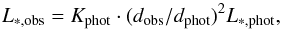 (2)where d
is the distance, L∗ ,phot is the bolometric luminosity of the
photospheric template, and L∗ ,obs is that of the input
object. With this relation, we derive L∗ for the input YSO.
(2)where d
is the distance, L∗ ,phot is the bolometric luminosity of the
photospheric template, and L∗ ,obs is that of the input
object. With this relation, we derive L∗ for the input YSO.
From Teff and L∗ we then derive R∗, whose error is derived by propagation of the uncertainties on Teff and L∗. The target M∗ and age are obtained by interpolation of evolutionary models (Siess et al. 2000; Baraffe et al. 1998; Palla & Stahler 1999; D’Antona & Mazzitelli 1994) in the position of the target on the HRD. Their typical uncertainties are determined by allowing their position on the HRD to vary according to the errors on Teff and L∗. Finally, we derive Ṁacc using the relation Ṁacc = 1.25·LaccR∗/(GM∗) (Gullbring et al. 1998), and its error is determined propagating the uncertainties on the various quantities in the relation. We report the values derived using all the evolutionary models.
Another important quantity, which can be used to asses the young age of a PMS star, is the presence and the depth of the lithium absorption line at λ ~ 670.8. Given that veiling substantially modifies the equivalent width of this line (EWLi), we need to use the reddening- and veiling-corrected spectrum of the target to derive this quantity. On this corrected spectrum, we calculate EWLi, integrating the Gaussian fit of the line, which is previously normalized to the local pseduo-continuum at the edges of the line. The statistical error derived on this quantity is given by the propagation of the uncertainty on the continuum estimate.
4. Results
In the following, we report the accretion and stellar properties of the two older PMS candidates obtained by using the procedure explained in Sect. 3.
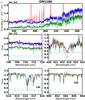 |
Fig. 2 Best fit for the object OM1186. Balmer jump, normalization region, Ca I absorption feature, and photospheric features used to check derived veiling. |
4.1. OM1186
The best fit for OM1186 is shown in Fig. 2: the red line is the observed spectrum, the green is the photospheric template, the cyan line is the slab model, and the blue is the best fit. The region around the Balmer jump is shown in the upper plot. The other panels show the normalization region around ~710 nm, the continuum normalized Ca I absorption line at ~422 nm, and the photospheric features at λ ~ 616 nm and λ ~ 844 nm. We clearly see that the agreement between the observed and best fit spectra is very good in all the region analyzed. This is obtained using a photospheric template of SpT K5, which corresponds to Teff = 4350 K with an estimated uncertainty of 350 K, AV = 0.9 ± 0.4 mag, and slab parameters leading to a value of Lacc = 0.20 ± 0.09 L⊙. We then confirm the SpT reported in the literature for this object, but we derive a different value for the extinction, which was found to be AV = 2.4 mag.
The result of the comparison of the input spectrum to the grid of synthetic spectra is shown in Fig. 3. The best agreement is found using a synthetic spectrum at the same nominal Teff of the best fit photosphere: Teff = 4350 K with log g = 4.5. In Fig. 3, both regions adopted for the log g analysis are shown, and the red line refers to the reddening- and veiling-corrected observed spectrum, while the black dotted line is the synthetic spectrum, which reproduces the observed one better. We also report the residuals in the bottom panel.
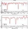 |
Fig. 3 Comparison of the reddening- and veiling-corrected spectrum of OM1186 with a synthetic spectrum with Teff = 4350 K and log g = 4.5. |
From the best fit, we derive a value of
L∗ = 1.15 ± 0.36 L⊙ for this
object. With this value and using Teff = 4350 K, we derive the
mass and age for these objects with the evolutionary models of Siess et al. (2000), Baraffe et al.
(1998), Palla & Stahler (1999),
and D’Antona & Mazzitelli (1994). The
values derived are, respectively,
M∗ = { 1.1 ± 0.4,1.4 ± 0.3, 1.1 ± 0.4,
0.6 ± 0.3} M⊙ and age =
{ ,
,
 ,
,
 ,
,
 }
Myr. Moreover, we derive Ṁacc with the parameters derived from
the fit and from the evolutionary models, and we obtain
Ṁacc = {1.3 ± 0.8, 1.1 ± 0.6, 1.4 ± 0.8,
2.4 ± 1.8} × 10-8 M⊙/yr for this object,
according to the different evolutionary tracks. From the reddening- and veiling-corrected
spectrum, we derive EWLi = 658 ± 85 mÅ.
All the parameters derived from the best fit are reported in Table 3, while those derived using the evolutionary models are in Table 4.
}
Myr. Moreover, we derive Ṁacc with the parameters derived from
the fit and from the evolutionary models, and we obtain
Ṁacc = {1.3 ± 0.8, 1.1 ± 0.6, 1.4 ± 0.8,
2.4 ± 1.8} × 10-8 M⊙/yr for this object,
according to the different evolutionary tracks. From the reddening- and veiling-corrected
spectrum, we derive EWLi = 658 ± 85 mÅ.
All the parameters derived from the best fit are reported in Table 3, while those derived using the evolutionary models are in Table 4.
Newly derived parameters from the multicomponent fit.
4.2. OM3125
For OM3125, the values reported in the literature are SpT G8-K0 and
AV = 1.47 mag. Using the same procedure,
we obtain a minimum value with a
photospheric template of SpT K7, which corresponds to
Teff = 4060 K with an uncertainty of 250 K and
AV = 1.2 ± 0.3 mag. With this best
fit model, we do not reproduce the Ca I absorption feature at
λ ~ 616.5 nm very well, because the amount of veiling in this
line is too high. Looking at the solutions with values of
similar to
the minimum value, we find that the best agreement between the observed and fitting
spectrum in this feature is with a value of
AV = 1.0 mag. Please note that the choice
of this solution instead of the one with
AV = 1.2 mag implies the same derived
parameters L∗ and Lacc well within
the errors. We show this adopted best fit in Fig. 4,
using the same color−code as in Fig. 2. The slab
model used here leads to a value of Lacc = 1.25 ± 0.60
L⊙. The effect of veiling in this object is stronger than in
OM1186, and this is clearly seen in both the Balmer jump excess and the Ca I absorption
feature at λ ~ 420 nm, which is almost completely veiled. The Ca
I absorption features has also emission on reversal of the very faint absorption feature.
Moreover, the other photospheric features are also much more veiled, as it is shown in the
bottom panels of Fig. 4. In the bottom right panel,
there are also hydrogen and helium emission lines due to accretion in correspondence with
the TiO absorption features normally present in the photosphere of objects with this SpT
(see Fig. 2 for comparison).
In Fig. 5 we show the synthetic spectrum analysis for this object, using the same color code as in Fig. 3. In this case, the best agreement is found with a synthetic spectrum with Teff = 4000 K and log g = 4.0.
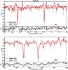 |
Fig. 5 Comparison of the reddening- and veiling-corrected spectrum of OM3125 with a synthetic spectrum with Teff = 4000 K and log g = 4.0. Same as Fig. 3. |
The luminosity derived for this object from its best fit is
L∗ = 0.81 ± 0.44 L⊙. With
this value and using Teff = 4060 K, we derive the mass and age
for these objects with the evolutionary models of Siess et
al. (2000); Baraffe et al. (1998); Palla & Stahler (1999); D’Antona & Mazzitelli (1994). The values derived are
M∗ = { 0.8 ± 0.3,1.2 ± 0.2,0.8 ± 0.2,0.5 ± 0.2 }
M⊙ and age = { ,
,
 ,
,
 ,
,
 }
Myr, respectively. According to the different evolutionary models, this object has
Ṁacc = {1.2 ± 0.9, 0.8 ± 0.5, 1.2 ± 0.7,
1.9 ± 1.2} × 10-7 M⊙/yr, and
EWLi = 735 ± 42 mÅ. These results are
also reported in Tables 3 and 4.
}
Myr, respectively. According to the different evolutionary models, this object has
Ṁacc = {1.2 ± 0.9, 0.8 ± 0.5, 1.2 ± 0.7,
1.9 ± 1.2} × 10-7 M⊙/yr, and
EWLi = 735 ± 42 mÅ. These results are
also reported in Tables 3 and 4.
Parameters derived from evolutionary models using newly derived photospheric parameters.
5. Discussion
With the results presented in the previous section, we determine new positions for our target on the HRD. This is shown in Fig. 6 with green stars representing the two YSOs analyzed in this study and the other symbols representing the rest of the ONC population, as in Fig. 1. Their revised positions are compatible with the bulk of the population of the ONC, and their revised mean ages, ~2.9 Myr for OM1186 and ~2.4 Myr for OM3125, are typical ages for objects in this region, for which the mean age has been estimated around 2.2 Myr (Reggiani et al. 2011). We also check that the final results do not depend on the value that we have chosen for the reddening law, i.e. RV = 3.1. With a value of RV = 5.0, we obtain ages, which are systematically younger than the one obtained in our analysis by a factor ~30% for OM1186 and ~50% for OM3125. With the newly determined parameters, these objects are clearly not older than the rest of the population, and their status of candidate older PMS is due to an incorrect estimate of the photospheric parameters in the literature. Figure 6 also shows that most of the objects that then appear older than 10 Myr have small or negligible Hα excess (blue circles). Among the objects with age ≳ 10 Myr, only eight objects actually show signatures of intense accretion (one red diamond visible in the plot; the other seven have Teff < 3550 K and are, therefore, outside the plot range) and at the same time of age older than 10 Myr. These objects should be observed in the future with techniques similar to the one we used here (see Sect. 5.3 for details) to understand their real nature. In the following, we analyze other derived parameters for these objects that confirm the age estimated with the HRD. Then, we address possible reasons which lead to misclassification of these targets in the literature.
5.1. Age related parameters
Lithium abundance: using the values of EWLi and the stellar parameters obtained in the previous section, we calculate the lithium abundance (log N(Li)) for the two targets by interpolation of the curves of growth provided by Pavlenko & Magazzu (1996). We derive log N(Li) = 3.324 ± 0.187 for OM1186 and logN(Li) = 3.196 ± 0.068 for OM3125. These values are compatible with the young ages of the targets, according to various evolutionary models (Siess et al. 2000; D’Antona & Mazzitelli 1994; Baraffe et al. 1998). Indeed, these models predict almost no depletion of lithium for objects with these Teff at ages less than 3 Myr, which means that the measured lithium abundance for younger objects should be compatible with the interstellar abundance of log N(Li) ~ 3.1−3.3 (Palla et al. 2007).
Surface gravity:the derived values of the surface gravity for the two targets are compatible with the theoretical values for objects with Teff ~ 4000−4350 K and an age between ~1−4.5 Myr. Indeed, both models of Siess et al. (2000) and Baraffe et al. (1998) predict a value of log g ~ 4.0 for objects with these properties. Nevertheless, the derived value of log g for OM1186 is also typical of much older objects, given that models predict log g ~ 4.5 at ages ~20 Myr with a very small increase in future evolutionary stages. However, the uncertainties on the determination of this parameter are not small, and the increase of this value during the PMS phase is usually within the errors of the measurements.
5.2. Sources of error in the previous classifications
Both targets have been misplaced on the HRD, but the reasons were different. For OM1186, we confirmed the SpT available from the literature, but we found different values of AV and Lacc with respect to Da Rio et al. (2010a). In their work, they use a color−color BVI diagram to simultaneously derive AV and Lacc with the assumption of the SpT. To model the excess emission due to accretion, they use a superposition of an optically thick emission, which reproduces the heated photosphere, and of an optically thin emission, which models the infalling accretion flow. From this model spectrum they derive the contribution of accretion to the photometric colors of the targets by synthetic photometry. Their method assumes that the positions of the objects on the BVI diagram are displaced from the theoretical isochrone due to a combination of extinction and accretion. With the assumption of the SpT, they can find the combination of parameters (AV, Lacc), which best reproduces the positions of each target on the BVI diagram. With these values, they corrected the I-band photometry for the excess due to accretion, derived using the accretion spectrum model, and for reddening effects. Finally, they derived L∗ from this corrected I-band photometry using a bolometric correction. Using this method, they found a solution for OM1186 with a large value of AV and, subsequently, accretion. Given the large amount of excess due to accretion they derive in the I-band, they underestimated L∗ and assigned an old age to this target. On the other hand, our revised photospheric parameters are compatible with those of Manara et al. (2012), who found AV = 1.16 mag, L∗ = 0.77 L⊙, and age ~ 6 Myr. In their analysis, they used the same method as Da Rio et al. (2010a), but they also had U-band photometric data at their disposal, and thus used an UBI color−color diagram. Given that the excess emission due to accretion with respect to the photosphere in the U-band is much stronger, they were able to determine the accretion properties of the targets more accurately and to find a unique correct solution.
Regarding OM3125, we derived a different SpT with respect to the one usually assumed in the literature (G8-K0; Hillenbrand 1997) with our analysis. This estimate was obtained using an optical spectrum covering the wavelength region from ~500 nm to ~900 nm, and their analysis did not consider the contribution of accretion to the observed spectrum. This was assumed not to be a strong contaminant for the photospheric features in this wavelength range. This is a reasonable assumption for objects with low accretion rates, but it was later shown not to be accurate for stronger accretors (Fischer et al. 2011), as we already pointed out for this target. In particular, strong veiling makes the spectral features shallower, which lead to an incorrect earlier classification of the target. Hillenbrand (1997) marked this SpT classification as uncertain, and they also reported the previous classification for this object from Cohen & Kuhi (1979), who classified it as being of SpT K6, a value which agrees with our finding. This previous classification is obtained using spectra at shorter wavelengths (λ ~ 420−680 nm) with respect to Hillenbrand (1997) and with no modeling of the accretion contribution. The difference in the classification is most likely because some TiO features at λλ ~ 476, 479 nm, which are typical of objects of spectral class late-K, were covered in the spectra of Cohen & Kuhi (1979). Given the large amount of veiling due to accretion that is present in the spectrum of this object, it represents a clear case where the detailed analysis carried out in our work is needed. We conclude that even optical spectra covering large regions of the spectra, like those used in Hillenbrand (1997) and in Cohen & Kuhi (1979), can lead to different and sometimes incorrect results, if the veiling contribution is not properly modeled.
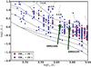 |
Fig. 6 H-R diagram of the ONC from Da Rio et al. (2012) with colored stars showing the new positions of the two targets of this study. The overplotted evolutionary tracks are from D’Antona & Mazzitelli (1994). We plot (from top to bottom) the 0.3, 1, 3, 10, 30, and 100 Myr isochrones. |
5.3. Implications of our findings
Accretion veiling, extinction, and spectral type are difficult to estimate accurately from limited datasets, especially if they are mostly based on only few photometric bands. When classifying YSOs, the difficulty increases, given that accretion and extinction may substantially modify the observed spectra. For this reason, the use of few photometric bands, where accretion, extinction, and spectral type effects can be very degenerate (e.g., B − I band range), or of spectra that cover only small wavelength regions (e.g., λ ~ 500−900 nm), can lead to different solutions, which may be incorrect.
With our work, we show that an analysis of the whole optical spectrum, which includes a detailed modeling of the various components of the observed spectrum, leads to an accurate estimate of the stellar parameters. When good quality and intermediate resolution spectra with large wavelength coverage from λ ~ 330 nm to λ ~ 1000 nm are not available, we suggest that a combination of photometric and spectroscopic data could also lead to a robust estimate of the stellar parameters of the targets independently of their SpT. In particular, the photometric data should cover the region around the Balmer jump (using both U- and B-band) and around λ ~ 700 nm (R- and I-band). With this dataset, it would be possible to derive accretion and veiling properties, extinction, and SpT by means of photometrical methods similar to those of Manara et al. (2012). This could be expanded to include different photospheric templates and different accretion spectra. At the same time, spectra in selected wavelength regions, where photospheric lines sensitive to Teff and/or log g are present, are necessary to pin-down degeneracies on the SpT. Finally, the lithium absorption line should be included as another test of the age.
Our work also implies that single objects, which deviate from the bulk of the population in nearby young clusters (age ≲3 Myr), could be affected by an incorrect estimate of the photospheric parameters, especially in cases where the determination is based on few photometric bands and the effects of veiling due to accretion and extinction are strong. On the other hand, we have no reason to believe that also a large number of objects positioned along the isochrones that represents the bulk of the population in nearby regions should be affected by similar problems. We think that the vast majority of the estimates available are correct for the following reasons. First of all, objects with low or negligible accretion should be easier to classify, given that their spectral features are not affected by veiling. Then, there are small effects in various regions due to differential extinction. In particular, we expect the amount of misclassified objects to be particularly small when dealing with objects located in regions less affected by extinction effects, such as σ-Ori. Larger numbers of objects could be misclassified in very young regions (age ≲ 1 Myr, e.g., ρ-Oph), where both accretion and extinction effects are strong. We could have here both an underestimation of L∗, as in the case of OM1186, due to an overestimation of Lacc and an overestimation of L∗ due to an underestimation of Lacc. These effects could contribute to the spread of L∗, which is observed in almost all star forming regions. Finally, accretion variability effects should not substantially affect the properties of most of the targets, given that these effects are usually small (e.g., Costigan et al. 2012).
Even though any conclusion on the nature of the older populations observed in massive clusters cannot be drawn from this work, we suggest that the method explained here or the alternative approach suggested in this section should be used to study these objects in more detail.
6. Conclusion
We have observed two candidate old (age > 10Myr) accreting PMS in the ONC with the ESO/VLT X-shooter spectrograph to confirm previous accretion rate and age estimates. Using a detailed analysis of the observed spectra based on a multicomponent fit that includes photospheric emission, the effect of reddening, and the continuum excess due to accretion, we derived revised accretion rates and stellar parameters for the two targets. We confirm that the objects are accretors as from previous studies, but the revised photospheric parameters place these objects in the same location as the bulk of the ONC young stellar population (age ~ 2−3 Myr). Therefore, they cannot be considered older PMS, but they are classical accreting YSOs. In particular, we confirmed the previously estimated SpT for OM1186, but we derived different values of AV and Lacc with respect to previous works in the literature, finding that the real position of this object on the HRD leads to a mean age estimate of ~2.9 Myr. On the other hand, we derived a different SpT for OM3125 with respect to the usually assumed value in the literature. With the other parameters, this moved this target to a position on the HRD leading to an age of ~2.4 Myr. The analysis of the lithium abundance and that of the surface gravity confirm this finding, even if the uncertainties for the latter were large.
We showed that we are able to accurately determine the stellar parameters of YSOs with our analysis, while the use of few photometric bands alone (e.g., only the B- and I-band) or of only spectra covering small wavelength regions can lead to large errors in the derived position on the HRD. We thus suggest that single objects in nearby young clusters whose position on the HRD is not compatible with the bulk of the population in their region, could be misplaced, especially if there is the suspicion of high optical veiling connected to large values of the accretion rate. The nature of these individual objects will need to be verified using a detailed analysis similar to the one reported in this study to verify the existence and to study the properties of long-lived disks around young stellar objects.
Acknowledgments
We thank the anonymous referee for providing useful comments which helped us to improve the paper. We thank the ESO Director General for awarding DDT time to this project and the ESO staff in Paranal for carrying out the observations in Service mode. We thank Andrea Banzatti for useful comments and discussion which helped to improve the fitting procedure. C.F.M. acknowledges the Ph.D. fellowship of the International Max-Planck-Research School. G.B. acknowledges the European Community’s Seventh Framework Programme under grant agreement no. 229 517.
References
- Alcalá, J. M., Natta, A., Manara, C. F., et al. 2013, A&A, submitted [Google Scholar]
- Allard, F., Homeier, D., & Freytag, B. 2011, ASP Conf. Ser., 448, 91 [NASA ADS] [Google Scholar]
- Baraffe, I., & Chabrier, G. 2010, A&A, 521, A44 [NASA ADS] [CrossRef] [EDP Sciences] [Google Scholar]
- Baraffe, I., Chabrier, G., Allard, F., & Hauschildt, P. H. 1998, A&A, 337, 403 [NASA ADS] [Google Scholar]
- Barentsen, G., Vink, J. S., Drew, J. E., et al. 2011, MNRAS, 415, 103 [NASA ADS] [CrossRef] [Google Scholar]
- Beccari, G., Spezzi, L., De Marchi, G., et al. 2010, ApJ, 720, 1108 [NASA ADS] [CrossRef] [Google Scholar]
- Cardelli, J. A., Clayton, G. C., & Mathis, J. S. 1989, ApJ, 345, 245 [NASA ADS] [CrossRef] [Google Scholar]
- Cohen, M., & Kuhi, L. V. 1979, ApJS, 41, 743 [NASA ADS] [CrossRef] [Google Scholar]
- Costigan, G., Scholz, A., Stelzer, B., et al. 2012, MNRAS, 427, 1344 [NASA ADS] [CrossRef] [Google Scholar]
- D’Antona, F., & Mazzitelli, I. 1994, ApJS, 90, 467 [NASA ADS] [CrossRef] [Google Scholar]
- Da Rio, N., Robberto, M., Soderblom, D. R., et al. 2010a, ApJ, 722, 1092 [NASA ADS] [CrossRef] [Google Scholar]
- Da Rio, N., Gouliermis, D. A., & Gennaro, M. 2010b, ApJ, 723, 166 [NASA ADS] [CrossRef] [Google Scholar]
- Da Rio, N., Robberto, M., Hillenbrand, L. A., Henning, T., & Stassun, K. G. 2012, ApJ, 748, 14 [NASA ADS] [CrossRef] [Google Scholar]
- De Marchi, G., Panagia, N., & Romaniello, M. 2010, ApJ, 715, 1 [NASA ADS] [CrossRef] [Google Scholar]
- De Marchi, G., Paresce, F., Panagia, N., et al. 2011, ApJ, 739, 27 [NASA ADS] [CrossRef] [Google Scholar]
- Fischer, W., Edwards, S., Hillenbrand, L., & Kwan, J. 2011, ApJ, 730, 73 [NASA ADS] [CrossRef] [Google Scholar]
- Gullbring, E., Hartmann, L., Briceno, C., & Calvet, N. 1998, ApJ, 492, 323 [NASA ADS] [CrossRef] [Google Scholar]
- Haisch, K. E., Jr., Lada, E. A., & Lada, C. J. 2001, ApJ, 553, L153 [NASA ADS] [CrossRef] [Google Scholar]
- Hartmann, L. 2003, ApJ, 585, 398 [NASA ADS] [CrossRef] [Google Scholar]
- Hartmann, L., Calvet, N., Gullbring, E., & D’Alessio, P. 1998, ApJ, 495, 385 [NASA ADS] [CrossRef] [Google Scholar]
- Herczeg, G. J., & Hillenbrand, L. A. 2008, ApJ, 681, 594 [NASA ADS] [CrossRef] [Google Scholar]
- Hillenbrand, L. A. 1997, AJ, 113, 1733 [NASA ADS] [CrossRef] [Google Scholar]
- Huélamo, N., Bouy, H., Pinte, C., et al. 2010, A&A, 523, A42 [NASA ADS] [CrossRef] [EDP Sciences] [Google Scholar]
- Ingleby, L., Calvet, N., Bergin, E., et al. 2011, ApJ, 743, 105 [NASA ADS] [CrossRef] [Google Scholar]
- Luhman, K. L., Stauffer, J. R., Muench, A. A., et al. 2003, ApJ, 593, 1093 [NASA ADS] [CrossRef] [Google Scholar]
- Manara, C. F., Robberto, M., Da Rio, N., et al. 2012, ApJ, 755, 154 [NASA ADS] [CrossRef] [Google Scholar]
- Manara, C. F., Testi, L., Rigliaco, E., et al. 2013, A&A, 551, A107 [NASA ADS] [CrossRef] [EDP Sciences] [Google Scholar]
- Megeath, S. T., Gutermuth, R., Muzerolle, J., et al. 2012, AJ, 144, 192 [NASA ADS] [CrossRef] [Google Scholar]
- Menten, K. M., Reid, M. J., Forbrich, J., & Brunthaler, A. 2007, A&A, 474, 515 [NASA ADS] [CrossRef] [EDP Sciences] [Google Scholar]
- Modigliani, A., Goldoni, P., Royer, F., et al. 2010, Proc. SPIE, 7737 [Google Scholar]
- Palla, F., & Stahler, S. W. 1999, ApJ, 525, 772 [NASA ADS] [CrossRef] [Google Scholar]
- Palla, F., Randich, S., Pavlenko, Y. V., Flaccomio, E., & Pallavicini, R. 2007, ApJ, 659, L41 [NASA ADS] [CrossRef] [Google Scholar]
- Pavlenko, Y. V., & Magazzu, A. 1996, A&A, 311, 961 [NASA ADS] [Google Scholar]
- Reggiani, M., Robberto, M., Da Rio, N., et al. 2011, A&A, 534, A83 [NASA ADS] [CrossRef] [EDP Sciences] [Google Scholar]
- Riaz, B., Martín, E. L., Tata, R., et al. 2012, MNRAS, 419, 1887 [NASA ADS] [CrossRef] [Google Scholar]
- Rigliaco, E., Natta, A., Testi, L., et al. 2012, A&A, 548, A56 [NASA ADS] [CrossRef] [EDP Sciences] [Google Scholar]
- Robberto, M., et al. 2013, ApJS, in press [Google Scholar]
- Siess, L., Dufour, E., & Forestini, M. 2000, A&A, 358, 593 [NASA ADS] [Google Scholar]
- Spezzi, L., de Marchi, G., Panagia, N., Sicilia-Aguilar, A., & Ercolano, B. 2012, MNRAS, 421, 78 [NASA ADS] [Google Scholar]
- Stassun, K. G., Mathieu, R. D., Mazeh, T., & Vrba, F. J. 1999, AJ, 117, 2941 [NASA ADS] [CrossRef] [Google Scholar]
- Stelzer, B., Frasca, A., Alcalá, J. M., et al. 2013, A&A, in press, DOI: 10.1051/0004-6361/201321979 [Google Scholar]
- Valenti, J. A., Basri, G., & Johns, C. M. 1993, AJ, 106, 2024 [NASA ADS] [CrossRef] [Google Scholar]
- Vernet, J., Dekker, H., D’Odorico, S., et al. 2011, A&A, 536, A105 [NASA ADS] [CrossRef] [EDP Sciences] [Google Scholar]
- White, R. J., & Basri, G. 2003, ApJ, 582, 1109 [NASA ADS] [CrossRef] [Google Scholar]
- White, R. J., & Hillenbrand, L. A. 2005, ApJ, 621, L65 [NASA ADS] [CrossRef] [Google Scholar]
- Williams, J. P., & Cieza, L. A. 2011, ARA&A, 49, 67 [NASA ADS] [CrossRef] [Google Scholar]
- Wolf, S., Malbet, F., Alexander, R., et al. 2012, A&A Rev, 20, 52 [Google Scholar]
All Tables
Spectral features used to calculate the best-fit in our multicomponent fit procedure.
Parameters derived from evolutionary models using newly derived photospheric parameters.
All Figures
|
Fig. 1 H-R diagram of the ONC from Da Rio et al. (2012) with green stars showing the positions of the two targets of this study. The overplotted evolutionary tracks are from D’Antona & Mazzitelli (1994). We plot (from top to bottom) the 0.3, 1, 3, 10, 30, and 100 Myr isochrones. |
| In the text | |
|
Fig. 2 Best fit for the object OM1186. Balmer jump, normalization region, Ca I absorption feature, and photospheric features used to check derived veiling. |
| In the text | |
|
Fig. 3 Comparison of the reddening- and veiling-corrected spectrum of OM1186 with a synthetic spectrum with Teff = 4350 K and log g = 4.5. |
| In the text | |
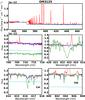 |
Fig. 4 Best fit for the object OM3125. Same as Fig. 2. |
| In the text | |
|
Fig. 5 Comparison of the reddening- and veiling-corrected spectrum of OM3125 with a synthetic spectrum with Teff = 4000 K and log g = 4.0. Same as Fig. 3. |
| In the text | |
|
Fig. 6 H-R diagram of the ONC from Da Rio et al. (2012) with colored stars showing the new positions of the two targets of this study. The overplotted evolutionary tracks are from D’Antona & Mazzitelli (1994). We plot (from top to bottom) the 0.3, 1, 3, 10, 30, and 100 Myr isochrones. |
| In the text | |
Current usage metrics show cumulative count of Article Views (full-text article views including HTML views, PDF and ePub downloads, according to the available data) and Abstracts Views on Vision4Press platform.
Data correspond to usage on the plateform after 2015. The current usage metrics is available 48-96 hours after online publication and is updated daily on week days.
Initial download of the metrics may take a while.