| Issue |
A&A
Volume 558, October 2013
|
|
|---|---|---|
| Article Number | A30 | |
| Number of page(s) | 10 | |
| Section | The Sun | |
| DOI | https://doi.org/10.1051/0004-6361/201321719 | |
| Published online | 30 September 2013 | |
Temporal relation between quiet-Sun transverse fields and the strong flows detected by IMaX/SUNRISE
1 Instituto de Astrofísica de Canarias, 38200 La Laguna, Tenerife, Spain
e-mail: cqn@iac.es
2 Departamento de Astrofísica, Univ. de La Laguna, 38205 La Laguna, Tenerife, Spain
3 Kiepenheuer-Institut für Sonnenphysik, Schöneckstr. 6, 79104 Freiburg, Germany
4 Max-Planck-Institut für Sonnensystemforschung, Max-Planck-Str. 2, 37191 Katlenburg-Lindau, Germany
5 School of Space Research, Kyung Hee University, Yongin, 446-701 Gyeonggi, Republic of Korea
Received: 17 April 2013
Accepted: 8 August 2013
Context. Localized strongly Doppler-shifted Stokes V signals were detected by IMaX/SUNRISE. These signals are related to newly emerged magnetic loops that are observed as linear polarization features.
Aims. We aim to set constraints on the physical nature and causes of these highly Doppler-shifted signals. In particular, the temporal relation between the appearance of transverse fields and the strong Doppler shifts is analyzed in some detail.
Methods. We calculated the time difference between the appearance of the strong flows and the linear polarization. We also obtained the distances from the center of various features to the nearest neutral lines and whether they overlap or not. These distances were compared with those obtained from randomly distributed points on observed magnetograms. Various cases of strong flows are described in some detail.
Results. The linear polarization signals precede the appearance of the strong flows by on average 84 ± 11 s. The strongly Doppler-shifted signals are closer (0.″19) to magnetic neutral lines than randomly distributed points (0.″5). Eighty percent of the strongly Doppler-shifted signals are close to a neutral line that is located between the emerging field and pre-existing fields. That the remaining 20% do not show a close-by pre-existing field could be explained by a lack of sensitivity or an unfavorable geometry of the pre-existing field, for instance, a canopy-like structure.
Conclusions. Transverse fields occurred before the observation of the strong Doppler shifts. The process is most naturally explained as the emergence of a granular-scale loop that first gives rise to the linear polarization signals, interacts with pre-existing fields (generating new neutral line configurations), and produces the observed strong flows. This explanation is indicative of frequent small-scale reconnection events in the quiet Sun.
Key words: Sun: photosphere / Sun: surface magnetism / Sun: granulation
© ESO, 2013
1. Introduction
The analysis of the quiet-Sun magnetism has been enormously advanced in the past years (see, e.g., de Wijn et al. 2009; Martinez Pillet 2013, for recent reviews). A crucial aspect in this achievement has been the successful performance of instruments onboard the Hinode (see Kosugi et al. 2007; Tsuneta et al. 2008) and SUNRISE missions (see Barthol et al. 2011; Solanki et al. 2010). They have both provided quantitative data with spatial resolutions similar to or better than those available in the past and very significantly improved the temporal consistency, going beyond the typical granular evolutionary timescales. Supplemented with a polarimetric sensitivity of, typically, one part in 103, these observational conditions have allowed the characterization of the horizontal component of quiet-Sun fields. It has been found that they typically appear at locations with intermediate continuum intensities (Lites et al. 2008; Danilovic et al. 2010a), near the edges of granules (as originally found by the Advanced Stokes Polarimeter, ASP Lites et al. 1996), and have a clear transient nature (Ishikawa & Tsuneta 2009b; Danilovic et al. 2010a). The temporal evolution of these high-quality polarimetric data can often be described as loops emerging at the surface (Martínez González et al. 2007; Centeno et al. 2007), protruding into various heights in the atmosphere (Martínez González & Bellot Rubio 2009), and with a characteristic non-uniform spatial distribution of the emerging loops that displays “dead calm” areas (Martínez González et al. 2012; Lites et al. 2008, who previously reported on these non-uniform distributions).
High-speed Doppler-shifted signals have been found in a number of cases in the quiet-Sun fields, mostly seen in the Stokes V parameter (see a variety of examples in Shimizu et al. 2008). The convective-collapse process first proposed on theoretical grounds by Parker (1978), Webb & Roberts (1978), and Spruit (1979) has been tentatively identified in the works of Bellot Rubio et al. (2001) and Nagata et al. (2008) as the amplification of the magnetic field induced by a strong downflow of cold material (Danilovic et al. 2010b). The line-of-sight (LOS) component of these downflows reaches speeds of 6 km s-1. It has also been proposed that these downflows hit dense layers and rebound into upflows with supersonic speeds as well (Grossmann-Doerth et al. 1998), which would explain the extremely blueshifted signals observed by Socas-Navarro & Manso Sainz (2005).
Perhaps the most unexpected discovery made with the IMaX/SUNRISE instrument (see Martínez Pillet et al. 2011a) is the detection of subarcsecond patches of circular polarization at the continuum reference wavelength point of this instrument (Borrero et al. 2010). In its normal observing mode, this magnetograph maps the Fe i line in 5250.2 Å in four wavelength points within the line and one in the continuum region mid-range between this line and the neighboring Fe i 5250.6 Å line. The exact continuum point is at 227 mÅ from the IMaX line center. As stated by Borrero et al. (2010), the only way to generate circular polarization signals at this continuum wavelength is by Doppler-shifting either one of the Fe i line signals there. The fact that most of the observed continuum polarization patches occurred on top of upflowing granules led these authors to suggest that the patches were produced by upflows that shift the Fe i 5250.6 Å line to the continuum point. The estimated LOS velocities needed to generate these shifts were in the range [5, 12] km s-1 (Borrero et al. 2012). Because both opposite polarity patches and transverse fields were seen close to the location of the continuum polarization patches, some form of reconnection between newly emerged loops and surrounding fields was proposed as the most plausible scenario for their occurrence. More recently, Borrero et al. (2013) have used data from the same instrument, but with better spectral coverage, to perform inversions that result in increased heating in the upper layers and in opposite polarities along the LOS. This result further consolidates the hypothesis of a reconnection-driven process. The presence of these highly Doppler-shifted signals at what, otherwise, are continuum wavelengths has been confirmed in Hinode/SP data, as shown by Martínez Pillet et al. (2011b). The superior spectral sampling of the Hinode/SP instrument allowed a clear separation of blueshifted and redshifted events (which these authors termed quiet-Sun jets), which was not possible with the single-continuum point of IMaX/SUNRISE. These authors confirmed the transverse field regions in the surroundings of the jets and found a tendency for quiet-Sun jets to occur in blue- and redshifted pairs.
The chronological relation between the transverse field patches and the jets remains unclear from these studies (we continue the naming convention proposed by Martínez Pillet et al. 2011b): is there a preference for the transverse signals or for the jets to occur first? If reconnection is driven by the emergence of new magnetic bipoles into the solar atmosphere, it is expected that the transverse signals precede the detection of the jets. Taking advantage of the large FOV and good temporal cadence of the IMaX/SUNRISE data, we study in this work the temporal sequence of the detection of the transverse fields and the jets. Other aspects of this phenomenon, such as the distance of the jets to the nearest neutral line and some case examples of transverse fields that preceded the jets, are discussed at some length.
2. Observations and data analysis
We used the same two data sets as Borrero et al. (2010). They were recorded on June 9, 2009 and have a duration of 22.6 and 31.9 min, respectively. The field of view (FOV) is 47′′ × 47′′. The data were recorded in the IMaX V5-6 mode (Martínez Pillet et al. 2011a), which sampled five wavelength positions relative to λ0 = 5250.217 Å: −80, −40,40,80 mÅ, and a fifth wavelength placed at the continuum: λc = λ0 + 227 mÅ. The instrument obtained the four Stokes parameters (I,Q,U,V)† with a time cadence of 33 s and a pixel size of 0 055. Six accumulations were summed in this mode to achieve a signal-to-noise ratio of 103. The instrument made periodic calibrations of the optical aberrations by using a phase diversity glass plate that generates a known out-of-focus configuration in one of the two cameras used to measure the orthogonal polarization states. These calibrations can be used to perform an image restoration of the data and bring it closer to the diffraction limit. This restoration process also increases the noise, so that for some detection purposes it may not be as well suited as the non-restored data. Specifically, the noise increases by a factor 3 in the restored frames. Indeed, to identify the nearly horizontal fields, we used the non-restored linear polarization signal averaged over the four wavelength positions in the spectral line, as in Danilovic et al. (2010a). The above-mentioned increase of noise in the restored Q and U frames allows only the stronger linear polarization patches to be detected in the restored data. The strong flows were detected also using the non-restored circular polarization signal at λc. However, when using the normal magnetograms to identify the nearest neutral-line both, the non-restored and restored data were included in the analysis.
The events (jets and transverse fields) were detected manually. We established their intensity and size thresholds to identify them. First, we include in the analysis linear polarization signals above 0.26% of the continuum level and circular polarization signals at the continuum wavelength, Vc, above 0.4% (also normalized to the continuum intensity). Second, the selected events had to reach a minimum area of five pixels in Vc and the corresponding linear polarization patch sometime during their evolution. We used the identification of a jet event in Vc as reference. Then we searched for a nearby, concurrent linear polarization patch. This patch could occur before or after the first detection of the highly Doppler-shifted signal.
The total number of jets found is 96, 72 of which (75%) show a clear relation with a linear polarization patch, while the rest of the events does not show a connection with any enhanced linear polarization region. These results closely agree with the work of Borrero et al. (2010), who used the restored data to characterize properties such as the physical dimensions of the events for which the nearly diffraction-limited data are better suited.
3. Results
The aim of this section is to study the temporal relation between the jets and the associated linear polarization patches. We also quantify the typical distances between these features and their nearest neutral line. Because in the quiet-Sun observed by IMaX/SUNRISE neutral lines are frequently encountered, a comparison of these distances with those found for randomly defined locations is mandatory. These studies can help us to stablish a possible scenario for the occurrence of the quiet-Sun jets and complement the works of Borrero et al. (2010, 2012) and Martínez Pillet et al. (2011b).
3.1. Temporal relation between Vc jets and the associated linear polarization regions
We first quantified the time difference between the initial instant at which we saw the signal at Vc and the first moment at which we detected the associated transverse field patch. Some of the 72 cases of quiet-Sun jets associated to linear polarization signals were not included in the analysis because the associated transverse field region was already present at the beginning of the time series. For these cases only a lower limit could be estimated and we decided not to include them. A precise time interval could be defined for only 60 cases.
The histograms of the time differences in Fig. 1 reveal that the associated linear polarization patches precede the strong Vc jets in most of the cases, by 84 ± 11 s on average. It seems clear therefore that the Doppler-shifted signals are a consequence of the small-scale flux emergence processes, as shown by the linear polarization patches. Only 13% of the cases show a negative value, indicating that the jets are seen before the corresponding transverse field region. It is important, however, to bear in mind that the two types of signals are highly affected by visibility effects. On the one hand, the Vc signals are enhanced when a large component of the underlying flow is aligned with the LOS. On the other hand, the linear polarization signals are always very sensitive to the exact field line configuration and strength. As a consequence, jets associated with small-scale flux emergence could be more frequent than determined here (or in Borrero et al. 2010) and, often, we might not detect the linear polarization signals simply because of low field strengths, small features, or both, resulting in low flux entities that are hidden below the noise level. These visibility problems might help explain the relatively large standard deviation observed in Fig. 1 (91 s). We also calculated the median of the data sets because the shape of the distribution is not always clearly symmetric. We provide the opportunity to examine the results from the mean and the median values of the distributions, although these two values are very close throughout the analysis.
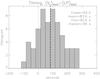 |
Fig. 1 Histogram of the time difference between the beginning of the Vc jet signal and the appearance of the linear polarization signal. Positive values mean that the linear polarization precedes the appearance of the highly Doppler shifted signal. The thick dashed line represents the averaged time difference. |
3.2. Distance to the nearest neutral line
The fact that the jets have a clear preference to occur after the emergence of the small-scale loop indicates that the evolution of the loop once it is at the surface and its interaction with possible surrounding fields might trigger the process. The existence of these granular scale magnetic loops in the photosphere has already been clearly established by various observations (De Pontieu 2002; Centeno et al. 2007; Martínez González & Bellot Rubio 2009; Ishikawa & Tsuneta 2009a; Ishikawa et al. 2010). In the previous studies of Borrero et al. (2010, 2012) and Martínez Pillet et al. (2011b) all evidence pointed to the possibility that some form of reconnection of the newly emerged loops with pre-existing fields triggers the high-speed flows. To additionally consolidate this possibility, we study in this section the distance of the Vc events to the nearest neutral line in the FOV. The location of a jet event is defined by an intensity-weighted position estimated by 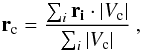 (1)where ri is the distance from each pixel of the event that displays a Vc signal to a reference system’s origin defined in a small FOV of 100 × 100 pixels, or
  , which was used to individually analyze the events. From this location we then perform an automated search for the closest neutral line and measured the smallest distance between them. Neutral lines are identified in edge-enhanced magnetograms that can be easily thresholded to display the pixels where neutral lines are found. For this purpose we used the IDL procedure sobel.pro, which is based on the Sobel edge-enhancement operator. It is a local non-linear operator that detects gradients between pixels in an image to give information about the edges of the structures displayed in that image. An example of the selected pixels corresponding to our definition of the neutral line configuration is presented in Fig. 2. Pixels inside the blue contours are considered as neutral lines. The distance from the locations of Vc events (as defined in Eq. (1)) to the nearest neutral line is given by the closest pixel inside the blue line contours encountered in the neighborhood.
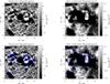 |
Fig. 2 Example of neutral line identification in one IMaX/SUNRISE magnetogram. The left column corresponds to restored and the right column to non-restored magnetograms (but they represent the same observations). The top row displays the original magnetograms, the bottom row overlays the neutral lines (blue contours) identified by the edge-enhancement procedure explained in the text. Note the increased frequency of neutral lines occurrences in the restored data. |
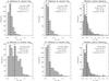 |
Fig. 3 Histograms of distances between various features and neutral lines. The first column shows the distances between the centers of the non-restored Vc jets to the neutral lines defined on the restored (top) and on the non-restored magnetogram (bottom). The second column shows the same quantity for the linear polarization patches. The third column presents the distances of randomly distributed points to their nearest neutral lines. |
The restored magnetograms offer a much higher resolution for the detection of neutral lines than the non-restored ones, and the former often show neutral lines that are not seen in the latter. But because we define the locations of Vc jets and linear polarization patches only in the non-restored magnetograms, we used the neutral lines found in the non-restored magnetograms in addition to those from the restored magnetograms. The center of the transverse patches was defined in a similar way as for the Vc signals defined in Eq. (1), but now weighting with the amount of the observed linear polarization. We also estimated distances of randomly distributed points over the FOV to their nearest neutral lines to compare with the obtained distances of the jets and of the linear polarization patches to the nearest neutral line. Comparing the distances measured for linear polarization patches and Vc jets is interesting because for the first ones (which represent magnetic loops that always contain a neutral line) we expect to deduce smaller distances than for the Vc events. Similarly, randomly distributed points are expected to provide distances to the nearest neutral line that gauge how likely it is to be close to one such line in the IMaX magnetograms by chance. If the jet events are related to magnetic reconnection processes, we expect them to be closer to the neutral lines than the randomly distributed points. Note that this step is not needed to evaluate the possible effect of erroneous detections of Vc jets and/or neutral lines, but as a way of establishing a statistically meaningful reference of a spatial correlation between these features.
Jet events are often detected in several IMaX snapshots, for each of them an estimate of the distance to the nearest neutral line is obtained. They evolve in time in a way that shows proper motions (see Borrero et al. 2010) that reflect the evolution of the underlying granulation, it is not clear which instant is more representative of the proximity to a neutral line. Thus, all of the above estimates were included in the analysis. For these reasons, the 60 associated cases produce a total of 365 distance values for the Vc jets and 465 values for the associated linear polarization patches. Accordingly, we chose to study 500 randomly placed points to provide a similar statistical comparison.
Figure 3 provides the histograms of the various distances obtained from the non-restored Vc jets, the non-restored linear polarization patches, and the randomly placed points to the neutral lines detected on the restored and non-restored magnetograms (top and bottom rows, respectively). The histograms for the randomly distributed points show that the typical distance to a neutral line in an IMaX/SUNRISE magnetogram is only 05 (in both the restored and non-restored magnetograms). However, the typical distance of a Vc jet is much smaller, around 019 for the reconstructed data. In agreement with the predictions above, the average distance of the center of the linear polarization patches to the nearest neutral line is smaller, about 016. This number nicely coincides with the spatial resolution of the data (Martínez Pillet et al. 2011a). Interestingly, the same ordering in the magnitudes of the distances is obtained for the non-restored data, with the random points located farthest from the neutral lines, followed by the jets and finally the linear polarization signals as the closest ones. This consolidates the same trend as was found for the restored magnetograms and demonstrates that the Vc jets detected by IMaX/SUNRISE are significantly closer to quiet-Sun neutral lines than randomly selected points. Thus, these results additionally support the hypothesis that these jets originate from reconnection events in the photosphere that are associated with, and usually follow, the emergence of small-scale quiet-Sun loops.
3.3. Relative distances between Vc jets and transverse field patches
With the above estimates, we studied the distance distribution of the quiet-Sun jets and the associated linear polarization patches. Note that in Borrero et al. (2010) this distance was not estimated and the association between horizontal patches and Vc events was considered real as long as it was smaller than 2′′. Of all locations measured in the different snapshots, a total of 229 snapshots offered a clear correspondence between jets and transverse fields, allowing an estimate of their separation. The total number of distances is lower than the number used in Fig. 3. The reason is that almost every associated event presents a linear polarization patch that occurs before the Vc jet, and during these periods of time a proper distance cannot be measured. Then, the jet appears near the linear polarization patch, allowing one to measure the distance between them. Finally, some cases show that the linear polarization patch vanishes before the Vc jet, providing a situation where the distances between them cannot be measured again.
Figure 4 provides the histogram of these distances with a mean value of 057. These distances are measured in the non-restored data because linear polarization patches are not easily detected in the restored data (due to the increased noise in them). Thus, to compare this with the results of the previous section, one should use the values from the bottom row in Fig. 3. In particular, the mean distance of Vc jets to neutral lines in the non-restored data is 041. This value is lower than the mean distance between the center of the Vc jets and the center of the linear polarization patch. This indicates that the jets have, on average, a neutral line closer to them than the one corresponding to the associated linear polarization patch. This tendency has been confirmed by visual inspection in 80% of the cases analyzed. The remaining 20% are different in the sense that the closest neutral line to the Vc signal is the one of the associated linear polarization patch. Below we discuss different examples of these two types.
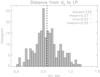 |
Fig. 4 Distances between Vc jets and the associated linear polarization patches as measured in the non-restored data. |
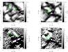 |
Fig. 5 Two examples of the most common configuration found (80 % of the associated events) where the linear polarization patch (green) is closer to a neutral line different from the one that is nearest to the Vc jet (purple). The top row displays a continuum map in which the linear polarization signals always appear at the edges of granules. The bottom row shows the restored magnetograms. This configuration exemplifies the conclusions from Figs. 3 and 4. |
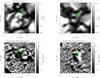 |
Fig. 6 Two examples of the less common configuration (only 20% of the associated cases) where the linear polarization patch (green) and the Vc jet (purple) are related to the same neutral line configuration. The images displayed correspond to the same quantities as given in Fig. 5. |
In Fig. 5, two events of the first type are shown. In them, a newly emerged loop, identified by the transverse fields (green contours) and the two footpoints of opposite polarity in the underlying (restored) magnetogram, generate a Vc jet (purple contour). The jet is closer to a neutral line different from the one associated to the loop’s footpoints. This other neutral line is created by the interaction of one of the footpoints with a pre-existing field region of opposite polarity. In the first example in this figure, two loops are seen. The jet is closer to the smaller one in the middle of the image. The top footpoint of this loop is of positive polarity and the bottom one of negative polarity.
This last footpoint encounters a small positive polarity field region and the Vc jet is seen on this side of the loop, on top of the negative polarity footpoint. It seems natural to associate the jet with this closer neutral line and not with the one overlying the loop itself. The second example corresponds to a larger transverse patch where the negative polarity of the loop encounters a tiny round positive polarity element of 02 diameter that seems to be responsible for the Vc jet in this case. Note the many other lines in both pictures without any linear polarization (which consequently are not newly emerged quiet-Sun loops) or Vc signals.
Figure 6 shows two examples of newly emerged loops that display Vc jets whose position is closer to the neutral line created by the loop itself (representing 20% of the cases). The first example shows a large transverse field patch that intersects most of the Vc jet area. The loop is asymmetric and the negative polarity occupies a larger area than the positive one. Even if other neutral lines are seen nearby (to the right of the linear polarization patch), the jet is closer to the neutral line that is seen inside the green contour. A more obvious case is displayed in the second example of this figure, where an isolated loop is shown with both the green and purple contours intersecting the neutral line that is created by the opposite polarity footpoints of the loop. No other observed neutral line can be argued to be responsible for the jet signal in this case.
It is also of interest how systematically the transverse field regions are located at the borders of granules (Lites et al. 1996, 2008; Danilovic et al. 2010a), as shown by the continuum frames in Figs. 5 and 6.
3.4. Description of a complex case
While the majority of the jets observed in these two time series correspond to an association of one linear polarization patch and a single Vc feature, a few cases have been observed that show multiple high-speed flows triggered by linear polarization patches. We describe here the most complex of these associations observed with IMaX/SUNRISE, including its evolution, and how the jets respond to the varying granulation pattern.
A clarification is in order beforehand. The circular polarization signals in the continuum, Vc, are a signed quantity. So far we have not discussed the signs of the observed jets. The example explained here displays Vc of both signs. However, in the case of the IMaX observation, it is hard to make a sensible use of the observed signs of the Vc in these jets. Because the continuum point used in this instrument is midway between the Fe i 5250.2 Å and the Fe i 5250.6 Å lines, a blueshift or redshift can give rise to oppositely signed signals at λc. Besides, if one compares jets with the same flow directions but opposite magnetic orientations of the LOS component, the signs of the corresponding Vc signals are reversed as well. Thus, if we observe two Vc jets next to each other with different signs, it is impossible to distinguish between opposite flow directions and/or opposite field line orientations. Data with better spectral coverage are needed to achieve this. One could assume that the sign of the magnetic or velocity field in the jet atmosphere is the same as that inferred from the four points inside the spectral line. But this assumption is not fully justified before the nature of quiet-Sun jets is better understood.
Figure 7 covers almost 20 min of a 6 × 6 arcsec2 area from the first time series. In this area, the most complex jet event observed by IMaX/SUNRISE was detected. The background of each snapshot corresponds to the continuum intensity and allows examining the evolution of the granular pattern during the event. As before, green contours designate the linear polarization signals, but now the Vc contours indicate the sign of the events in blue (positive Vc) and red (negative Vc). The event develops mostly negative Vc jets but also creates positive Vc signals for a short period of time. As explained before, this can only be taken as an indication that either oppositely directed strong flows or opposite polarity fields participate in the event. Time is given in seconds from the beginning of the full observed data set. The corresponding reconstructed magnetograms are shown in Fig. 8.
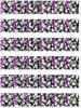 |
Fig. 7 Evolution of the most complex Vc jet observed with IMaX/SUNRISE. The images correspond to the continuum intensity. Linear polarization is represented by green contours over the granular pattern. Blue and red contours correspond to positive and negative Vc signals. Time (given in each frame) runs from left to right, starting at the top (as seen by turning the page on its side). Units given with the maps are in arcsec. |
A large patch of linear polarization is first seen at t = 132 s located at the edge of a granule and progressively increases in size. Since the first snapshot was taken a few scattered pixels near that patch show negative signal at λc (see the red pixels close to the patch). At t = 330 s, the event reaches a temporary maximum with a clear jet-transverse field association. After this time, the transverse field patch slightly fades, but never disappears completely. Interestingly, at t = 462 s, a positive polarity jet starts to develop and attains a maximum at t = 627 s. Positive/negative associations of jets with clear upflow/downflow components were observed in Martínez Pillet et al. (2011b) using Hinode/SP data. While this positive Vc component disappears two snapshots later, the negative (red) component of the jet and the transverse field patch again increase. The strongest development of the event occurs in the interval t = [858,1122] s. In this interval, around t = 990 s, the negative Vc jet has broken into two adjacent patches that move in opposite directions as the horizontal field patch increases in size. The two periods with increasing linear polarization signals coincide with a similar increase of the associated granule. Periods of decreasing linear polarization signal (t = [429,627] s) coincide with granular break-up. This reinforces the relation of these events with flux emergence episodes connected with granular upflows. From a magnetic point of view (see Fig. 8), this case is different from the previous ones studied in the sense that, now, a multipolar structure seems to be emerging. At t = 495 s or at t = 693 s, two patches with opposite polarity footpoints are seen. The system only resolves into a more or less bipolar structure at the very end, in the second phase of increasing linear polarization signals (t = 1188 s). In the present case, no pre-existing fields seem to be playing a major role (although they cannot be completely ruled out), and one would favor jets triggered by interactions of the intrinsically tangled (multipolar) topology of the magnetic structure.
Figure 7 also shows the onset of an isolated blue jet at the edge of a granule near the bottom of the t = 363 s snapshot. This strong flow is generated with no clear connection to any linear polarization patch and constitutes an isolated jet. It stays visible until t = 495 s (see Fig. 7). Interestingly, a loop is seen at a later time t = 528 s (see Fig. 8). We therefore assume that here a transverse field emerged at the time at which the jet was detected, but it did not produce strong enough Stokes Q and/or U signals to be detected by IMaX/SUNRISE.
4. Discussion
The evidence presented in this paper supports the original idea presented in Borrero et al. (2010, 2012) and Martínez Pillet et al. (2011b) for the origin of the quiet-Sun jets detected by IMaX/SUNRISE. Granular upflows are connected with surfacing small-scale flux loops. The first evidence of these loops was obtained from a linear polarization patch that preceded any signature of a strong flow most of the time. These flux loops often have a bipolar configuration but, sometimes, more complex configurations are encountered. The neutral lines created by the loop’s footpoints are naturally observed below them at the spatial resolution of the observations. Most jets are systematically located at larger distances from the transverse field regions than from nearby neutral lines formed between the emerging fields and pre-existing ones. In a small number of cases no transverse fields are seen before the jet, which might be explained by a lack of sensitivity to the linear polarization signals. In approximately 20% of the cases we were unable to identify a nearby neutral line with a pre-existing field. We speculate that in these events we missed a weak pre-existing field due to insufficient sensitivity to the circular polarization signals. Thus, the sequence of flux loop emergence and interaction with pre-existing fields might be valid to explain more or less all quiet-Sun jets.
The physical mechanism that is most naturally invoked to explain high-speed flows, the Vc jets, is magnetic reconnection. The recent work of Borrero et al. (2013) has shown from full radiative-transfer Stokes inversions that magnetic fields with different inclinations along the line-of-sight and temperature increases are needed to fit the profiles. This strongly favors reconnection as the underlying mechanism.
The most complex case observed, which showed a multipolar configuration, might be better explained as interactions among the different polarity footpoints of the structure itself that also lead to reconnection processes. There is a clear tendency for both the transverse field patches and the Vc jets to appear near the edges of granules (the former result dates back to Lites et al. 1996). Their evolution follows the granular expansion. All in all, it would seem that the loops interact and reconnect with pre-existing fields after being pushed by the granules to the edges, where they encounter the fields in the nearby intergranular regions. There reconnection events are finally triggered. Vc jets of opposite sings (in the observed circular polarization at λc) naturally arise from the coexistence of different field orientations and oppositely directed flows as a result of the reconnection.
We note that because the emerging fields seem to be passively advected by the granulation, the field strengths should be around or below equipartition with the convective flows. The results presented here and in the previously cited works indicate that these weak fields are nonetheless capable of generating the observed high-speed flows when reconnecting. Note, however, that the pre-existing field also involved in the reconnection may well be strong (see Lagg et al. 2010). While further studies are needed to consolidate magnetic reconnection as the physical mechanism responsible for them, other possibilities should not be excluded. The intrinsically larger number of redshifted events found by Martínez Pillet et al. (2011b) indicates that strong downflows may be initiated by some other physical mechanism, such as convective collapse (Parker 1978; Grossmann-Doerth et al. 1998; Nagata et al. 2008; Shimizu et al. 2008; Fischer et al. 2009; Danilovic et al. 2010b). The association between upflows and downflows encountered by Martínez Pillet et al. (2011b) could be reminiscent of some form of siphon-flow process (Rueedi et al. 1992; Montesinos & Thomas 1993). Finally, it is known that granular evolution itself leads to supersonic (horizontal) flows (Cattaneo et al. 1989; Solanki et al. 1996; Bellot Rubio 2009) that could play a role in generating the observed Vc events.
5. Conclusions
We quantitatively analyzed the relation between quiet-Sun jets described by Borrero et al. (2010) and the transverse field patches observed with IMaX/SUNRISE. In particular, the timing relation between them and the distances of these features to nearby neutral lines observed in magnetograms were quantified. The results can be summarized as follows:
In 77% of the cases for which a clear association between transverse fields and Vc jets could be established, we found that the transverse fields occur before the jets, on average by about 84 s, and always by less than 300 s, a typical granulation timescale.
Vc jets have a mean distance to nearby neutral lines of 019. This is significantly shorter than the distance of randomly distributed points in IMaX/SUNRISE magnetograms from neutral lines (05). This reinforces the association of these processes with reconnection events. However, 019 is larger than the spatial resolution of the data, so that the jets are associated with neutral lines, but not necessarily overlap them.
The transverse field patches have a typical distance of 016 to a neutral line, which is close to the spatial resolution of the data. Because they occur more often over granular regions, these patches are more easily interpreted in terms of magnetic loop emergence (Danilovic et al. 2010a).
The distance between Vc jets and the transverse patches is typically 057 (as measured in the non-reconstructed data), larger than the typical distance between jets and the nearest neutral lines.
Visual inspection showed that 80% of the Vc jets are closer to neutral lines that are generated between one of the loop’s footpoints and a pre-existing field of opposite polarity than to the neutral line between the loop footpoints. The remaining 20% of the Vc jets can only be associated to the neutral line of the recently emerged loop. We cannot rule out that we missed pre-existing fields in these cases because of the limited sensitivity of the observations.
Complex cases with multipolar configurations and repeated Vc jet events can also occur.
Both the transverse field regions and the Vc jets evolve following the underlying granular pattern, in particular, they occur near the edges of the granules most of the time.
All these results support the suggestion that quiet-Sun jets are a result of the interaction of a newly emerged granular loop with already existing fields, which triggers magnetic reconnection. One observable signature of this reconnection are the Vc jets. It is clear, however, that to fully characterize these processes, analyses of data with better spectral coverage that include several magnetically sensitive lines are needed. In addition, a study of the signatures of these jets at different limb distances would be very useful. Work is in progress to perform such studies using Hinode and SUNRISE data, to obtain a better
understanding of the physical process. In addition, an MHD simulation of emerging magnetic flux and its interaction with a pre-existing field would provide valuable physical insight.
Acknowledgments
We thank Eric Priest for interesting discussions on the possible nature of these quiet-Sun jets. This work has been partially funded by the Spanish MINECO through Project No. AYA200AYA2011-29833-C06 and by the WCU grant No. R31-10016 funded by the Korean Ministry of Education, Science and Technology.
References
- Barthol, P., Gandorfer, A., Solanki, S. K., et al. 2011, Sol. Phys., 268, 1 [NASA ADS] [CrossRef] [Google Scholar]
- Bellot Rubio, L. R. 2009, ApJ, 700, 284 [NASA ADS] [CrossRef] [Google Scholar]
- Bellot Rubio, L. R., Rodríguez Hidalgo, I., Collados, M., Khomenko, E., & Ruiz Cobo, B. 2001, ApJ, 560, 1010 [NASA ADS] [CrossRef] [Google Scholar]
- Borrero, J. M., Martínez Pillet, V., Schlichenmaier, R., et al. 2010, ApJ, 723, L144 [NASA ADS] [CrossRef] [Google Scholar]
- Borrero, J. M., Pillet, V. M., Schlichenmaier, R., et al. 2012, in 4th Hinode Science Meeting: Unsolved Problems and Recent Insights, eds. L. Bellot Rubio, F. Reale, & M. Carlsson, ASP Conf. Ser., 455, 155 [Google Scholar]
- Borrero, J. M., Martínez Pillet, V., Schmidt, W., et al. 2013, ApJ, 768, 69 [NASA ADS] [CrossRef] [Google Scholar]
- Cattaneo, F., Hurlburt, N. E., & Toomre, J. 1989, in Solar and Stellar Granulation, eds. R. J. Rutten, & G. Severino, NATO ASIC Proc., 263, 415 [Google Scholar]
- Centeno, R., Socas-Navarro, H., Lites, B., et al. 2007, ApJ, 666, L137 [NASA ADS] [CrossRef] [Google Scholar]
- Danilovic, S., Beeck, B., Pietarila, A., et al. 2010a, ApJ, 723, L149 [NASA ADS] [CrossRef] [Google Scholar]
- Danilovic, S., Schüssler, M., & Solanki, S. K. 2010b, A&A, 509, A76 [NASA ADS] [CrossRef] [EDP Sciences] [Google Scholar]
- De Pontieu, B. 2002, ApJ, 569, 474 [NASA ADS] [CrossRef] [Google Scholar]
- de Wijn, A. G., Stenflo, J. O., Solanki, S. K., & Tsuneta, S. 2009, Space Sci. Rev., 144, 275 [NASA ADS] [CrossRef] [Google Scholar]
- Fischer, C. E., de Wijn, A. G., Centeno, R., Lites, B. W., & Keller, C. U. 2009, in The Second Hinode Science Meeting: Beyond Discovery-Toward Understanding, eds. B. Lites, M. Cheung, T. Magara, J. Mariska, & K. Reeves, ASP Conf. Ser., 415, 127 [Google Scholar]
- Grossmann-Doerth, U., Schuessler, M., & Steiner, O. 1998, A&A, 337, 928 [NASA ADS] [Google Scholar]
- Ishikawa, R., & Tsuneta, S. 2009a, A&A, 495, 607 [NASA ADS] [CrossRef] [EDP Sciences] [Google Scholar]
- Ishikawa, R., & Tsuneta, S. 2009b, in The Second Hinode Science Meeting: Beyond Discovery-Toward Understanding, eds. B. Lites, M. Cheung, T. Magara, J. Mariska, & K. Reeves, ASP Conf. Ser., 415, 132 [Google Scholar]
- Ishikawa, R., Tsuneta, S., & Jurčák, J. 2010, ApJ, 713, 1310 [NASA ADS] [CrossRef] [Google Scholar]
- Kosugi, T., Matsuzaki, K., Sakao, T., et al. 2007, Sol. Phys., 243, 3 [NASA ADS] [CrossRef] [Google Scholar]
- Lagg, A., Solanki, S. K., Riethmüller, T. L., et al. 2010, ApJ, 723, L164 [NASA ADS] [CrossRef] [Google Scholar]
- Lites, B. W., Leka, K. D., Skumanich, A., Martinez Pillet, V., & Shimizu, T. 1996, ApJ, 460, 1019 [NASA ADS] [CrossRef] [Google Scholar]
- Lites, B. W., Kubo, M., Socas-Navarro, H., et al. 2008, ApJ, 672, 1237 [NASA ADS] [CrossRef] [Google Scholar]
- Martínez González, M. J., & Bellot Rubio, L. R. 2009, ApJ, 700, 1391 [CrossRef] [Google Scholar]
- Martínez González, M. J., Collados, M., Ruiz Cobo, B., & Solanki, S. K. 2007, A&A, 469, L39 [NASA ADS] [CrossRef] [EDP Sciences] [Google Scholar]
- Martínez González, M. J., Manso Sainz, R., Asensio Ramos, A., & Hijano, E. 2012, ApJ, 755, 175 [NASA ADS] [CrossRef] [Google Scholar]
- Martinez Pillet, V. 2013, Space Sci. Rev., in press [arXiv:1301.6933] [Google Scholar]
- Martínez Pillet, V., Del Toro Iniesta, J. C., Álvarez-Herrero, A., et al. 2011a, Sol. Phys., 268, 57 [NASA ADS] [CrossRef] [Google Scholar]
- Martínez Pillet, V., Del Toro Iniesta, J. C., & Quintero Noda, C. 2011b, A&A, 530, A111 [NASA ADS] [CrossRef] [EDP Sciences] [Google Scholar]
- Montesinos, B., & Thomas, J. H. 1993, ApJ, 402, 314 [NASA ADS] [CrossRef] [Google Scholar]
- Nagata, S., Tsuneta, S., Suematsu, Y., et al. 2008, ApJ, 677, L145 [NASA ADS] [CrossRef] [Google Scholar]
- Parker, E. N. 1978, ApJ, 221, 368 [NASA ADS] [CrossRef] [Google Scholar]
- Rueedi, I., Solanki, S. K., & Rabin, D. 1992, A&A, 261, L21 [NASA ADS] [Google Scholar]
- Shimizu, T., Lites, B. W., Katsukawa, Y., et al. 2008, ApJ, 680, 1467 [NASA ADS] [CrossRef] [Google Scholar]
- Socas-Navarro, H., & Manso Sainz, R. 2005, ApJ, 620, L71 [NASA ADS] [CrossRef] [Google Scholar]
- Solanki, S. K., Rueedi, I., Bianda, M., & Steffen, M. 1996, A&A, 308, 623 [NASA ADS] [Google Scholar]
- Solanki, S. K., Barthol, P., Danilovic, S., et al. 2010, ApJ, 723, L127 [NASA ADS] [CrossRef] [Google Scholar]
- Spruit, H. C. 1979, Sol. Phys., 61, 363 [NASA ADS] [CrossRef] [Google Scholar]
- Tsuneta, S., Ichimoto, K., Katsukawa, Y., et al. 2008, Sol. Phys., 249, 167 [NASA ADS] [CrossRef] [Google Scholar]
- Webb, A. R., & Roberts, B. 1978, Sol. Phys., 59, 249 [NASA ADS] [CrossRef] [Google Scholar]
All Figures
|
Fig. 1 Histogram of the time difference between the beginning of the Vc jet signal and the appearance of the linear polarization signal. Positive values mean that the linear polarization precedes the appearance of the highly Doppler shifted signal. The thick dashed line represents the averaged time difference. |
| In the text | |
|
Fig. 2 Example of neutral line identification in one IMaX/SUNRISE magnetogram. The left column corresponds to restored and the right column to non-restored magnetograms (but they represent the same observations). The top row displays the original magnetograms, the bottom row overlays the neutral lines (blue contours) identified by the edge-enhancement procedure explained in the text. Note the increased frequency of neutral lines occurrences in the restored data. |
| In the text | |
|
Fig. 3 Histograms of distances between various features and neutral lines. The first column shows the distances between the centers of the non-restored Vc jets to the neutral lines defined on the restored (top) and on the non-restored magnetogram (bottom). The second column shows the same quantity for the linear polarization patches. The third column presents the distances of randomly distributed points to their nearest neutral lines. |
| In the text | |
|
Fig. 4 Distances between Vc jets and the associated linear polarization patches as measured in the non-restored data. |
| In the text | |
|
Fig. 5 Two examples of the most common configuration found (80 % of the associated events) where the linear polarization patch (green) is closer to a neutral line different from the one that is nearest to the Vc jet (purple). The top row displays a continuum map in which the linear polarization signals always appear at the edges of granules. The bottom row shows the restored magnetograms. This configuration exemplifies the conclusions from Figs. 3 and 4. |
| In the text | |
|
Fig. 6 Two examples of the less common configuration (only 20% of the associated cases) where the linear polarization patch (green) and the Vc jet (purple) are related to the same neutral line configuration. The images displayed correspond to the same quantities as given in Fig. 5. |
| In the text | |
|
Fig. 7 Evolution of the most complex Vc jet observed with IMaX/SUNRISE. The images correspond to the continuum intensity. Linear polarization is represented by green contours over the granular pattern. Blue and red contours correspond to positive and negative Vc signals. Time (given in each frame) runs from left to right, starting at the top (as seen by turning the page on its side). Units given with the maps are in arcsec. |
| In the text | |
 |
Fig. 8 Same as Fig. 7, but with the reconstructed magnetograms as background images. |
| In the text | |
Current usage metrics show cumulative count of Article Views (full-text article views including HTML views, PDF and ePub downloads, according to the available data) and Abstracts Views on Vision4Press platform.
Data correspond to usage on the plateform after 2015. The current usage metrics is available 48-96 hours after online publication and is updated daily on week days.
Initial download of the metrics may take a while.