| Issue |
A&A
Volume 558, October 2013
|
|
|---|---|---|
| Article Number | A42 | |
| Number of page(s) | 15 | |
| Section | Extragalactic astronomy | |
| DOI | https://doi.org/10.1051/0004-6361/201321652 | |
| Published online | 01 October 2013 | |
The planetary nebula population in the halo of M 87⋆
1
Max-Planck-Institut für Extraterrestrische Physik,
Giessenbachstrasse,
85741
Garching, Germany
e-mail: This email address is being protected from spambots. You need JavaScript enabled to view it.
; This email address is being protected from spambots. You need JavaScript enabled to view it.
2
European Southern Observatory, Karl-Schwarzschild-Strasse 2, 85748
Garching,
Germany
e-mail: This email address is being protected from spambots. You need JavaScript enabled to view it.
3
Department of Advanced Sciences, Faculty of Science and
Engineering, Hosei University, 184-8584
Tokyo,
Japan
e-mail: This email address is being protected from spambots. You need JavaScript enabled to view it.
4
RSAA, Mt. Stromlo Observatory, 2611
Camberra,
Australia
e-mail: This email address is being protected from spambots. You need JavaScript enabled to view it.
Received:
5
April
2013
Accepted:
15
August
2013
Abstract
Aims. We investigate the diffuse light in the outer regions of the nearby elliptical galaxy M 87 in the Virgo cluster, in the transition region between galaxy halo and intracluster light (ICL).
Methods. The diffuse light is traced using planetary nebulas (PNs). The surveyed areas are imaged with a narrow-band filter centred on the redshifted [OIII]λ5007 Å emission line at the Virgo cluster distance (the on-band image) and with a broad-band V-filter (the off-band image). All PNs are identified through the on-off band technique using automatic selection criteria based on the distribution of the detected sources in the colour–magnitude diagram and the properties of their point-spread function.
Results. We present the results of an imaging survey for PNs within a total effective area of 0.43 deg2, covering the stellar halo of M 87 up to a radial distance of 150 kpc. We extract a catalogue of 688 objects down to m5007 = 28.4, with an estimated residual contamination from foreground stars and background Lyα galaxies, which amounts to ~35% of the sample. This is one of the largest extragalactic PN samples in number of candidates, magnitude depth, and radial extent, which allows us to carry out an unprecedented photometric study of the PN population in the outer regions of M 87. We find that the logarithmic density profile of the PN distribution is shallower than the surface brightness profile at large radii. This behaviour is consistent with a model where the luminosity specific PN numbers for the M 87 halo and ICL are different. Because of the depth of this survey we are also able to study the shape of the PN luminosity function (PNLF) in the outer regions of M 87. We find a slope for the PNLF that is steeper at fainter magnitudes than the standard analytical PNLF formula and adopt a generalised model that treats the slope as a free parameter.
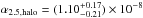
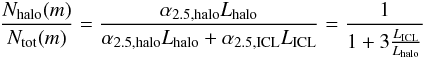
Conclusions. The logarithmic PN number density profile is consistent with the superposition of two components associated with the halo of M 87 and with the ICL, which have different α parameters. We derive α2.5,halo = (1.10-0.21+0.17) × 10-8 NPN L⊙,bol-1 and α2.5,ICL = (3.29-0.72+0.60) × 10-8 NPN L⊙,bol-1 for the halo and the intracluster stellar components, respectively. The fit of the generalised formula to the empirical PNLF for the M 87 halo returns a value for the slope of 1.17 and a preliminary distance modulus to the M 87 halo of 30.74. Comparing the PNLF of M 87 and the M 31 bulge, both normalised by the sampled luminosity, the M 87 PNLF contains fewer bright PNs and has a steeper slope towards fainter magnitudes.
Key words: galaxies: groups: individual: M 87 / planetary nebulae: general / galaxies: elliptical and lenticular, cD / galaxies: clusters: general / galaxies: halos
Tables 4 and 5 are available in electronic form at http://www.aanda.org
© ESO, 2013
1. Introduction
Stars in the mass range between 1 and 8 M⊙ go through the planetary nebula (PN) phase before ending their lives as white dwarfs. The optical image of a PN is dominated by the luminous ionized envelope that is powered by the stellar core at its centre. The envelope emits in several strong lines from the UV to the NIR, and Dopita et al. (1992) showed that up to 15% of the luminosity of the central star is re-emitted in the forbidden [OIII] line at λ5007 Å.
PNs have been used as kinematic tracers of the stellar orbital distribution in the outer regions of galaxies, where the continuum from the stellar surface brightness is too low with respect to the night sky, both in nearby galaxies (Hui et al. 1993; Peng et al. 2004; Merrett et al. 2006; Coccato et al. 2009; Cortesi et al. 2013) and out to 50–100 Mpc (Ventimiglia et al. 2011; Gerhard et al. 2005). The outer regions of galaxies are particularly interesting because dynamical times are longer there, so they may preserve information of the mass assembly processes.
The observed properties of the PN population in external galaxies also correlate with the age and metallicity of the parent stellar population. These properties are the luminosity-specific PN number, α-parameter for short, that quantifies the stellar luminosity associated with a detected PN, and the shape of the PN luminosity function (PNLF). We discuss these in turn.
Observationally the values of α correlate with the integrated (B − V) colour of the parent stellar population, with the spread in observed values for the reddest galaxies increasing significantly with respect to the constant value observed in bluer ((B − V) < 0.8) objects (Hui et al. 1993; Buzzoni et al. 2006). For the reddest galaxies, the value of α correlates with the (FUV − V) colour, with the lowest number of PNs observed in old and metal-rich systems (Buzzoni et al. 2006).
To describe the shape of the PNLF for extragalactic PN populations, the analytical formula proposed by Ciardullo et al. (1989) has generally been used, but see also models by Méndez et al. (1993, 2008). At the brightest magnitudes the PNLF shows a cutoff that is observed to be invariant between different Hubble types and has been used as secondary distance indicator (Ciardullo et al. 2004). From about one magnitude fainter than the PNLF cutoff, the analytical formula predicts an exponential increase, in agreement with the slow PN fading rate described by Henize & Westerlund (1963). Observationally, the PNLF slope correlates with the star formation history of the parent stellar population, with steeper slopes observed in older stellar populations and flat or slightly decreasing slopes in younger populations (Ciardullo et al. 2004; Ciardullo 2010).
The Virgo cluster, its elliptical galaxies, and intracluster light (ICL) were the targets of several PN surveys (Ciardullo et al. 1998; Feldmeier et al. 1998, 2004; Arnaboldi et al. 2002, 2003, 2004; Castro-Rodríguez et al. 2003, 2009; Aguerri et al. 2005), aimed at measuring distances and the ICL spatial distribution. In this paper we report the results of a deep survey carried out with the Suprime-Cam at the Subaru telescope to study the PN population in the halo around M 87, one of the two brightest galaxies in the Virgo cluster.
NGC 4486 (M 87) is a giant elliptical galaxy situated at the centre of the subcluster A in the Virgo cluster (Binggeli et al. 1987), the nearest large scale structure in the local universe. According to current models of structure formation, M 87 acquired its mass over a long period of time through galaxy mergers and mass accretion. The stars in M 87 are old (Liu et al. 2005), and its stellar halo contains about 70% of the galaxy’s light down to μV ~ 27.0 mag arcsec-2 (Kormendy et al. 2009). Thus M 87 is an ideal target for a survey aimed at detecting PNs in an extended galaxy halo, when investigating the halo kinematics and stellar population.
The paper is organized as follows: in Sect. 2 we describe the Suprime-Cam PN survey and the data reduction procedure. In Sect. 3 we describe the PN catalogue extraction and validation. The relation between the spatial distribution of the PN candidates and the M 87 surface brightness profile is investigated in Sect. 4. We present the PNLF measured in the M 87 halo in Sect. 5 and discuss the comparison with the PNLF for the M 31 bulge. Finally, we summarize our conclusions in Sect. 6. In the rest of the paper we adopt a distance modulus of 30.8 for M 87, which means that the physical scale is 73 pc arcsec-1.
2. The Suprime-Cam M 87 PN survey
2.1. Imaging and observations
In March 2010 we observed two fields with the Suprime-Cam 10 k × 8 k mosaic camera, at
the prime focus of the 8.2 m Subaru telescope (Miyazaki
et al. 2002). The CCDs have a readout noise of 10 e− and an average
gain of 3.1 e− ADU-1. Each field of view covers an area of 34′× 27′,
with a pixel size of 0 2; the two pointings cover the halo of M 87
out to a radial distance of 150 kpc. Figure 1 shows a
deep V-band image of the Virgo cluster core region and the two fields
studied in this work overlaid. We label these fields as the M 87 SUB1 and M 87 SUB2
fields, respectively.
2; the two pointings cover the halo of M 87
out to a radial distance of 150 kpc. Figure 1 shows a
deep V-band image of the Virgo cluster core region and the two fields
studied in this work overlaid. We label these fields as the M 87 SUB1 and M 87 SUB2
fields, respectively.
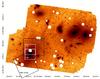 |
Fig. 1 The core of the Virgo cluster (Mihos et al. 2005) with the positions of the fields studied in this work (black rectangles) and in previous surveys by Ciardullo et al. (1998) and Feldmeier et al. (2003) (dotted white squares). The region is dominated by the halos of 3 bright galaxies, M 84, M 86 and M 87, with M 87 covered by the Suprime-Cam fields. North is up, East is to the left. |
Both fields were observed through an [OIII] narrow-band filter (on-band filter), centred on λc = 5029 Å with a band width Δλ = 74 Å and a broad-band V-filter (off-band filter). The total exposure time for the on-band images was ~3.7 h and ~4.3 h, while for the off-band images it was 1 h and 1.4 h, for the M 87 SUB1 and M 87 SUB2 fields, respectively. Deep V-band images are needed for the colour selection of the PN candidates (see Sect. 3).
Our strategy for data acquisition was set up to achieve the best image quality. Narrow-band and broad-band images were taken close to each other during the observing nights to secure similar conditions in terms of scattered light and atmospheric seeing, while calibration images, such as dark sky1, were taken in between the science images to have a similar signal-to-noise ratio and image quality.
Summary of the field positions, filter characteristics, exposure times, and seeing for the narrow-band (on-band) and broad-band (off-band) images.
The nights were photometric with an overall seeing on the images less than 1″. Airmasses were 1.01 and 1.06 for the reference M 87 SUB1 [OIII] and V-band exposures, and 1.13 and 1.03 for the reference M 87 SUB2 [OIII] and V-band exposures2. We did not perform any measurements for the extinction coefficients. We adopted the mean value of X = 0.12 mag/airmass, as listed for the [OIII] and V filters at the Mauna Kea summit web site3, and in agreement with Buton et al. (2013).
The on-band filter bandpass was designed such that its central wavelength coincides with the redshifted λ5007 Å emission at the Virgo cluster. The Johnson V-band filter can be used as the off-band filter despite the fact that it contains the [OIII] line in its large bandpass (~1000 Å). The depth of the Suprime-Cam survey was chosen to detect all PNs brighter than m∗ + 2.5, where m∗ is the [OIII]5007 Å apparent magnitude of the bright cutoff of the PNLF for a distance modulus 30.8. Table 1 gives a summary of the field positions, filter characteristics and exposure times for the on-band and off-band exposures for the analysed area around M 87.
2.2. Data reduction, astrometry and flux calibration
The removal of instrumental signature, geometric distortion correction, background (sky
plus galaxy) subtraction, a first astrometric solution and the final image combination
were done using standard data reduction packages developed for Suprime-Cam data (sdfred
software v2.04). Cosmic rays identification and
rejection were carried out with L.A. Cosmic (Laplacian Cosmic Ray Identification)
algorithm (van Dokkum 2001). Because of the
spectroscopic follow-up our aim was to derive accurate positions of the PN candidates. To
do this we improved the astrometry of the images to get a relative positional accuracy
with less than  in the residuals. The astrometric solution
was computed using image astrometry tasks in the IRAF5 package imcoords, performing a geometrical transformation by
2nd order polynomial fitting. All images analysed in this paper are on the astrometric
reference frame of the 2MASS catalogue6.
in the residuals. The astrometric solution
was computed using image astrometry tasks in the IRAF5 package imcoords, performing a geometrical transformation by
2nd order polynomial fitting. All images analysed in this paper are on the astrometric
reference frame of the 2MASS catalogue6.
We flux calibrated the broad-band and narrow-band frames to the AB system by observing standard stars through the same filters used for the survey. We used spectrophotometric standard star Hilt600 and Landolt stars for the [OIII]-band and V-band flux calibrations respectively, giving zero points for the [OIII] and V-band frames equal to Z[OIII] = 24.29 ± 0.04 and Z[V] = 27.40 ± 0.17, normalised to a 1 second exposure7.
However, the integrated flux from the [OIII] line of a PN is usually expressed by the
magnitude m5007 using the relation introduced by Jacoby (1989):
 (1)where F5007 is in
units of ergs cm-2 s-1. From this we determined the absolute flux
calibration for the nebular flux in the [OIII] emission line, following Jacoby et al. (1987). This flux calibration takes the
filter transmission efficiency at the wavelength of the emission line into account, due to
the fact that the fast optics of wide-field instruments, such as the Suprime-Cam at the
Subaru telescope can affect the transmission properties of the interference filter,
especially for narrow-band imaging. This effect was quantified making use of the filter
transmission curve described in Arnaboldi et al.
(2003), representing the expected transmission of the [OIII] interference filter
in the f/1.86 beam of the Suprime-Cam at the Subaru telescope.
(1)where F5007 is in
units of ergs cm-2 s-1. From this we determined the absolute flux
calibration for the nebular flux in the [OIII] emission line, following Jacoby et al. (1987). This flux calibration takes the
filter transmission efficiency at the wavelength of the emission line into account, due to
the fact that the fast optics of wide-field instruments, such as the Suprime-Cam at the
Subaru telescope can affect the transmission properties of the interference filter,
especially for narrow-band imaging. This effect was quantified making use of the filter
transmission curve described in Arnaboldi et al.
(2003), representing the expected transmission of the [OIII] interference filter
in the f/1.86 beam of the Suprime-Cam at the Subaru telescope.
The relation between the m5007 and
mAB magnitudes for the narrow-band filter
is given by: 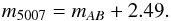 (2)A detailed description of the relation
between AB and m5007[OIII] magnitudes is
given in Arnaboldi et al. (2002).
(2)A detailed description of the relation
between AB and m5007[OIII] magnitudes is
given in Arnaboldi et al. (2002).
In this paper we will use the notation of mn and mb to refer to the narrow-band and broad band magnitudes of the objects in the AB system. We will use m5007 to refer to the [OIII] magnitudes introduced by Jacoby (1989).
Table 2 gives the constant value for AB-to-m5007 magnitude conversion, and limiting magnitudes in the on-band and off-band frames analysed in this paper.
On-band and off-band limiting magnitudes.
The final products for the M 87 SUB1 and M 87 SUB2 pointings consist of the stacked images in the [OIII] and V band, astrometrically and photometrically calibrated. As consequence of the observing strategy the seeing measured as the average FWHM of stellar sources is similar in both pairs of images, and less than FWHMseeing < 1″ (see Table 1). A fit of the PSF with the IRAF task psf (in the digiphot/daophot package) shows that a Moffat analytical function with a β parameter β = 2.5 (see IRAF/digiphot manual for more details) is the best profile to model the stellar light distribution of point sources in our images. Moreover, the PSF fit was computed in three different regions of the on-band and off-band images for both the M 87 SUB1 and M 87 SUB2 fields, covering the images from the centre to the edges: for all regions examined, the PSF fit gave the same best fit solution, showing that the PSF does not vary across the images.
3. Selection of PN candidates and catalogue extraction
As a result of their bright [OIII] (λ5007) and faint continuum emission, extragalactic PNs can be identified as objects detected in images taken through the on-band [OIII] filter, but not detected in images taken through the off-band continuum filter. In our work, all PN candidates are extracted through the on-off band technique (Jacoby et al. 1990) using selection criteria based on the distribution of the detected sources in colour magnitude diagrams (Theuns & Warren 1997). We used an automatic extraction procedure developed and validated in Arnaboldi et al. (2002, 2003) for the identification of emission line objects in our images. We give a brief summary of the selection procedure in the next section.
3.1. Extraction of point-like emission-line objects
We employed the object detection algorithm SExtractor (Bertin & Arnouts 1996), that detects and measures flux from point-like and extended objects. Sources were detected in the on-band image requiring that 20 adjacent pixels or more have flux values 1 × σ rms above the background. Magnitudes were then measured in a fixed aperture of radius R = 6 pixels (1.2″, ~3 times the seeing radius) for sources in the on-band image, and then through the aperture photometry in the V-band image at the (x,y) positions of the detected [OIII] sources with SExtractor in dual-image mode. Candidates for which SExtractor could not detect a mb magnitude at the position of the [OIII] emitter were assigned a mb = 28.7, i.e. the flux from an [OIII] emission of mn = mlim,n seen through a V-band filter (Theuns & Warren 1997). All objects were plotted in a colour magnitude diagram (CMD), mn − mb vs. mn, and classified according to their positions in this diagram. Based on their strong [OIII] line emission, the most likely PN candidates are point-like objects with colour excess corresponding to an observed EW greater than 110 Å, after convolution with photometric errors as function of the magnitude. The limit of completeness is defined as the magnitude at which the recovery fraction of an input simulated point-like population with a given luminosity function8, drops below a threshold set to 50%. We find mlim,5007 = 28.39; this is the limiting magnitude of our sample.
The colour selection of PN candidates requires off-band images deep enough so that the colour can be measured reliably at fainter magnitudes. As for the [OIII] images, we define the V-band limiting magnitude as the faintest magnitude at which half of the input simulated sample is retrieved from the image; we then derive mlim,b = 26.4 and mlim,b = 26.6 for the M 87 SUB1 and M 87 SUB2 fields respectively.
3.1.1. Colour selection
PN candidates are defined as objects with [OIII] magnitudes brighter than the [OIII] limiting magnitude and with a colour excess, mn ≤ mlim,n and mn − mb < −0.99, the latter representing the colour excess corresponding to EWobs = 110 Å. The relation between the observed EW and the colour in magnitudes is given by Teplitz et al. (2000): EWobs ≃ Δλnb(100.4Δm − 1), where Δλnb is the width of the narrow band filter and Δm = mb − mn is the colour. A value of EWobs = 110 Å limits contamination from [OII]λ3726.9 emitters at redshift z ~ 0.34 (see Sect. 3.2).
Photometric errors may be responsible for continuum emission sources falling below the adopted colour excess, hence contaminating the emission object distribution. This effect is limited by defining regions in which 99% and 99.9% of a simulated continuum population would fall in this CMD. Below the 99.9% line, the probability to detect stars is reduced to the 0.1% level.
Theoretically a PN is a point-like source with no detected continuum, i.e. with no broadband magnitude measured by Sextractor. Nevertheless we expect a continuum contribution in an aperture at the position of a [OIII] source in the halo of M 87 because of crowding effects or residuals from the subtraction of the continuum light from the M 87 halo. This is confirmed by the distribution of colours measured for a simulated PN population in the outer regions of M 87, which we discuss in Sect. 3.1.4.
3.1.2. Point-like versus extended sources
At a distance of ~15 Mpc, PNs are unresolved points of green light. We need to distinguish them from spatially extended background galaxies and, possibily, HII regions. Point-like objects in our catalogue are candidates that satisfy the following criteria:
-
1.
we compare the SExtractor mn and mcore magnitudes, where mcore represents the measured magnitude in a fixed aperture of radius R = 2 pixels (0.4″). For point-like objects mn − mcore has a constant value as function of magnitude, while it varies for extended sources. We analyzed this difference for simulated point-like objects and determined the range of mn − mcore as function of mn where 96% of the simulated population fall. This range is narrow for bright magnitudes but it becomes wider towards fainter magnitudes due to the photometric errors.
-
2.
We derive the distribution for the SExtractor half-light radius Rh, i.e. the radius within which half of the object’s total flux is contained. For point-like objects this value should be constant but due to photometric errors it is confined to a range 1 ≤ Rh ≤ 4 pixels that we determine as the range in which 95% of the simulated population lies.
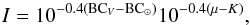
These criteria for the selection of point-like sources are shown in Fig. 2. For the simulated population, 91% of the input sources are recovered as point-like objects. Therefore, applying these criteria to the observed objects excludes 9% of the PNs from the sample along with the extended objects.
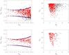 |
Fig. 2 Point-source test, showing mn − mcore vs. mn (left) and mn vs. Rh (right) for observed sources satisfying our colour restrictions in the M 87 SUB1 field (top) and for modeled point-like emission objects (bottom). The dark lines in the left panels delimit the region within which 96% of the modeled point-like emission objects fall. Observed sources in the top panels are considered as point-like objects if they lie in this region and have a half light radius in the range 1 ≤ Rh ≤ 4 pixels. This range of Rh was chosen such that 95% of the modeled population was included. Red dots represent objects that satisfy both criteria and are thus selected as point-like objects. These criteria are also applied to sources in M 87 SUB2 field. |
3.1.3. Masking of bad/noisy regions
The last step of our automatic selection is the masking of the areas where the detection and photometric measurements of sources are dominated by non-Poisson noise. These areas include diffraction and bleed spikes from the brightest stars, bad pixel regions and higher background noise regions, the latter mostly at the edges of the images because the dithering strategies lead to different exposure depth near the edges (we will discuss this further in Sect. 3.1.5). After these regions are excluded, the total effective area of our survey is ~0.43 deg2.
The selection described above leads to a catalogue, hereafter called automatic sample, containing 792 objects classified as PN candidates. These sources are point-like objects with colour excess, corresponding to an observed equivalent width EWobs > 110 Å and are located in regions of the colour–magnitude diagram where the contamination by foreground stars is below 0.1%.
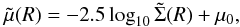
Figure 3 shows the colour selection for the M 87 SUB1 and M 87 SUB2 fields, with the PN candidates represented by asterisks.
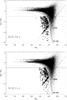 |
Fig. 3 CMD for all sources in the M 87 SUB1 (top panel) and M 87 SUB2 (bottom panel) fields. The horizontal lines indicate the colour excess of emission line objects with an EWobs = 110 Å. The curved lines delimit the regions above which 99% and 99.9% of the simulated continuum objects fall in this diagram, given the photometric errors. The set of points on the inclined line represents those objects with no broadband magnitude measured by SExtractor (see Sect. 3.1 for more details). Asterisks represent objects classified as PNs according to the selection criteria discussed in Sect. 3.1. |
3.1.4. Missing PNs in the photometric sample
The selection procedure based on flux thresholds is sensitive to photometric errors. At fainter magnitudes, PN candidates with intrinsic EWobs > 110 Å, or mn ≤ mlim,n, can have smaller measured EWobs, or fainter mn, because of photometric errors and are, therefore, excluded from our selection. We quantified this effect by simulating an [OIII] emission line population, with an exponential LF in the magnitude range 23 ≤ m ≤ 27.5, randomly distributed on the on-band scientific image. No continuum emission was assigned to the objects. We then carried out the photometry as for the real sources: their CMD is shown in Fig. 4. We see that many simulated PNs have a measured continuum magnitude due to crowding effects or residuals from the galaxy background. This CMD shows also that for simulated sources brighter than the limiting magnitude, the percentage of PNs that we would miss due to photometric errors is 28.3% and 29.8% in the M 87 SUB1 and M 87 SUB2 fields respectively. This implies that our automatic procedure, within the magnitude range 23 ≤ mn ≤ mlim,n, recovers 0.71 of the total sample. In Table 5 we show the dependence of this colour completeness on magnitude.
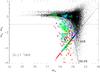 |
Fig. 4 CMD for a simulated PN population in the M 87 SUB1 field with intrinsic magnitudes 23 ≤ mn ≤ mlim,n (crosses). Because of photometric errors, our selection criteria would exclude 28.3% of the input sample (blue crosses). The remaining 71.7% would be selected as PNs (red crosses). Dots surrounded by green squares and cyan triangles are emission objects in common between our sample and the PN samples selected by Ciardullo et al. (1998) and Feldmeier et al. (2003), respectively. Solid lines as in Fig. 3. |
3.1.5. Catalogue validation: visual inspection and joint candidates in both fields
Finally, the photometric catalogue obtained from the automatic selection described in the previous sections was visually inspected, in particular for regions near bright stars or with a higher noise level. This visual inspection led to a catalogue of 688 candidates, the removed spurious detections being ~11% of the automatic extracted sources.
In the final catalogue 18 candidates appear in both fields and their magnitudes are measured independently in the two pointings. Differences between the independent measurements are consistent with the errors.
3.2. Possible sources of contaminants in the PN sample
Following Aguerri et al. (2005), we examined the main contaminants and estimate their contributions to the final catalogue.
Contamination by faint continuum objects – At mlim,n, the faint continuum objects can mimic an [OIII] emission line population, because they are scattered into the region where PN candidates are selected. We constrained this contribution by computing the 99.9% lines for the distribution of continuum objects. From the total number of the observed foreground stars, we determine the number of objects (0.1%) that would be scattered in the region of colour selected PNs. The resulting contribution from faint stars equals 9% and 11% of the total extracted sample for the M 87 SUB1 and M 87 SUB2 fields, respectively.
Contamination by background galaxies: Lyman α galaxies and [OII] emitters – The strong [OIII] λ5007 PN emission with no associated detected continuum allows us to identify PNs as objects with negative colour (Theuns & Warren 1997). This colour selection will also identify Lyα galaxies at redshift z ~ 3.1 as well as [OII] λ3727.26 emitters at redshift z ~ 0.34, whose emission lines fall within the bandpass of our narrow band filter.
The contamination by Lyα is quantified by using the number density of
z = 3.1 Lyα galaxies from Gronwall et al. (2007) where their limiting magnitude of
mlim,n(G07)(5007) = 28.31 for statistical completeness makes
their survey as deep as ours. We consider their Lyα LF given by a
Schechter function of the form:  (3)with their best-fit values of
log10L∗ = 42.66 erg s-1 and
α = −1.36, corrected for the effects of photometric errors and their
filter’s non-square transmission curve. At redshift z = 3.1, the surveyed
area of 0.43 deg2, observed through the Suprime-Cam narrow-band filter, samples
~3.1 × 10⁵ Mpc3 (Hogg
1999). However, as pointed out by Gronwall et al.
(2007), when working with narrow band data taken through a nonsquare filter
bandpass, the effective survey volume is ~25% smaller than that inferred from the
interference filter’s FWHM. We thus compute the number of expected Lyα
emitters by using a survey volume of ~2.3 × 10⁵ Mpc3. The
Lyα population at z ~ 3.1 shows clustering over a
correlation length of r0 = 3.6 Mpc (Gawiser et al. 2007), corresponding to an angular size in the Virgo
cluster of
(3)with their best-fit values of
log10L∗ = 42.66 erg s-1 and
α = −1.36, corrected for the effects of photometric errors and their
filter’s non-square transmission curve. At redshift z = 3.1, the surveyed
area of 0.43 deg2, observed through the Suprime-Cam narrow-band filter, samples
~3.1 × 10⁵ Mpc3 (Hogg
1999). However, as pointed out by Gronwall et al.
(2007), when working with narrow band data taken through a nonsquare filter
bandpass, the effective survey volume is ~25% smaller than that inferred from the
interference filter’s FWHM. We thus compute the number of expected Lyα
emitters by using a survey volume of ~2.3 × 10⁵ Mpc3. The
Lyα population at z ~ 3.1 shows clustering over a
correlation length of r0 = 3.6 Mpc (Gawiser et al. 2007), corresponding to an angular size in the Virgo
cluster of  . Hence we need to allow for the
large-scale cosmic variance in the average Lyα density, which in our case
is ~20% (Somerville et al. 2004; Gawiser et al. 2007). From our effective sampled
volume, we predict, then, that the number of expected Lyα contaminants is
25% ± 5% of our total catalogue.
. Hence we need to allow for the
large-scale cosmic variance in the average Lyα density, which in our case
is ~20% (Somerville et al. 2004; Gawiser et al. 2007). From our effective sampled
volume, we predict, then, that the number of expected Lyα contaminants is
25% ± 5% of our total catalogue.
The contribution from [OII] emitters is considerably reduced by selecting candidates with observed equivalent width, EWobs > 110 Å, corresponding to a colour threshold mn − mb < −0.99 (Teplitz et al. 2000). This is because no [OII] emitters with EWobs > 95 Å have been found (Colless et al. 1990; Hammer et al. 1997; Hogg et al. 1998). Note that in the Gronwall et al. (2007) sample of Lyα galaxies at z = 3.1, the fraction of [OII] contaminants is considered to be negligible because of their EW selection (Δm(G07) ~ −1). This means that if there is a fraction of [OII] emitters with EWobs > 110 Å in our sample, then their contribution is accounted for by using the Lyα LF from Gronwall et al. (2007).
3.3. Comparison with previous PN samples in M 87
Our survey area overlaps with those studied by Jacoby et al. (1990), Ciardullo et al. (1998, hereafter C98) and Feldmeier et al. (2003, hereafter F03); the locations of the C98 and F03 fields are over-plotted on Fig. 1.
We have a limited number of objects in common between Jacoby et al. (1990) and our catalogue (~14% of their catalogue), because of the high residual background in our images from the bright central regions of M 87. These fractions are larger for the C98 and F03 catalogues, and we discuss them in turn.
C98 carried out an [OIII] λ5007 survey for PNs, covering a 16′ × 16′ field around M 87. They identified 329 PNs in the M 87 halo, 187 of these in a statistically complete sample down to m5007 = 27.15. Of the 329 sources selected by C98, 201 fall within our surveyed area9. Of these sources, 91% are matched with [OIII] detected objects in our survey, but only ~60% satisfy our selection criteria for PN candidates, see the CMD for the C98 candidates (green squares) in Fig. 4.
F03 carried out a survey of intracluster PNs (ICPNs) over several fields in the Virgo cluster region; the one overlapping with the current Subaru survey is a 16′ × 16′ area north of M 87, labeled “FCJ” field in F03 and Aguerri et al. (2005). 100% of the candidates in this field match with [OIII] sources in the M 87 SUB1 field, but only 42% satisfy the selection criteria for PN candidates in our survey, see the CMD for the F03 candidates (cyan triangles) in Fig. 4.
On the basis of the common PN candidates with the largest signal-to-noise ratios, we can compare the photometric calibration for the m5007 magnitudes and any variations with magnitude in the different samples. We find a constant offset that does not vary with magnitude between the C98, F03 samples and our survey, with our m5007 system being ~0.3 mag fainter. In Fig. 5 the F03 mags (corrected for ~0.3 mag shift) are compared with ours.
In Sect. 5 we will compare the empirical PNLF for our PN sample with those for the C98 and F03 data, and based on this comparison will argue that there is a systematic effect in the C98 and F03 photometry, causing brighter m5007. In what follows, the calibration offset is therefore applied to the previously published data whenever we compare them with our PN magnitudes.
4. The radial profile of the PN population and comparison with the M 87 surface brightness
In what follows we present the number density distribution from our PN sample, one of the largest both in number of tracers and in radial extent. Plotted in Fig. 6 is the position of our PN candidates together with the outline of our survey region.
4.1. The PN radial density profile
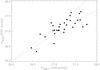 |
Fig. 5 m5007 for the F03 PN candidates (corrected for ~0.3 mag offset) plotted against the m5007 magnitudes measured in our survey. The dotted lines represent the 1σ uncertainty from the photometric errors of our survey. The two magnitude systems are consistent within the photometric errors with an offset that is constant with magnitude. |
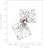 |
Fig. 6 Spatial distribution of PN candidates (black crosses). Red crosses represent objects classified as spurious after visual inspection. The magenta cross indicates the centre of M 87. Dotted ellipses trace the M 87 isophotes from R = 2.8 to R = 40.7′ along the photometric major axis, at a position angle PA = −25.6° (Kormendy et al. 2009). The solid squares depict our survey area. North is up, east to the left. |
We now investigate whether the PN number density profile follows the surface brightness profile of the galaxy light. On the basis of the simple stellar population theory, the luminosity-specific stellar death rate is insensitive to the population’s age, initial mass function, and metallicity (Renzini & Buzzoni 1986). Thus the probability of finding a PN at any location in a galaxy should be proportional to the surface brightness of the galaxy at that location.
In order to compare the surface brightness and PN number density profiles, we bin our PN sample in elliptical annuli, whose major axes are aligned with M 87′s photometric major axis and with ellipticities measured from the isophotes (see Fig. 6). We compute PN number densities as ratios between the number of PNs in each annulus and the area of the intersection of the annulus with our field of view. These areas, A(R), are estimated using a Monte Carlo integration technique.
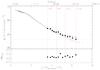 |
Fig. 7 Top panel: comparison between surface brightness profile from (Kormendy et al. 2009; crosses) and logarithmic PN number density profile of the emission line candidates, brighter than m5007 = 28.3, and corrected for spatial and colour incompleteness (open circles with error bars, see Table 4 for data), as function of the distance from the M 87 centre. The black dotted line represents the contribution of Lyα emission objects to the logarithmic PN number density profile, assuming a homogeneous distribution over the surveyed area. Under the same hypothesis, filled circles show the logarithmic PN number density profile when the Lyα contribution is statistically subtracted. Red lines mark the inner, intermediate and outermost regions of the M 87 halo (see text). Bottom panel: difference between the logarithmic PN number density profiles if we had used the automatically extracted sources without the final inspection: a value of zero would mean that no variation in the number of sources is implied in the annulus at a given radius. |
The PN number density profile must be corrected for spatial incompleteness because the
bright galaxy background and bright foreground stars may affect the detection of PNs. We
compute this completeness function, C(R), by adding a PN sample modelled
according to a Ciardullo et al. (1989) PNLF on the
scientific image. C(R) is then the fraction of simulated
objects recovered by Sextractor in the different elliptical annuli vs the input modelled
population, for PNs brighter than m5007 = 28.3 (values are
given in Table 4). The expected PN total number is
then: 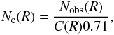 (4)where the value 0.71 accounts for the average
colour incompleteness (see Sect. 3.1.4). In Fig.
7 we show the comparison between the major axis
stellar surface brightness profile in the V band,
μK09 (Kormendy et al.
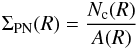
2009), and the PN logarithmic number density profile, defined as:
(4)where the value 0.71 accounts for the average
colour incompleteness (see Sect. 3.1.4). In Fig.
7 we show the comparison between the major axis
stellar surface brightness profile in the V band,
μK09 (Kormendy et al.
2009), and the PN logarithmic number density profile, defined as:  (5)where
 (6)is the PN number density corrected for
spatial and colour incompleteness, and μ0 is a constant value
added to match the PN number density profile to the μK09
surface brightness profile. In the same plot, we also indicate radii that select three
different regions in the halo of M 87; these regions are for
(6)is the PN number density corrected for
spatial and colour incompleteness, and μ0 is a constant value
added to match the PN number density profile to the μK09
surface brightness profile. In the same plot, we also indicate radii that select three
different regions in the halo of M 87; these regions are for
 ,
,
 and
and  ,
where
,
where  represents the mean distance of the PN sample from the centre of M 87. The innermost and
the outermost number density points are at radii R = 2.8′ and
R = 27.6′ respectively, and in Fig. 7 they are indicated with dotted red lines. The surface brightness and the
logarithmic PN number density profile agree well in the innermost region, they slightly
deviate in the intermediate region while in the outermost region the logarithmic PN number
density profile flattens. The difference between the two profiles amounts to 1.2 mag at
the outermost radii. This discrepancy would still be observed if we had used instead the
candidates from the automatic selection procedure without any final inspection: the
difference between the two number densities is too small to affect the slope at large
radii (see Fig. 7, bottom panel). We also note that
the flattening of the logarithmic number density profile is seen in both Suprime-Cam
fields independently.
represents the mean distance of the PN sample from the centre of M 87. The innermost and
the outermost number density points are at radii R = 2.8′ and
R = 27.6′ respectively, and in Fig. 7 they are indicated with dotted red lines. The surface brightness and the
logarithmic PN number density profile agree well in the innermost region, they slightly
deviate in the intermediate region while in the outermost region the logarithmic PN number
density profile flattens. The difference between the two profiles amounts to 1.2 mag at
the outermost radii. This discrepancy would still be observed if we had used instead the
candidates from the automatic selection procedure without any final inspection: the
difference between the two number densities is too small to affect the slope at large
radii (see Fig. 7, bottom panel). We also note that
the flattening of the logarithmic number density profile is seen in both Suprime-Cam
fields independently.
Empirically, the logarithmic PN number density profile follows light in elliptical (Coccato et al. 2009) and S0 (Cortesi et al. 2013) galaxies. However, these studies cover the halos out to typically only 20 kpc. The presence of Lyα background galaxies at z ~ 3.1 could also contribute to the flatter slope of the logarithmic PN number density profile, and so we need to evaluate their contribution to the number density at large radii. In Fig. 7 we show the contribution from Lyα contaminants (black dotted line) to the logarithmic number density (25% ± 5% of the total sample), assuming a homogeneous distribution in the surveyed area. We can make this assumption because the survey area 0.43 deg2 extends over many correlation lengths of the Lyα population at z = 3.14 (see Sect. 3.2).
Hence we can statistically subtract the contribution of the Lyα backgrounds objects from the number of PN candidates in each annulus and obtain the corrected number density profile (filled circles in Fig. 7). Now the error bars also account for the expected fluctuation of Lyα density (see Sect. 3.2 for details) and the flattening of the logarithmic PN number density profile is still observed. Using the derived α2.1 value for the halo from Sect. 4.4, the surface brightness profile translates to ~295 PNs down to m5007 = 28.3. Down to this magnitude our catalogue contains ~420 estimated PNs. The excess, then, is ~3.6 × σLyα, where σLyα is the standard deviation in the expected number of Lyα emitters from cosmic variance and Poisson statistics. Hence, the flattening can not be explained by fluctuations in the Lyα fraction. In what follows we investigate the physical origin of the flatter logarithmic PN number density profile.
4.2. The α parameter
The total number of PNs, NPN, is correlated with the total bolometric luminosity of the parent stellar population, Lbol, through the so-called α-parameter, that defines the luminosity-specific PN density: NPN = αLbol.
From stellar evolution theory it is found that the luminosity-specific stellar death rate
is insensitive to a stellar population’s age, initial mass function, and metallicity
(Renzini & Buzzoni 1986). Therefore, the
total number of PNs associated with a parent stellar population can be computed from the
bolometric luminosity using the formula: 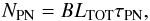 (7)where B is the specific
evolutionary flux (stars yrs-1
(7)where B is the specific
evolutionary flux (stars yrs-1 ), LTOT is the
total bolometric luminosity of the parent stellar population, and
τPN is the PN visibility lifetime. From Eq. (7), the luminosity-specific PN number,
α, is
), LTOT is the
total bolometric luminosity of the parent stellar population, and
τPN is the PN visibility lifetime. From Eq. (7), the luminosity-specific PN number,
α, is 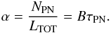 (8)Observed values of the α
parameter can then be interpreted as different values of τPN
for the PNs associated with different stellar populations, because variations of
B with metallicity or Initial Mass Function (IMF) slope are small
(Renzini & Buzzoni 1986).
(8)Observed values of the α
parameter can then be interpreted as different values of τPN
for the PNs associated with different stellar populations, because variations of
B with metallicity or Initial Mass Function (IMF) slope are small
(Renzini & Buzzoni 1986).
For any specific observation, the actual value of NPN depends
on the flux limit of the survey in which the PNs are detected. Hence, for our survey depth
we are interested in estimating α2.1, the number of PNs within
Δm = 2.1 magnitudes of the bright cutoff, per given amount of
bolometric luminosity emitted by the stellar population of the galaxy’s halo or ICL. For
any Δm, αΔm is defined such
that 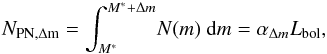 (9)where N(m)
is the PNLF and M∗ is the bright cutoff magnitude.
(9)where N(m)
is the PNLF and M∗ is the bright cutoff magnitude.
4.3. Halo and intracluster PN population
When studying the PN population in the outer region of M 87 out to 150 kpc from the galaxy’s centre, we expect contributions from the halo PNs and from ICPNs. The presence of ICL in cluster cores is a by-product of the mass assembly process of galaxy clusters (Murante et al. 2004, 2007).
The existence of intracluster PNs in Virgo has been demonstrated on the basis of extended imaging surveys in the 5007 Å [OIII] line (Feldmeier et al. 1998, 2003; Arnaboldi et al. 2002; Aguerri et al. 2005; Castro-Rodríguez et al. 2009) and spectroscopic follow-up (Arnaboldi et al. 1996, 2003, 2004). From the spectroscopic follow-up of Arnaboldi et al. (2004) we know the M 87 halo and the Virgo core ICL to coexist for distances R > 16′ from M 87’s centre (the FCJ field). In fact, the projected phase space diagram from Doherty et al. (2009) (PN line-of-sight velocity vs. radial distance from M 87 centre) shows the coexistence of the halo and ICL PN population out to 150 kpc.
To estimate the ICL luminosity in our two fields, we assume a constant surface brightness μV = 27.7 mag arcsec-2 (Mihos et al. 2005), and a V-band bolometric correction BCV = −0.85 (Buzzoni et al. 2006), which then gives a total bolometric luminosity in the ICL of LICL = 1.66 × 10¹⁰ L⊙ ,bol. This amounts to about one quoter of the bolometric luminosity of the M 87 halo.
4.4. Two component photometric model for M 87 halo and ICL, and determination of their α2.5 parameters
Therefore we now investigate whether the observed discrepancy between the logarithmic PN
number density profile and μV surface
brightness profile in Fig. 7 may be explained by
considering two PN populations associated with the M 87 halo and ICL. The physical
parameter that links a PN population to the luminosity of its parent stars is the
luminosity-specific PN number, the α parameter, thus a discrepancy
between μV and the measured logarithmic PN
number density profile may come from different α values for the halo and
ICL stellar population. This possibility is supported by Doherty et al. (2009) who measured two different values of α
for the bound (M 87 halo) and unbound (ICL) stellar component, which we are going to label
αhalo and αICL in what follows.
We can then define a photometric model with two components: ![Mathematical equation: \begin{eqnarray} \label{mod_sigma}\tilde{\Sigma}(R) &=& \left[\alpha_{2.1,\mathrm{halo}} {I}(R)_{\mathrm{halo,bol}} +\alpha_{2.1,\mathrm{ICL}} {I}_{\mathrm{ICL,bol}}\right] \\ \label{mod_sigma_ratio} &= &\alpha_{2.1,\mathrm{halo}} \left[ {I}(R)_{\mathrm{K09,bol}} +\left(\frac{\alpha_{2.1,\mathrm{ICL}}}{\alpha_{2.1,\mathrm{halo}}}-1\right) {I}_{\mathrm{ICL,bol}}\right] \end{eqnarray}](/articles/aa/full_html/2013/10/aa21652-13/aa21652-13-eq160.png) where
where  (R) represents the predicted PN surface
density in units of NPN pc-2,
I(R)halo and
IICL are the surface brightnesses for the halo and the ICL
components, and IK09 from Kormendy et al. (2009) is the observed total surface brightness from M 87 centre
out to 40′, accounting for both halo and ICL components. These surface brightnesses are in
units of L⊙ pc-2 and their bolometric values are
computed from the measured profiles in units of mag arcsec-2 via the formula:
(R) represents the predicted PN surface
density in units of NPN pc-2,
I(R)halo and
IICL are the surface brightnesses for the halo and the ICL
components, and IK09 from Kormendy et al. (2009) is the observed total surface brightness from M 87 centre
out to 40′, accounting for both halo and ICL components. These surface brightnesses are in
units of L⊙ pc-2 and their bolometric values are
computed from the measured profiles in units of mag arcsec-2 via the formula:
 where BCV = −0.85
and BC⊙ = −0.07 are the V-band and the Sun bolometric
corrections, and K = 26.4 mag arcsec-2 is a conversion factor
from mag arcsec-2 to physical units
L⊙ pc-2 in the V-band.
Assuming a fixed value of BCV = −0.85 for every galaxy type has a 10 per cent
internal accuracy, i.e. ±0.1 mag, for a range of simple stellar population (SSP) models
ranging from irregular to elliptical galaxies (Buzzoni
et al. 2006).
where BCV = −0.85
and BC⊙ = −0.07 are the V-band and the Sun bolometric
corrections, and K = 26.4 mag arcsec-2 is a conversion factor
from mag arcsec-2 to physical units
L⊙ pc-2 in the V-band.
Assuming a fixed value of BCV = −0.85 for every galaxy type has a 10 per cent
internal accuracy, i.e. ±0.1 mag, for a range of simple stellar population (SSP) models
ranging from irregular to elliptical galaxies (Buzzoni
et al. 2006).
The surface brightness profile can be expressed in terms of PN surface density
 :
:  (12)where μ0 is a
function of the α2.1,halo parameter:
(12)where μ0 is a
function of the α2.1,halo parameter:  (13)The value of μ0
is given by the value of the constant offset used in Eq. (5), and it can be fixed by fitting this offset between the observed
logarithmic PN surface density and the surface brightness profile,
μV, at smaller radii
(R ≤ 6.8′). From the fitted offset of
μ0 = 16.0 ± 0.1 mag arcsec-2, we compute the value
for α2.1,halo (Eq. (13)) resulting in
α2.1,halo = (0.63 ± 0.08) × 10-8 PN
(13)The value of μ0
is given by the value of the constant offset used in Eq. (5), and it can be fixed by fitting this offset between the observed
logarithmic PN surface density and the surface brightness profile,
μV, at smaller radii
(R ≤ 6.8′). From the fitted offset of
μ0 = 16.0 ± 0.1 mag arcsec-2, we compute the value
for α2.1,halo (Eq. (13)) resulting in
α2.1,halo = (0.63 ± 0.08) × 10-8 PN
 . The error on the determined
α2.1,halo is computed from the propagation of the errors on
the variables μ0 and BCV, the
latter having a 10% accuracy.
. The error on the determined
α2.1,halo is computed from the propagation of the errors on
the variables μ0 and BCV, the
latter having a 10% accuracy.
In Fig. 8 we show the fit of the two component PN
model to the observed PN logarithmic number density profile for
α2.1,ICL/α2.1,halo = 3 and a
constant ICL surface brightness of μICL = 27.7
mag arcsec-2 (Mihos et al. 2005). The
proposed model predicts a flatter slope for the PN logarithmic number density profile than
the slope of the V-band surface brightness profile
μV, as observed. The fitted value for
α2.1,ICL is then
α2.1,ICL = (1.89 ± 0.29) × 10-8 PN
.
Equation (11) shows explicitly that when α2.1,halo = α2.1,ICL then the logarithmic PN number density profile should closely follow light.
The measured values of α2.1,halo and α2.1,ICL correspond, down to the survey depth, to an estimated ~390 halo PNs, and ~310 ICPNs in the completeness-corrected sample, and to ~230 halo PNs and ~190 ICPNs in the observed sample.
To compute α2.5 for a PN sample which is not complete to
m∗ + 2.5, but only to a magnitude
mc < m∗ + 2.5, then
α2.5 is extrapolated by 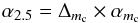 (14)where
  (15)If we use the derived M 87 PNLF (see Sect.
5) to compute the cumulative number of PNs
expected within 2.5 mag from the bright cut off, normalised to the cumulative number in
the first 2.1 mag, we obtain Δ2.1 ≃ 1.7. As a result, the predicted values of
α2.5, for the halo and ICL components are
(15)If we use the derived M 87 PNLF (see Sect.
5) to compute the cumulative number of PNs
expected within 2.5 mag from the bright cut off, normalised to the cumulative number in
the first 2.1 mag, we obtain Δ2.1 ≃ 1.7. As a result, the predicted values of
α2.5, for the halo and ICL components are
 and
and
 . The errors on the
α2.5 values also take the uncertainty on the magnitude of
the bright cutoff into account.
. The errors on the
α2.5 values also take the uncertainty on the magnitude of
the bright cutoff into account.
 |
Fig. 8 As in the top panel of Fig. 7 but with the modelled surface brightness profile from the two component photometric model superposed (dot-dashed black line). This modelled profile reproduces the flattening observed in the logarithmic number density well. |
4.5. Comparison with previously determined α2.5 values
The α2.5 values for the M 87 halo and ICL were measured in previous works by Durrell et al. (2002) and Doherty et al. (2009). There are several assumptions that are made when computing these values, hence is important to address them before the actual numbers are compared. As already pointed out in the previous section, when α2.5 is computed for a PN sample which is not complete to m∗ + 2.5, then α2.5 is extrapolated by following Eq. (14).
In the studies of Durrell et al. (2002) and Doherty et al. (2009), the PN samples were complete one magnitude down the bright cutoff of the PNLF. Then, α2.5 was computed using the extrapolation on the basis of the analytic formula for N(m) by Ciardullo et al. (1989).
In Sect. 5 we derive the M 87 PNLF in the brightest 2.5 mag range, which shows a steeper slope at ~1.5 mag below the cutoff than what is predicted by the analytical formula. If we use the observed PNLF then the cumulative number of PNs expected within 2.5 mag from the bright cut off, normalised to the cumulative number in the first magnitude, is about 2.7 times that predicted by the analytical PNLF. When comparing the actual values for the α2.5 measured by Durrell et al. (2002) and Doherty et al. (2009), they need to be rescaled by this fraction.
In the current work and in Doherty et al. (2009),
α2.5 values were measured for the halo and ICL separately,
using only the PNs associated with each component. In Doherty et al. (2009) the line-of-sight velocity of each PN was used to tag the
PN candidate as M 87 halo or ICL. In Durrell et al.
(2002) this information was not available. Following Doherty et al. (2009), only 58% of the PN candidates considered by
Durrell et al. (2002) are truly ICL. When this
correction is applied, then the value measured by Durrell
et al. (2002) for the ICPNs is
α2.5,ICL = 1.3 × 10⁻⁸ PN
. If in addition we correct this
α2.5 value for the ICL for the different shape of the PNLF,
we get α2.5,ICL,DU02 = 3.6 × 10⁻⁸ PN
. This value is ~10% greater than
ours, but consistent within the uncertainties and the contamination from continuum sources
in the F03 catalogue (see Sect. 3.3).
When we correct the α2.5 values for halo and ICL from Doherty et al. (2009) by a factor 2.7, we obtain
α2.5,halo,D09 = 8.4 × 10⁻⁹ PN
and
α2.5,ICL,D09 = 1.9 × 10⁻⁸ PN
. These values are smaller than ours, but
consistent within the uncertainties and the colour/detection completeness corrections made
here (see Sect. 4.1) but not in Doherty et al. (2009).
4.6. Implications of the measured α2.5 values
According to the analytical formula of Ciardullo et al.
(1989) for the PNLF, α2.5 equals ~1/10 of the
total luminosity-specific PN number α (see also Buzzoni et al. 2006), assuming that PNs are visible down to 8 mags from
the bright cutoff (Ciardullo et al. 1989). If we
use this analytical function to extrapolate the total number of PNs from 2.5 to 8 mag
below the bright cutoff our measured values for α2.5 translate
to total luminosity-specific PN numbers for the two components of
αhalo = 1.1 × 10⁻⁷ PN
and
αICL = 3.3 × 10⁻⁷ PN
. We can recast these numbers in terms of
the PN visibility lifetime τPN through Eq. (8), assuming
 yr-1 (Buzzoni et al. 2006). τPN is then
≃6.1 × 10³ yr and ≃18.3 × 10³ yr for the M 87 halo and ICL PNs.
Note, that these would be lower limits, because at this stage we do not know whether the
extrapolation from 2.5 mag below the cutoff to fainter magnitudes follows the analytical
formula, or whether it is steeper.
yr-1 (Buzzoni et al. 2006). τPN is then
≃6.1 × 10³ yr and ≃18.3 × 10³ yr for the M 87 halo and ICL PNs.
Note, that these would be lower limits, because at this stage we do not know whether the
extrapolation from 2.5 mag below the cutoff to fainter magnitudes follows the analytical
formula, or whether it is steeper.
Observationally there is some evidence that α is on average larger for bluer systems (Peimbert 1990; Hui et al. 1993). The measurements of the colour profile in M 87 show a bluer gradient towards larger radii (Liu et al. 2005; Rudick et al. 2010): a fit of the colour profile along the major axis inside 1000″ has a slope of –0.11 in Δ(B − V)/Δlog (R) (Rudick et al. 2010). The observed PN logarithmic number density profile measured in this work is consistent with the empirical result of a gradient towards bluer colours at large radii. In the proposed model, the gradient is caused by the increased contribution of ICL at large radii, which is bluer than the M 87 halo population.
One can ask whether the metallicity of the parent stellar population may influence the number of PNs associated with a given bolometric luminosity. We are interested in population effects in the advanced evolutionary phases of stellar evolution, as the [OIII] 5007 Å emission and its line width are weakly dependent on the chemical composition of the nebula (Dopita et al. 1992; Schönberner et al. 2010). For stellar populations with the same IMF and ages, Weiss & Ferguson (2009) computed models for the asymptotic giant branch (AGB) for stars between 1.0 and 6.0 M⊙ with different metallicities. Their results show that the number of AGB stars varies with the chemical composition, because the latter effects the lifetime on the thermally pulsing AGB, with the longest lifetime obtained for metallicity between half and one tenth of Z⊙. Given that the evolutionary path followed by a star from the end of the AGB to the beginning of the cooling phase of the central white dwarf corresponds to the planetary nebulae phase, it is suggestive to infer that stellar populations with metallicity –0.5 to –0.1 solar may have a larger number of PNs than stellar populations with solar metallicity or higher, for the same bolometric luminosity. The metallicities of ICL stars in the Virgo cluster core were measured by Williams et al. (2007) using colour magnitude diagrams to be between –0.5 to –0.1 solar. If the stars in the M 87 halo have a higher metallicity, we might expect a variation of the luminosity specific PN number in the region of radii where the M 87 stellar halo and the ICL are superposed along the line-of-sight (Doherty et al. 2009), as is quantified for the first time in this work.
5. Planetary nebula luminosity function in the outer regions of M 87
5.1. PNLF
We can now use our large PN sample in the outer regions of M 87 to investigate the properties of the PNLF. To do this we need to take into account that the fraction of detected PNs on our scientific images can be affected by incompleteness, and that this incompleteness is a function of magnitude.
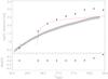 |
Fig. 9 Top panel: luminosity function of the selected PNs in the outer regions of M 87, corrected for colour and detection incompleteness. The error bars show the 1σ uncertainty from counting statistics. Data are binned into 0.3 mag intervals (see Table 5 for numerical values). The solid red line represents the analytical PNLF model for a distance modulus of 30.8, convolved with photometric errors. The black line shows the Lyα LF from Gronwall et al. (2007), scaled to the effective surveyed volume of the M 87 SUB1 and M 87 SUB2 fields, with the shaded area showing the cosmic variance due to Lyα density fluctuations (~20%, see Sect. 3.2). Bottom panel: difference between the PNLF if we had used instead the automatically extracted sources without any final inspection. This plot shows that spurious detections affect mostly the two faintest magnitude bins. |
As for the spatial completeness, we quantify this effect by adding a modelled sample of
PNs on the scientific images and computing the fraction recovered by Sextractor of this
input simulated PN population as function of magnitude (see Table 5 for values). In Fig. 9 we show
the PNLF for the extracted candidates corrected for colour and detection incompleteness.
We can compare this PNLF with the analytical formula by Ciardullo et al. (1989) (16)where c1 is a
normalisation constant, c2 = 0.307 and
M∗(5007) = −4.51 mag is the absolute magnitude of the PNLF
bright cutoff (Ciardullo et al. 1989). In Fig.
9 the red solid line shows the prediction from the
analytical formula for a distance modulus of 30.8, after convolution with photometric
errors and normalisation to the brightest observed bins. The comparison of the derived
PNLF with the analytical formula shows two differences. First we detect one object with a
m5007 = 25.7 that is ~0.6 mag brighter than the
expected cutoff for a distance modulus of 30.8. Second we measure a slope in the PNLF at
~1.5 mag below the cutoff that is steeper than what is predicted by the analytical
formula in this magnitude range (Ciardullo et al.
1989; Henize & Westerlund 1963).
(16)where c1 is a
normalisation constant, c2 = 0.307 and
M∗(5007) = −4.51 mag is the absolute magnitude of the PNLF
bright cutoff (Ciardullo et al. 1989). In Fig.
9 the red solid line shows the prediction from the
analytical formula for a distance modulus of 30.8, after convolution with photometric
errors and normalisation to the brightest observed bins. The comparison of the derived
PNLF with the analytical formula shows two differences. First we detect one object with a
m5007 = 25.7 that is ~0.6 mag brighter than the
expected cutoff for a distance modulus of 30.8. Second we measure a slope in the PNLF at
~1.5 mag below the cutoff that is steeper than what is predicted by the analytical
formula in this magnitude range (Ciardullo et al.
1989; Henize & Westerlund 1963).
We discuss the significance of these deviations in turn.
Over-luminous source
– Figure 9 also shows the comparison of the PNLF from our PN sample with the Lyα LF from Gronwall et al. (2007), scaled to our effective surveyed volume. The hatched range gives the uncertainty in the latter. We see that the bright end of the Lyα LF is consistent with the luminosity of the over-luminous object, within the photometric errors. Earlier suggestions that such overluminous objects could be due to a depth effect from Virgo ICL (Jacoby et al. 1990, C98) are not consistent with more recent studies of the ICL in Virgo; see Sect. 5.4. To definitively resolve the question of the nature of this object, whether it is a Lyα emitter or an object in the M 87 halo, requires spectroscopic follow-up.
Steeper PNLF 1.5 mag below the bright cutoff
– First, we carried out a Kolmogorov-Smirnov test to check whether our empirical PNLF can be drawn from the Ciardullo et al. (1989) analytical function, and this possibility is rejected. Next, because our sample covers 0.5° in the M 87 halo, we can investigate the radial variation of the PNLF out to radii of 30′. We compute the PNLF for each of the three PN subsamples associated with the radial bins described in Sect. 4.1, correcting for colour and detection incompleteness, and subtracting the respective contribution from Lyα background objects. These are shown in the upper panel of Fig. 10, where the error bars also account for ~20% cosmic variance in the Lyα density (see Sect. 3.2). We then compare the three PNLFs after normalisation to the total number of objects in each radial bin and carry out a Kolmogorov-Smirnov test to check whether they can result from the same underlying distribution. The probability that these three PNLFs are extracted from the same distribution is high, PKS > 99%.
These results are significant because the steepening of the PNLF is thus shown to be present in all three radial bins, while we know that the ICPN population contributes mostly to the outermost bin, see discussion in Sect. 4.3, and that any residual contamination of Lyα background emitters is also largest in the outermost radial region. We also checked that the PNLFs in the two Suprime-Cam fields are similar; both show the steepening at faint magnitudes. Hence we must conclude that the observed steepening of the PNLF is an intrinsic property of the PN population (halo and ICL) in the outer regions of M 87.
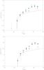 |
Fig. 10 Top panel: empirical PNLFs in three radial ranges corrected for colour and detection incompleteness: PN candidates within 6.5′ from M 87 centre – triangles, PN candidates between 6.5′ and 13.5′ from M 87 centre – diamonds, PN candidates in the outermost region (distances greater than 13.5′) – squares.The respective Lyα contribution expected in each radial bin was subtracted. Magnitudes are binned in 0.3 mag bins and the error bars represent the 1σ uncertainty from counting statistics combined with the uncertainty from cosmic variance in the Lyα density (see text for details). As before, the red solid line is the convolved analytical formula of Ciardullo et al. (1989) for distance modulus 30.8. Lower panel: same as for the upper plot, but now the three PNLFs are normalised at the total number of objects in each radial bin. The three data sets are consistent with being drawn from the same underlying distribution. |
 |
Fig. 11 Completeness-corrected PNLF for the M 87 halo (full dots) with magnitudes binned in 0.2 mag bins; error bars include Poisson statistics and 20% variance in the number of subtracted Lyα contaminants. The continuous line indicates the resulting fit of the generalised analytical formula Eq. (16), for the values of the free parameters given by c1 = 2017.2, c2 = 1.17 and a distance modulus of m − M = 30.74. The generalised PNLF is convolved with the photometric errors. |
5.2. Generalised analytical model for the PNLF and distance modulus of M 87 halo
We determine the PNLF for the M 87 halo as follows. From the colour and detection
corrected PNLF, shown in the top panel of Fig. 9, we
subtract the expected contribution from Lyα emitters. Using the measured
values of α2.5 for the M 87 halo and ICL PN population, we
derive the fraction of PN in the M 87 halo, using
 (17)where
LICL, LLhalo
are given in Table 3 and
α2.5,ICL/α2.5,halo = 3. We show
the PNLF of the halo of M 87 in Fig. 11; error bars
include Poisson statistics and a 20% cosmic variance of the Lyα density.
(17)where
LICL, LLhalo
are given in Table 3 and
α2.5,ICL/α2.5,halo = 3. We show
the PNLF of the halo of M 87 in Fig. 11; error bars
include Poisson statistics and a 20% cosmic variance of the Lyα density.
We now attempt to fit this PNLF with a generalised version of the analytical formula reported in Eq. (16). We continue to assume that the bright cutoff near M∗ is invariant for different PN populations, but we now allow for a free faint-end slope parameter c2, in addition to varying the parameter c1 equivalent to sample size. For the fit to the data we use robust non-linear least squares curve fitting, i.e., the IDL routine mpfit (Markwardt 2009), and account for the photometric errors. We derive the following values for the free parameters: c1 = 2017.2, c2 = 1.17 and m∗ = 26.23, for a reduced χ2 = 1.01. Figure 11 shows that this model is an excellent fit to the empirical PNLF for the halo of M 87.
The fitted value of m∗ = 26.23 corresponds to a nominal distance modulus for M 87 of m − M = 30.74 mag, or D = 14.1 Mpc. Since the generalised PNLF formula has not been calibrated and our candidates are not spectroscopically confirmed, we regard this as preliminary and do not give an error on m − M. This value for the distance modulus is ~0.4 mag brighter than that measured with the surface brightness fluctuation method, 31.18 ± 0.07 mag (Mei et al. 2007), and with the tip of the red giant branch, 31.12 ± 0.14 mag (Bird et al. 2010), which correspond to distances of 17.2 ± 0.5 Mpc and 16.7 ± 0.9 Mpc.
Properties of the stellar populations in the bulge of M 31 and in the halo of M 87.
5.3. Comparison of the PNLF in the M 87 halo and in the M 31 bulge
Here we compare the observed properties of the PNLF in M 87 with the PNLF in the M 31 bulge which was used to calibrate the analytical formula by C98. The PN population of the M 31 bulge was studied in detail by Ciardullo et al. (1989); it has similar depth to our PNLF, i.e. it is complete 2.5 mag down the bright cutoff of the PNLF. Also, the stellar population in the M 31 has similar metallicity, colour and stellar population age as the population in the inner ~6′ of M 87; see Table 3 for a complete list of the parameters.
We take the PN samples for M 31 and the halo of M 87 and normalise them by the sampled luminosity, then correct for the distance modulus. The results are shown in Fig. 12, where the PNLF for the halo of M 87 is shown before and after the subtraction of Lyα contaminants. For the points where the Lyα contribution is subtracted the error bars take a ~20% cosmic variance of the Lyα density (see Sect. 3.2) into account. Within 1 mag of the bright cutoff, the M 87 PN population has fewer PNs than the PNLF of M 31, i.e., the slope of the PNLF for the halo of M 87 is steeper towards fainter magnitudes.
In old stellar populations, one expects the PN central stars to be dominated by low mass cores Mcore ≤ 0.55 M⊙. Thus it is plausible that the slope of the PNLF should be steeper than predicted by modelling the fading of a uniformly expanding homogeneous gas sphere ionised by a non-evolving star in a single PN (Henize & Westerlund 1963). The comparison between the PNLFs of M 87 and M 31 may indicate that the M 87 halo hosts a stellar population with a larger fraction of low mass cores with respect to the M 31 bulge.
From observations, there is further evidence that the faint end slope of the luminosity function may depend on the parent stellar population. Ciardullo et al. (2004) reported that star-forming systems, like the disk of M 33 and the Small Magellanic Cloud (SMC), have shallower slopes ~1.5 mags below the bright cutoff when compared to older stellar populations such as NGC 5128 or M 31. These shallower slopes correspond to lower values of c2 in Eq. (16).
5.4. Comparison with previous PNLF distance measurements for M 87
We already referred in Sect. 3.3 to the work of C98 who carried out a PN survey in an area of 16′ × 16′ centred on M 87, and investigated the properties of the PNLF. F03 studied the properties of ICPNs in the Virgo ICL, including an area of 16′ × 16′ centred 14.8′ north of M 87. Both surveys overlap with our current survey, but have a constant zero point offset Δ = 0.3 mag relative to our measured magnitudes (see discussion in Sect. 3.3).
Figure 13 compares the PNLFs of the matched subsamples common to our catalogue and those of C98 and F03, respectively. A residual zero point offset Δ = 0.3 mag has been applied to the C98 and F03 subsamples. With this zero point shift, the empirical PNLFs agree very well within one magnitude of the bright cutoff, and are consistent with a distance modulus of 30.8. Without the zero point shift, the distance modulus obtained from the PNLFs of C98 and F03 would be 30.5. Thus the value obtained for our new M 87 halo PN sample (30.75), which is closer to other determinations (Sect. 5.2), indicates a systematic effect in the C98, F03 photometry, in the sense of brighter m5007 in these samples. This systematic effect can explain and resolve some of the tension between the assumptions and results of C98, F03, and more recent findings on the spatial distribution of ICPNs in the Virgo cluster and the radial extension of the M 87 halo, as discussed now.
C98 find that their empirical PNLF deviates from the analytical formula and link the deviations with the presence of an ICPN population uniformly distributed in the Virgo cluster volume. C98 assume that all PNs at distances larger than Riso > 4.8′ from the centre of M 87 are ICPNs. Fitting a PNLF to this component, they derive that the ICPN population must extend 4 Mpc in front of M 87; see Fig. 8 and its figure caption in C98 for further details. The depth effect, which is equivalent to a brightening of the PNLF by foreground ICPNs, places the near edge of the ICL population at a distance modulus of 30.3, corresponding to a distance of 11 Mpc.
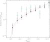 |
Fig. 12 Luminosity-normalised PNLFs for the bulge of M 31 (triangles) and the halo of M 87 (circles). Open circles and filled circles represent, respectively, the PNLF of the halo of M 87 before and after subtraction of the expected number of Lyα contaminants in each bin. Data are binned into 0.25 mag intervals. M 87 has a higher number of faint PNs per unit bolometric luminosity and its PNLF has a steeper slope towards faint magnitudes than M 31. |
The assumptions of C98 on the membership of PNe at Riso > 4.8′ from M 87 to the ICL and on the spatial distribution of the ICL are not supported by the results of the spectroscopic follow-up of Arnaboldi et al. (2004) and the wide area ICPN survey by Castro-Rodríguez et al. (2009). The spectroscopic follow-up by Arnaboldi et al. (2004) showed that in the FCJ field of F03 at 14.8′ from the M 87 centre 87% of the PNs are bound to the M 87 halo, and only 13% are ICPNs. Thus the fraction of ICPNs in regions that are even closer to the centre, as in the C98 Riso > 4.8′, sample, will be down to a few %. The wide area survey for ICPNs carried out by Castro-Rodríguez et al. (2009) shows that the ICL is associated with only the densest regions of the Virgo cluster, ~0.4 Mpc around M 87. Hence the brightening of the PNLF expected due to foreground ICPNs is <0.1 mag. These results indicate that the C98 PNs at Riso > 4.8′ are bound to the M 87 halo, with very limited contamination by ICL: thus they are at the distance of M 87 and the brightening of the C98 sample is not caused by volume effects or a contamination by ICPNs. Similar arguments apply to the F03 PN sample.
We therefore conclude that the magnitudes for the C98, F03 PNs sample must be systematically too bright by 0.3 mag, and that our new photometry is reliable.
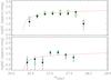 |
Fig. 13 Luminosity functions of the matched PN samples from this survey (filled circles), from C98 (top panel, green squares), and from F03 (bottom panel, cyan triangles). The error bars show the 1σ uncertainty from counting statistics. Data are binned into 0.2 mag intervals. The solid red line represents the analytical PNLF model using a distance modulus of 30.8, convolved with photometric errors. The magnitude range is driven by the magnitude limit of the C98 sample (top panel) and F03 sample (bottom panel). A zero point shift Δ = 0.3 mag relative to our sample was applied to both survey. |
6. Summary and conclusions
We carried out a deep survey for planetary nebulas (PNs) in two wide fields of 34′× 27′, covering the halo of the cD galaxy NGC 4486 (M 87) in the Virgo cluster with Suprime-Cam at the Subaru telescope. Both fields were imaged through a narrow-band filter centred at the redshifted [OIII]λ5007 Å emission and a broad-band V filter. The surveyed area covers the halo of M 87 out to a radial distance of 150 kpc. This is the largest survey so far for PNs in the M 87 halo in terms of number of detected PN candidates, depth and area coverage.
PN candidates were identified via the on-off band technique on the basis of automatic selection criteria using their narrow-band colours and their two-dimensional light distributions. The final photometric catalogue contains 688 objects, with a magnitude range extending from the apparent magnitude of the bright cutoff at Virgo distance down to 2.2 mag deeper.
We studied the radial number density profile of the PN candidates and compared it with the V-band surface brightness profile of the stellar light in the M 87 halo. The logarithmic PN number density profile shows good agreement with the μV surface brightness profile within 13′ from M 87’s centre, but flattens at large radii. At the most distant point the difference to the prediction from the light profile is 1.2 mags. We investigated whether contributions from background Lyα emitters at redshift z = 3.1 can be responsible for the flatter distribution. By using the Lyα LF from Gronwall et al. (2007) scaled to our effective surveyed volume, we constrained the Lyα contribution to be 25% ± 5% of the total sample over the whole surveyed area, and we concluded that it cannot explain the factor 3 more sources in the outer regions that are responsible for the flatter profile.
Stimulated by the early finding of Doherty et al.
(2009) who determined different luminosity specific PN numbers for the M 87 halo
light and the ICL, we propose a two component model for the PN population, with the ICL
contributing a larger number of PNs per unit light. This composite model is consistent with
the observed flattening of the logarithmic PN density profile when the luminosity specific
PN numbers are  and
and  , for the M 87 halo and ICL population
respectively.
, for the M 87 halo and ICL population
respectively.
Because of the large magnitude range of this PN survey, we were able to study the shape of the PNLF in detail and measured a steeper slope at faint magnitudes than what is expected from the analytical formula of Ciardullo et al. (1989). The fit of the generalised PNLF formula (Eq. (16)) to the empirical PNLF of the M 87 halo population gives faint-end slope of c2 = 1.17 and a nominal distance modulus of 30.74.
The depth of the current survey allowed us to carry out a comparison with the benchmark for PNLF studies, the M 31 bulge. The comparison of the M 87 halo PNLF with the M 31 bulge PNLF, when both are normalised by the sampled bolometric luminosity, shows that the former has fewer PNs at bright magnitudes, and a steeper slope towards the faint end. The steepening of the PNLF at fainter magnitudes is consistent with a larger fraction of PNs with low mass cores. PN evolution models and stellar population measurements at large radii will be needed to understand the stellar population effects that shape the PNLF of the M 87 halo.
Online material
Number density and logarithm number density profile for the colour and spatial corrected sample of emission line objects.
PNLF for the colour and detection corrected sample of emission line objects.
Dark sky is an image of an empty field (off target) on the sky.
The reference [OIII] and V-band exposures are the one used as reference images for the final image combination.
IRAF is distributed by the National Optical Astronomy Observatory, which is operated by the Association of Universities for Research in Astronomy (AURA) under cooperative agreement with the National Science Foundation.
The astrometry accuracy of the [OIII] frames was improved by using the corresponding V-band image plate solution after being registered to the V-band image coordinate system. On/off images need to be registered on the same system due to the selection of PNs via colour excess (see Sect. 3.1).
These values of Z[OIII] and Z[V] are consistent with those obtained by Castro-Rodríguez et al. (2009) where they analyze data collected with the Suprime-Cam at the Subaru telescope through the same filters: [OIII] narrow-band filter (λc = 5029 Å Δλ = 74 Å), and broad-band V-filter (λc = 5500 Å Δλ = 956 Å).
In these simulations we adopted a Moffat β = 2.5 profile to define the PSF of unresolved sources (see Sect. 2.2 for details) and an exponential LF similar to the one describing the PNLF in Ciardullo et al. (1998).
This area does not include the regions affected by high background noise and bad pixels (see Sect. 3.1.3).
Acknowledgments
We thank the on-site Subaru staff for their support and A. Aguerri and N. Castro-Rodriguez for helping with the routines that were used for the PNs catalogue extraction. We are also thankful to G. Bono and A. Weiss for helpful discussions on stellar evolution in the AGB phase, and to the referee for her/his comments which improved the paper. A.L. thanks J. Elliott, B. Agarwal and G. Avvisati for the support and helpful comments on the paper. M.A.R. would like to thank F. Makata for support in using the Suprime-Cam Data Reduction (sdfred) pipeline. L.C. acknowledges funding from the European Community’s Seventh Framework Programme (FP7/2007-2013/) under grant agreement No. 229517. This research has made use of the 2MASS catalogue data.
References
- Aguerri, J. A. L., Gerhard, O. E., Arnaboldi, M., et al. 2005, AJ, 129, 2585 [NASA ADS] [CrossRef] [Google Scholar]
- Arnaboldi, M., Freeman, K. C., Mendez, R. H., et al. 1996, ApJ, 472, 145 [NASA ADS] [CrossRef] [Google Scholar]
- Arnaboldi, M., Aguerri, J. A. L., Napolitano, N. R., et al. 2002, AJ, 123, 760 [NASA ADS] [CrossRef] [Google Scholar]
- Arnaboldi, M., Freeman, K. C., Okamura, S., et al. 2003, AJ, 125, 514 [NASA ADS] [CrossRef] [Google Scholar]
- Arnaboldi, M., Gerhard, O., Aguerri, J. A. L., et al. 2004, ApJ, 614, L33 [NASA ADS] [CrossRef] [Google Scholar]
- Bertin, E., & Arnouts, S. 1996, A&AS, 117, 393 [NASA ADS] [CrossRef] [EDP Sciences] [Google Scholar]
- Binggeli, B., Tammann, G. A., & Sandage, A. 1987, AJ, 94, 251 [NASA ADS] [CrossRef] [Google Scholar]
- Bird, S., Harris, W. E., Blakeslee, J. P., & Flynn, C. 2010, A&A, 524, A71 [NASA ADS] [CrossRef] [EDP Sciences] [Google Scholar]
- Buton, C., Copin, Y., Aldering, G., et al. 2013, A&A, 549, A8 [NASA ADS] [CrossRef] [EDP Sciences] [Google Scholar]
- Buzzoni, A., Arnaboldi, M., & Corradi, R. L. M. 2006, MNRAS, 368, 877 [NASA ADS] [CrossRef] [Google Scholar]
- Castro-Rodríguez, N., Aguerri, J. A. L., Arnaboldi, M., et al. 2003, A&A, 405, 803 [NASA ADS] [CrossRef] [EDP Sciences] [Google Scholar]
- Castro-Rodríguez, N., Arnaboldi, M., Aguerri, J. A. L., et al. 2009, A&A, 507, 621 [NASA ADS] [CrossRef] [EDP Sciences] [Google Scholar]
- Ciardullo, R. 2010, PASA, 27, 149 [NASA ADS] [Google Scholar]
- Ciardullo, R., Jacoby, G. H., Ford, H. C., & Neill, J. D. 1989, ApJ, 339, 53 [NASA ADS] [CrossRef] [Google Scholar]
- Ciardullo, R., Jacoby, G. H., Feldmeier, J. J., & Bartlett, R. E. 1998, ApJ, 492, 62 [NASA ADS] [CrossRef] [Google Scholar]
- Ciardullo, R., Durrell, P. R., Laychak, M. B., et al. 2004, ApJ, 614, 167 [Google Scholar]
- Coccato, L., Gerhard, O., Arnaboldi, M., et al. 2009, MNRAS, 394, 1249 [NASA ADS] [CrossRef] [Google Scholar]
- Colless, M., Ellis, R. S., Taylor, K., & Hook, R. N. 1990, MNRAS, 244, 408 [NASA ADS] [Google Scholar]
- Cortesi, A., Arnaboldi, M., Coccato, L., et al. 2013, A&A, 549, A115 [NASA ADS] [CrossRef] [EDP Sciences] [Google Scholar]
- Doherty, M., Arnaboldi, M., Das, P., et al. 2009, A&A, 502, 771 [NASA ADS] [CrossRef] [EDP Sciences] [Google Scholar]
- Dopita, M. A., Jacoby, G. H., & Vassiliadis, E. 1992, ApJ, 389, 27 [NASA ADS] [CrossRef] [Google Scholar]
- Durrell, P. R., Ciardullo, R., Feldmeier, J. J., Jacoby, G. H., & Sigurdsson, S. 2002, ApJ, 570, 119 [NASA ADS] [CrossRef] [Google Scholar]
- Feldmeier, J. J., Ciardullo, R., & Jacoby, G. H. 1998, ApJ, 503, 109 [NASA ADS] [CrossRef] [Google Scholar]
- Feldmeier, J. J., Ciardullo, R., Jacoby, G. H., & Durrell, P. R. 2003, ApJS, 145, 65 [NASA ADS] [CrossRef] [Google Scholar]
- Feldmeier, J. J., Ciardullo, R., Jacoby, G. H., & Durrell, P. R. 2004, ApJ, 615, 196 [NASA ADS] [CrossRef] [Google Scholar]
- Gawiser, E., Francke, H., Lai, K., et al. 2007, ApJ, 671, 278 [NASA ADS] [CrossRef] [Google Scholar]
- Gerhard, O., Arnaboldi, M., Freeman, K. C., et al. 2005, ApJ, 621, L93 [NASA ADS] [CrossRef] [Google Scholar]
- Gronwall, C., Ciardullo, R., Hickey, T., et al. 2007, ApJ, 667, 79 [NASA ADS] [CrossRef] [Google Scholar]
- Hammer, F., Flores, H., Lilly, S. J., et al. 1997, ApJ, 481, 49 [CrossRef] [Google Scholar]
- Henize, K. G., & Westerlund, B. E. 1963, ApJ, 137, 747 [NASA ADS] [CrossRef] [Google Scholar]
- Hogg, D. W. 1999 [arXiv:astro-ph/9905116] [Google Scholar]
- Hogg, D. W., Cohen, J. G., Blandford, R., & Pahre, M. A. 1998, ApJ, 504, 622 [NASA ADS] [CrossRef] [Google Scholar]
- Hui, X., Ford, H. C., Ciardullo, R., & Jacoby, G. H. 1993, ApJ, 414, 463 [NASA ADS] [CrossRef] [Google Scholar]
- Jacoby, G. H. 1989, ApJ, 339, 39 [NASA ADS] [CrossRef] [Google Scholar]
- Jacoby, G. H., Africano, J. L., & Quigley, R. J. 1987, PASP, 99, 672 [NASA ADS] [CrossRef] [Google Scholar]
- Jacoby, G. H., Ciardullo, R., & Ford, H. C. 1990, ApJ, 356, 332 [NASA ADS] [CrossRef] [Google Scholar]
- Kormendy, J., Fisher, D. B., Cornell, M. E., & Bender, R. 2009, ApJS, 182, 216 [NASA ADS] [CrossRef] [Google Scholar]
- Liu, Y., Zhou, X., Ma, J., et al. 2005, AJ, 129, 2628 [NASA ADS] [CrossRef] [Google Scholar]
- Markwardt, C. B. 2009, in Astronomical Data Analysis Software and Systems XVIII, eds. D. A. Bohlender, D. Durand, & P. Dowler, ASP Conf. Ser., 411, 251 [Google Scholar]
- Mei, S., Blakeslee, J. P., Côté, P., et al. 2007, ApJ, 655, 144 [NASA ADS] [CrossRef] [Google Scholar]
- Méndez, R. H., Kudritzki, R. P., Ciardullo, R., & Jacoby, G. H. 1993, A&A, 275, 534 [NASA ADS] [Google Scholar]
- Méndez, R. H., Teodorescu, A. M., Schönberner, D., Jacob, R., & Steffen, M. 2008, ApJ, 681, 325 [NASA ADS] [CrossRef] [Google Scholar]
- Merrett, H. R., Merrifield, M. R., Douglas, N. G., et al. 2006, MNRAS, 369, 120 [NASA ADS] [CrossRef] [Google Scholar]
- Mihos, J. C., Harding, P., Feldmeier, J., & Morrison, H. 2005, ApJ, 631, L41 [NASA ADS] [CrossRef] [Google Scholar]
- Miyazaki, S., Komiyama, Y., Sekiguchi, M., et al. 2002, PASJ, 54, 833 [NASA ADS] [CrossRef] [Google Scholar]
- Murante, G., Arnaboldi, M., Gerhard, O., et al. 2004, ApJ, 607, L83 [NASA ADS] [CrossRef] [Google Scholar]
- Murante, G., Giovalli, M., Gerhard, O., et al. 2007, MNRAS, 377, 2 [Google Scholar]
- Peimbert, M. 1990, Rev. Mex. Astron. Astrofis., 20, 119 [NASA ADS] [Google Scholar]
- Peng, E. W., Ford, H. C., & Freeman, K. C. 2004, ApJ, 602, 685 [NASA ADS] [CrossRef] [Google Scholar]
- Renzini, A., & Buzzoni, A. 1986, in Spectral Evolution of Galaxies, eds. C. Chiosi, & A. Renzini, Astrophys. Space Sci. Lib., 122, 195 [Google Scholar]
- Rudick, C. S., Mihos, J. C., Harding, P., et al. 2010, ApJ, 720, 569 [NASA ADS] [CrossRef] [Google Scholar]
- Saglia, R. P., Fabricius, M., Bender, R., et al. 2010, A&A, 509, A61 [NASA ADS] [CrossRef] [EDP Sciences] [Google Scholar]
- Schönberner, D., Jacob, R., Sandin, C., & Steffen, M. 2010, A&A, 523, A86 [NASA ADS] [CrossRef] [EDP Sciences] [Google Scholar]
- Somerville, R. S., Lee, K., Ferguson, H. C., et al. 2004, ApJ, 600, L171 [NASA ADS] [CrossRef] [Google Scholar]
- Teplitz, H. I., Malkan, M. A., Steidel, C. C., et al. 2000, ApJ, 542, 18 [NASA ADS] [CrossRef] [Google Scholar]
- Theuns, T., & Warren, S. J. 1997, MNRAS, 284, L11 [CrossRef] [Google Scholar]
- van Dokkum, P. G. 2001, PASP, 113, 1420 [NASA ADS] [CrossRef] [Google Scholar]
- Ventimiglia, G., Arnaboldi, M., & Gerhard, O. 2011, A&A, 528, A24 [NASA ADS] [CrossRef] [EDP Sciences] [Google Scholar]
- Weiss, A., & Ferguson, J. W. 2009, A&A, 508, 1343 [NASA ADS] [CrossRef] [EDP Sciences] [Google Scholar]
- Williams, B. F., Ciardullo, R., Durrell, P. R., et al. 2007, ApJ, 656, 756 [NASA ADS] [CrossRef] [Google Scholar]
All Tables
Summary of the field positions, filter characteristics, exposure times, and seeing for the narrow-band (on-band) and broad-band (off-band) images.
Properties of the stellar populations in the bulge of M 31 and in the halo of M 87.
Number density and logarithm number density profile for the colour and spatial corrected sample of emission line objects.
All Figures
|
Fig. 1 The core of the Virgo cluster (Mihos et al. 2005) with the positions of the fields studied in this work (black rectangles) and in previous surveys by Ciardullo et al. (1998) and Feldmeier et al. (2003) (dotted white squares). The region is dominated by the halos of 3 bright galaxies, M 84, M 86 and M 87, with M 87 covered by the Suprime-Cam fields. North is up, East is to the left. |
| In the text | |
|
Fig. 2 Point-source test, showing mn − mcore vs. mn (left) and mn vs. Rh (right) for observed sources satisfying our colour restrictions in the M 87 SUB1 field (top) and for modeled point-like emission objects (bottom). The dark lines in the left panels delimit the region within which 96% of the modeled point-like emission objects fall. Observed sources in the top panels are considered as point-like objects if they lie in this region and have a half light radius in the range 1 ≤ Rh ≤ 4 pixels. This range of Rh was chosen such that 95% of the modeled population was included. Red dots represent objects that satisfy both criteria and are thus selected as point-like objects. These criteria are also applied to sources in M 87 SUB2 field. |
| In the text | |
|
Fig. 3 CMD for all sources in the M 87 SUB1 (top panel) and M 87 SUB2 (bottom panel) fields. The horizontal lines indicate the colour excess of emission line objects with an EWobs = 110 Å. The curved lines delimit the regions above which 99% and 99.9% of the simulated continuum objects fall in this diagram, given the photometric errors. The set of points on the inclined line represents those objects with no broadband magnitude measured by SExtractor (see Sect. 3.1 for more details). Asterisks represent objects classified as PNs according to the selection criteria discussed in Sect. 3.1. |
| In the text | |
|
Fig. 4 CMD for a simulated PN population in the M 87 SUB1 field with intrinsic magnitudes 23 ≤ mn ≤ mlim,n (crosses). Because of photometric errors, our selection criteria would exclude 28.3% of the input sample (blue crosses). The remaining 71.7% would be selected as PNs (red crosses). Dots surrounded by green squares and cyan triangles are emission objects in common between our sample and the PN samples selected by Ciardullo et al. (1998) and Feldmeier et al. (2003), respectively. Solid lines as in Fig. 3. |
| In the text | |
|
Fig. 5 m5007 for the F03 PN candidates (corrected for ~0.3 mag offset) plotted against the m5007 magnitudes measured in our survey. The dotted lines represent the 1σ uncertainty from the photometric errors of our survey. The two magnitude systems are consistent within the photometric errors with an offset that is constant with magnitude. |
| In the text | |
|
Fig. 6 Spatial distribution of PN candidates (black crosses). Red crosses represent objects classified as spurious after visual inspection. The magenta cross indicates the centre of M 87. Dotted ellipses trace the M 87 isophotes from R = 2.8 to R = 40.7′ along the photometric major axis, at a position angle PA = −25.6° (Kormendy et al. 2009). The solid squares depict our survey area. North is up, east to the left. |
| In the text | |
|
Fig. 7 Top panel: comparison between surface brightness profile from (Kormendy et al. 2009; crosses) and logarithmic PN number density profile of the emission line candidates, brighter than m5007 = 28.3, and corrected for spatial and colour incompleteness (open circles with error bars, see Table 4 for data), as function of the distance from the M 87 centre. The black dotted line represents the contribution of Lyα emission objects to the logarithmic PN number density profile, assuming a homogeneous distribution over the surveyed area. Under the same hypothesis, filled circles show the logarithmic PN number density profile when the Lyα contribution is statistically subtracted. Red lines mark the inner, intermediate and outermost regions of the M 87 halo (see text). Bottom panel: difference between the logarithmic PN number density profiles if we had used the automatically extracted sources without the final inspection: a value of zero would mean that no variation in the number of sources is implied in the annulus at a given radius. |
| In the text | |
|
Fig. 8 As in the top panel of Fig. 7 but with the modelled surface brightness profile from the two component photometric model superposed (dot-dashed black line). This modelled profile reproduces the flattening observed in the logarithmic number density well. |
| In the text | |
|
Fig. 9 Top panel: luminosity function of the selected PNs in the outer regions of M 87, corrected for colour and detection incompleteness. The error bars show the 1σ uncertainty from counting statistics. Data are binned into 0.3 mag intervals (see Table 5 for numerical values). The solid red line represents the analytical PNLF model for a distance modulus of 30.8, convolved with photometric errors. The black line shows the Lyα LF from Gronwall et al. (2007), scaled to the effective surveyed volume of the M 87 SUB1 and M 87 SUB2 fields, with the shaded area showing the cosmic variance due to Lyα density fluctuations (~20%, see Sect. 3.2). Bottom panel: difference between the PNLF if we had used instead the automatically extracted sources without any final inspection. This plot shows that spurious detections affect mostly the two faintest magnitude bins. |
| In the text | |
|
Fig. 10 Top panel: empirical PNLFs in three radial ranges corrected for colour and detection incompleteness: PN candidates within 6.5′ from M 87 centre – triangles, PN candidates between 6.5′ and 13.5′ from M 87 centre – diamonds, PN candidates in the outermost region (distances greater than 13.5′) – squares.The respective Lyα contribution expected in each radial bin was subtracted. Magnitudes are binned in 0.3 mag bins and the error bars represent the 1σ uncertainty from counting statistics combined with the uncertainty from cosmic variance in the Lyα density (see text for details). As before, the red solid line is the convolved analytical formula of Ciardullo et al. (1989) for distance modulus 30.8. Lower panel: same as for the upper plot, but now the three PNLFs are normalised at the total number of objects in each radial bin. The three data sets are consistent with being drawn from the same underlying distribution. |
| In the text | |
|
Fig. 11 Completeness-corrected PNLF for the M 87 halo (full dots) with magnitudes binned in 0.2 mag bins; error bars include Poisson statistics and 20% variance in the number of subtracted Lyα contaminants. The continuous line indicates the resulting fit of the generalised analytical formula Eq. (16), for the values of the free parameters given by c1 = 2017.2, c2 = 1.17 and a distance modulus of m − M = 30.74. The generalised PNLF is convolved with the photometric errors. |
| In the text | |
|
Fig. 12 Luminosity-normalised PNLFs for the bulge of M 31 (triangles) and the halo of M 87 (circles). Open circles and filled circles represent, respectively, the PNLF of the halo of M 87 before and after subtraction of the expected number of Lyα contaminants in each bin. Data are binned into 0.25 mag intervals. M 87 has a higher number of faint PNs per unit bolometric luminosity and its PNLF has a steeper slope towards faint magnitudes than M 31. |
| In the text | |
|
Fig. 13 Luminosity functions of the matched PN samples from this survey (filled circles), from C98 (top panel, green squares), and from F03 (bottom panel, cyan triangles). The error bars show the 1σ uncertainty from counting statistics. Data are binned into 0.2 mag intervals. The solid red line represents the analytical PNLF model using a distance modulus of 30.8, convolved with photometric errors. The magnitude range is driven by the magnitude limit of the C98 sample (top panel) and F03 sample (bottom panel). A zero point shift Δ = 0.3 mag relative to our sample was applied to both survey. |
| In the text | |
Current usage metrics show cumulative count of Article Views (full-text article views including HTML views, PDF and ePub downloads, according to the available data) and Abstracts Views on Vision4Press platform.
Data correspond to usage on the plateform after 2015. The current usage metrics is available 48-96 hours after online publication and is updated daily on week days.
Initial download of the metrics may take a while.