| Issue |
A&A
Volume 558, October 2013
|
|
|---|---|---|
| Article Number | A120 | |
| Number of page(s) | 10 | |
| Section | Stellar atmospheres | |
| DOI | https://doi.org/10.1051/0004-6361/201220041 | |
| Published online | 15 October 2013 | |
Paschen-Back effect in the CrH molecule and its application for magnetic field measurements on stars, brown dwarfs, and hot exoplanets
1
Kiepenheuer – Institut für Sonnenphysik,
Schöneckstr. 6,
79104
Freiburg,
Germany
e-mail: oleksii.kuzmychov; sveta]@kis.uni-freiburg.de
2
NASA Astrobiology Institute, University of Hawaii,
2680 Woodlawn Dr.,
Honolulu, HI, USA
Received:
17
July
2012
Accepted:
10
September
2013
Abstract
Aims. We investigated the Paschen-Back effect in the (0,0) band of the A6Σ+ – X6Σ+ system of the CrH molecule, and we examined its potential for estimating magnetic fields on stars and substellar objects, such as brown dwarfs and hot exoplanets.
Methods. We carried out quantum mechanical calculations to obtain the energy level structure of the electronic-vibrational-rotational states considered both in the absence and in the presence of a magnetic field. Level mixing due to magnetic field perturbation (the Paschen-Back effect) was consistently taken into account. Then, we calculated frequencies and strengths of transitions between magnetic sublevels. Employing these results and solving numerically a set of the radiative transfer equations for polarized radiation, we calculated Stokes parameters for both the individual lines and the (0,0) band depending on the strength and orientation of the magnetic field.
Results. We demonstrate that magnetic splitting of the individual CrH lines shows a significant asymmetry due to the Paschen-Back effect already at 1 G field. This leads to a considerable signal in both circular and linear polarization, up to 30% at the magnetic field strength of ≥3 kG in early L dwarfs. The polarization does not cancel out completely even at very low spectral resolution and is seen as broad-band polarization of a few percent. Since the line asymmetry depends only on the magnetic field strength and not on the filling factor, CrH lines provide a very sensitive tool for direct measurement of the stellar magnetic fields on faint cool objects, such as brown dwarfs and hot Jupiters, observed with low spectral resolution.
Key words: brown dwarfs / stars: magnetic field / stars: atmospheres / polarization / radiative transfer
© ESO, 2013
1. Introduction
During the last decade the spectropolarimetry of diatomic molecules became an important tool for studying stellar atmospheres and magnetism (see review by Berdyugina 2011). At temperatures below 4000 K, a number of diatomic molecules readily exist in the atmospheres of cool stars (see review on molecules of astrophysical interest by Bernath 2009). Because molecules have a more complex energy level structure than atoms, they provide a powerful tool for measuring stellar magnetic fields via the Zeeman and Paschen-Back effects (Berdyugina & Solanki 2002; Berdyugina et al. 2003, 2005).
Brown dwarfs are substellar objects with surface temperatures below about 2200 K and masses in the range of 13−80 Jupiter masses. Since Nakajima et al. (1995) confirmed the existence of these objects, their spectra posed a challenge to understanding the physics of cool substellar objects. The spectra of L-type brown dwarfs show metal hydride bands, mainly FeH and CrH, as their dominant molecular feature (Kirkpatrick et al. 1999). For example, the (1,0) and (0,0) bands of the FeH, which are located at 8692 Å and 9896 Å respectively, are very prominent in the M and early L dwarfs. The CrH (0,0) band from the A6Σ – X6Σ electronic system appears at 8610 Å and is seen in all L-type dwarfs, reaching its maximum strength at mid-L dwarfs. A quantum mechanical study of the FeH molecule aimed at the investigation of its capability for measuring the stellar magnetic fields was first carried out by Afram et al. (2008). The authors simulated the polarization signals in the individual FeH lines from the F4Δ–X4Δ system and compared them with the observational data. A similar work, but dealing only with the intensity signals of the FeH lines, was done by Shulyak et al. (2010).
In this paper we examine the interaction of the CrH molecule with a magnetic field to develop a new diagnostic for measuring magnetic fields in cool substellar objects. The range of objects this diagnostic can be applied to include sunspots (e.g., Engvold et al. 1980; Sriramachandran & Shanmugavel 2011), starspots (e.g., Berdyugina 2011), M- and L-type dwarfs (e.g., Pavlenko 1999), and hot Jupiters of the same temperature range as cool dwarfs are. Even though CrH has not yet been detected in hot Jupiters, it is plausible that this molecule can be an important source of opacity in their atmospheres. Therefore, its high magnetic sensitivity (as we show in this paper) can be useful for measuring magnetic fields in hot Jupiters too.
The angular momenta coupling in the CrH A6Σ and X6Σ electronic states indicate that the appropriate limiting situation is Hund’s case b. An important feature of case b is that the P and R rotational branches lie farther apart in wavelength as compared to case a, and they also have opposite polarities in the Paschen-Back regime (PBR, Berdyugina et al. 2005). In other words, the net-polarization signal that comes from the individual lines due to the Paschen-Back effect accumulates within a rotational branch and results in the broad-band polarization, which can be seen at lower spectral resolution (cf. the work on the CH molecule in magnetic white dwarfs by Berdyugina et al. 2007). This makes the CrH molecule attractive for polarimetric observations of faint, magnetized substellar atmospheres which cannot yet be observed with high spectral resolution.
The outline of the paper is as follows.
First, we calculate the rotational level structure of the (0,0) vibrational band of the A6Σ and X6Σ electronic states using the effective Hamiltonian for a 6Σ state given by Ram et al. (1993). Using the rotational energy values obtained and taking into account the matrix elements of the magnetic Hamiltonian represented in the case b wave functions, as in Berdyugina et al. (2005), we calculate the magnetic level structure in both electronic states for different magnetic field strengths (Sect. 2). Strengths of the transitions between the magnetic sublevels are calculated in Sect. 3.
In Sect. 4, we calculate the synthetic Stokes profiles for both the individual transitions and the entire (0,0) band by employing the results from Sects. 2 and 3 and solving numerically a set of the radiative transfer equations. We employ three model atmospheres from the Phoenix-Drift grid by Witte et al. (2009) with the effective temperatures of 2500 K, 2000 K, and 1500 K. These three models represent roughly the physical conditions in the atmospheres of late M, early and mid-L dwarfs, as well as of a possible hot Jupiter.
We summarize our results in Sect. 5. We conclude that
the CrH A –X system is
a sensitive diagnostic tool for studying the magnetic fields in cool substellar objects.
Measurable signals can be observed even at fields of a few G and with low spectral
resolution, which is advantageous for faint objects, such as brown dwarfs and hot Jupiters.
This occurs thanks to the Paschen-Back effect which causes an asymmetry of the magnetic
components of a spectral line. This is in contrast to the Zeeman regime (ZR), where
splitting of a spectral line and strengths of the individual magnetic components are always
symmetric.
–X system is
a sensitive diagnostic tool for studying the magnetic fields in cool substellar objects.
Measurable signals can be observed even at fields of a few G and with low spectral
resolution, which is advantageous for faint objects, such as brown dwarfs and hot Jupiters.
This occurs thanks to the Paschen-Back effect which causes an asymmetry of the magnetic
components of a spectral line. This is in contrast to the Zeeman regime (ZR), where
splitting of a spectral line and strengths of the individual magnetic components are always
symmetric.
2. Energy level structure
2.1. Rotational level structure
We calculate the rotational level structure of the electronic states
X and
A of the
CrH molecule following Ram et al. (1993), who
employed the basis wave functions in Hund’s case a. Earlier, a similar
work was done by Kleman & Uhler (1959), who
worked from the basis wave functions in case b.
The total Hamiltonian of the CrH molecule in the absence of an external magnetic field,
Ĥb, can be partitioned as 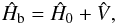 (1)where
Ĥ0 represents all the electronic and vibrational terms, and
(1)where
Ĥ0 represents all the electronic and vibrational terms, and
 is a perturbation operator. The subscript “b” indicates that, after taking account of all
interactions contained in Ĥb, the electronic states considered
occur in case b. The perturbation operator
is given by
is a perturbation operator. The subscript “b” indicates that, after taking account of all
interactions contained in Ĥb, the electronic states considered
occur in case b. The perturbation operator
is given by  (2)where
Ĥrot is the rotational Hamiltonian of the nuclei;
Ĥcd takes into account the centrifugal distortion of the
molecule; and Ĥso, Ĥsr, and
Ĥss arise respectively from the spin-orbital,
spin-rotational, and spin-spin interactions. We note that Ĥso
is zero for case b.
(2)where
Ĥrot is the rotational Hamiltonian of the nuclei;
Ĥcd takes into account the centrifugal distortion of the
molecule; and Ĥso, Ĥsr, and
Ĥss arise respectively from the spin-orbital,
spin-rotational, and spin-spin interactions. We note that Ĥso
is zero for case b.
Representing the total Hamiltonian Ĥb in the wave functions
in case a, | a ⟩, we have  (3)As a result of the
perturbation
(3)As a result of the
perturbation  ,
the Hamiltonian matrix ℋb becomes non-diagonal. However, the first term is
diagonal with respect to the electronic and vibrational state and gives the unperturbed
(and still degenerate) energy level E0. The second and the
third terms are the corrections to E0 of the first and of the
second order, respectively. The dots refer to the higher-order corrections to
E0. We considered here up to the third-order and forth-order
corrections arising from the spin-rotational and spin-spin interactions, respectively.
,
the Hamiltonian matrix ℋb becomes non-diagonal. However, the first term is
diagonal with respect to the electronic and vibrational state and gives the unperturbed
(and still degenerate) energy level E0. The second and the
third terms are the corrections to E0 of the first and of the
second order, respectively. The dots refer to the higher-order corrections to
E0. We considered here up to the third-order and forth-order
corrections arising from the spin-rotational and spin-spin interactions, respectively.
We diagonalize numerically the effective Hamiltonian (see, e.g., Brown & Carrington 2003) for the rotational levels of a
6Σ state that contains the -dependent
terms from the right-hand part of Eq. (3)
and that is given by Ram et al. (1993, Table 1). As
a result, we obtain the eigenvalues EΣJ, and
the eigenvectors of Ĥb in the absence of an external magnetic
field. The representation ⟨ b|Ĥb|b ⟩ in the wave functions
in case b is then diagonal with respect to the rotational state
| ΣJ ⟩.
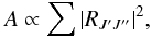
After the energy values EΣJ in both the upper A6Σ and the lower X6Σ electronic states have been obtained, one can calculate the energies of all possible electronic transitions in the (0,0) band allowed by the quantum mechanical selection rules. The line positions calculated are in a good agreement with those analyzed by Ram et al. (1993) and computed by Burrows et al. (2002).
2.2. Magnetic level structure
Now we consider the CrH molecule in the presence of an external magnetic field and examine its impact on the rotational structure calculated in Sect. 2.1.
When neglecting the interaction between the magnetic levels, the energy shift for a level
M at the magnetic field strength H, with respect to
its energy value in the absence of an external magnetic field, obtains as: 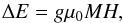 (4)where
g and μ0 are the Landé factor and the Bohr
magneton, respectively. The case, when the expression (4) holds, is called Zeeman regime (see, e.g., Berdyugina & Solanki 2002). However, as we show in Sect. 4.2, the ZR is practically not applicable for the CrH
6Σ electronic states (especially for the lower state), so the interaction
between magnetic levels cannot be neglected.
(4)where
g and μ0 are the Landé factor and the Bohr
magneton, respectively. The case, when the expression (4) holds, is called Zeeman regime (see, e.g., Berdyugina & Solanki 2002). However, as we show in Sect. 4.2, the ZR is practically not applicable for the CrH
6Σ electronic states (especially for the lower state), so the interaction
between magnetic levels cannot be neglected.
To take into account the interaction between the magnetic levels, i.e., to calculate the
Paschen-Back effect, we consider the total Hamiltonian of the molecule in the form
 (5)where the interaction of
the molecule with an external magnetic field
ĤH is considered to be smaller than the
intrinsic molecular interactions Ĥb. More precisely, we
consider here the case when ĤH is
significantly smaller than the sum
Ĥrot + Ĥcd, but it can be
comparable or larger than Ĥsr and
Ĥss. This implies that we do not take into account the
perturbation ĤH on the rotational structure,
and we consider its impact on the fine level structure only. We note that the values of
Ĥrot, Ĥcd,
Ĥsr, and Ĥss depend on the
angular momentum quantum numbers J and N, so the degree
of the level mixing for a given magnetic field strength varies within the fine structure
(here, it decreases for higher rotational levels). In other words, for two adjacent
rotational levels the mixing occurs at a certain magnetic field strength, which can be
deduced from measurements when the entire molecular band is modeled.
(5)where the interaction of
the molecule with an external magnetic field
ĤH is considered to be smaller than the
intrinsic molecular interactions Ĥb. More precisely, we
consider here the case when ĤH is
significantly smaller than the sum
Ĥrot + Ĥcd, but it can be
comparable or larger than Ĥsr and
Ĥss. This implies that we do not take into account the
perturbation ĤH on the rotational structure,
and we consider its impact on the fine level structure only. We note that the values of
Ĥrot, Ĥcd,
Ĥsr, and Ĥss depend on the
angular momentum quantum numbers J and N, so the degree
of the level mixing for a given magnetic field strength varies within the fine structure
(here, it decreases for higher rotational levels). In other words, for two adjacent
rotational levels the mixing occurs at a certain magnetic field strength, which can be
deduced from measurements when the entire molecular band is modeled.
To obtain the eigenvalues of Ĥmag, we proceed in the same way
as we did for the rotational level structure. Since Ĥb is
diagonal with respect to a rotational state | ΣJ ⟩, we express
Ĥmag in the eigenfunctions of
Ĥb, 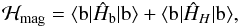 (6)where the second term is
non-diagonal with respect to the rotational state | ΣJ ⟩. We limit our
investigation of the molecular level structure to the first-order correction to the energy
value EΣJ, which is given by the second term
in the right-hand part of Eq. (6). Thus,
the Hamiltonian matrix ℋmag will be specified as
(6)where the second term is
non-diagonal with respect to the rotational state | ΣJ ⟩. We limit our
investigation of the molecular level structure to the first-order correction to the energy
value EΣJ, which is given by the second term
in the right-hand part of Eq. (6). Thus,
the Hamiltonian matrix ℋmag will be specified as
 (7)where the first
column and the first row refer to the eigenfunctions in case b. The
perturbation matrix has a trigonal form because, according to the first-order
approximation, only the perturbation of the adjacent levels within the multiplet structure
(fine structure) needs to be considered. Consequently, only the matrix elements forming
the main and secondary diagonals are distinct from zero. They are (Berdyugina et al. 2005, Table A.4)
(7)where the first
column and the first row refer to the eigenfunctions in case b. The
perturbation matrix has a trigonal form because, according to the first-order
approximation, only the perturbation of the adjacent levels within the multiplet structure
(fine structure) needs to be considered. Consequently, only the matrix elements forming
the main and secondary diagonals are distinct from zero. They are (Berdyugina et al. 2005, Table A.4)  where
the quantities μ0, M, H, and
S are, respectively, the Bohr magneton, the magnetic quantum number,
the magnetic field strength, and the total electron spin. The rotational quantum numbers
N and J obey the relation
N = J + Σ, where Σ is the projection of
S on the inter-nuclear axis. Each rotational level N
consists of six fine-structure levels, denoted by J
(J = N + 5/2, N + 3/2, ..., N−5/2),
owing to six possible projections of the total spin on the inter-nuclear axis. They are
degenerate in the absence of an external magnetic field, while in the presence of a
magnetic field each level J splits into 2J + 1 magnetic
levels M.
where
the quantities μ0, M, H, and
S are, respectively, the Bohr magneton, the magnetic quantum number,
the magnetic field strength, and the total electron spin. The rotational quantum numbers
N and J obey the relation
N = J + Σ, where Σ is the projection of
S on the inter-nuclear axis. Each rotational level N
consists of six fine-structure levels, denoted by J
(J = N + 5/2, N + 3/2, ..., N−5/2),
owing to six possible projections of the total spin on the inter-nuclear axis. They are
degenerate in the absence of an external magnetic field, while in the presence of a
magnetic field each level J splits into 2J + 1 magnetic
levels M.
By diagonalizing the Hamiltonian matrix (7) we obtain the eigenvalues EΣJM and the eigenvectors CΣJM of Ĥmag. In Sect. 3.2 we will make use of CΣJM to calculate the strengths of the magnetic transitions.
Figure 1 shows splitting of the fine structure levels of the upper and lower rotational levels N′ = 4 and N′′ = 3, respectively1, depending on the magnetic field strength. At a weak magnetic field (≲100 G for N′ = 4 and ≲10 G for N′′ = 3), the splitting is linear with the field strength and the interaction between the magnetic levels with the same quantum number M is negligible (ZR). As the field strength increases, the magnetic levels spread out and the levels with the same quantum number M repel each other. As a result, the magnetic levels form a blended structure in the PBR. Subsequently, at stronger magnetic fields (≳300 kG for N′ = 4 and ≳15 kG for N′′ = 3), the M levels are rearranged into a new multiplet structure corresponding to the six spin projections on the magnetic field direction (complete PBR).
Once the energy values EΣJM for both the upper A6Σ and the lower X6Σ electronic states have been obtained, magnetic transition energies can be calculated as their difference. Transition wavelengths are then obtained by correcting for the air refraction index according to Edlén (1966). We note that in addition to the main branch transitions (ΔJ = ΔN), we also consider here the satellite (ΔJ ≠ ΔN) and forbidden transitions as discussed by Berdyugina et al. (2005).
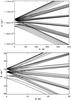 |
Fig. 1 Fine structure of the rotational levels N′ = 4 (top) and N′′ = 3 (bottom) in the presence of an external magnetic field. Each of the six fine structure levels J splits into 2J + 1 magnetic levels M, which are perturbed by nearby levels with the same M number. |
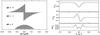 |
Fig. 2 Zeeman pattern and the corresponding Stokes profiles for the transition in Eq. (14) in the Zeeman regime. a) Zeeman pattern composed of three groups of lines that belong to the transitions with ΔM = 0, ± 1. The horizontal axis is dimensionless; it depicts the energy deviation, scaled by the factor μ0H, of the magnetic transitions with respect to the transition in the absence of a magnetic field. The height of the lines indicates the strength of the particular magnetic transition. The group of lines in the middle that belongs to the transitions with ΔM = −1 is plotted downwards for the sake of clarity. b) Stokes profiles I/Ic, V/Ic, and Q/Ic. The horizontal axis depicts the deviation in angstroms from the line center, which is set to 0. The vertical axis shows a strength of the particular Stokes signal and is different for each of the three panels. Again, the profiles here were obtained from the energy deviations scaled by the factor μ0H. |
3. Transition strengths
Intensity of a spectral line is proportional to the Einstein coefficient
A, which in turn is proportional to the sum of squares of the electric
dipole operator matrix elements
RJ′J′′,
 (8)where the sum is taken
over all levels contributing to the transition. Hence, our goal now is to compute the matrix
elements
RJ′J′′
in the PBR.
(8)where the sum is taken
over all levels contributing to the transition. Hence, our goal now is to compute the matrix
elements
RJ′J′′
in the PBR.
Following the discussion in Sect. 2, we first express the matrix elements RJ′J′′ in the case a basis functions, then transform them into case b to obtain the strengths of transitions in the ZR. Finally, we compute the strengths of transitions in the PBR using the eigenvectors of the magnetic Hamiltonian matrix (7).
3.1. ZR transition strengths
We employ the Born-Oppenheimer approximation to express the case a wave
functions | ΛSΣ; v; ΩJM ⟩ as a
product of the electronic | ΛSΣ ⟩, vibrational | v ⟩,
and rotational parts | ΩJM ⟩ (e.g., Schadee 1978):  (9)Correspondingly,
the right-hand part of Eq. (8) can be
expressed as a product of three numbers,
(9)Correspondingly,
the right-hand part of Eq. (8) can be
expressed as a product of three numbers, 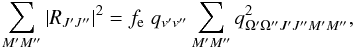 (10)where
fe is the electronic oscillator strength,
qv′v′′
is the Franck-Condon factor (both are constants for a given vibrational band), and
(10)where
fe is the electronic oscillator strength,
qv′v′′
is the Franck-Condon factor (both are constants for a given vibrational band), and
 is the
Hönl-London factor. The matrix elements
is the
Hönl-London factor. The matrix elements  and
qΩ′Ω′′J′J′′M′M′′
are called, respectively, strength and amplitude of a Zeeman component. It is the value of
this amplitude that distinguishes the ZR (in both cases, a and
b) from the PBR.
and
qΩ′Ω′′J′J′′M′M′′
are called, respectively, strength and amplitude of a Zeeman component. It is the value of
this amplitude that distinguishes the ZR (in both cases, a and
b) from the PBR.
In the ZR, the matrix elements
qΩ′Ω′′J′J′′M′M′′
can be further expressed as a product of two factors to separate the dependence on the
quantum number M:  (11)Expressions for
the amplitudes
qΩ′Ω′′J′J′′
and
qJ′J′′M′M′′
are given by Schadee (1978, Table I).
(11)Expressions for
the amplitudes
qΩ′Ω′′J′J′′
and
qJ′J′′M′M′′
are given by Schadee (1978, Table I).
Now we can obtain the matrix elements  represented
in the case b wave functions. First, for the
M-independent part of the transition amplitude we obtain
represented
in the case b wave functions. First, for the
M-independent part of the transition amplitude we obtain 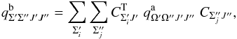 (12)where
CΣi,jJ are the
eigenvectors obtained by diagonalizing the Hamilton matrix (3), and
(12)where
CΣi,jJ are the
eigenvectors obtained by diagonalizing the Hamilton matrix (3), and  are
transposed vectors. Indices i and j relate to different
spin projections for the level with the total angular momentum quantum number
J; Σi and Σj
take values −5/2, −3/2, ...,
5/2. The second factor in Eq. (11),
qJ′J′′M′M′′,
is not affected by the transformation between the cases a and
b, and remains the same in both coupling cases. Hence, the total ZR
amplitude in the case b wave functions is
are
transposed vectors. Indices i and j relate to different
spin projections for the level with the total angular momentum quantum number
J; Σi and Σj
take values −5/2, −3/2, ...,
5/2. The second factor in Eq. (11),
qJ′J′′M′M′′,
is not affected by the transformation between the cases a and
b, and remains the same in both coupling cases. Hence, the total ZR
amplitude in the case b wave functions is  (13)By computing the
energies and the strengths of all magnetic transitions between two rotational states in
the presence of an external magnetic field we obtain a so-called Zeeman pattern. In the
ZR, it consists of three distinguished groups of lines which correspond to the transitions
with ΔM = 0, ± 1 and are called π-
and σ±-components. An example is shown in Fig. 2a, where a Zeeman pattern is calculated for the
transition
(13)By computing the
energies and the strengths of all magnetic transitions between two rotational states in
the presence of an external magnetic field we obtain a so-called Zeeman pattern. In the
ZR, it consists of three distinguished groups of lines which correspond to the transitions
with ΔM = 0, ± 1 and are called π-
and σ±-components. An example is shown in Fig. 2a, where a Zeeman pattern is calculated for the
transition  (14)in the
R spectroscopic branch assuming the ZR.
(14)in the
R spectroscopic branch assuming the ZR.
As Eq. (4) for the ZR predicts, the energy shifts are linear with the magnetic field strength. Therefore, the Zeeman pattern in Fig. 2a is symmetric. If the ZR holds for this line, its shape does not change with the magnetic field strength. However, this is not the case for the CrH lines under consideration, and we need to proceed with the following step to find an expression for the transition strengths in the PBR.
3.2. PBR transition strengths
The transformation of the amplitudes from the ZR in case b to the PBR is
carried out with the help of the eigenvectors
CΣi,jJM
obtained by diagonalizing the Hamiltonian matrix (7), 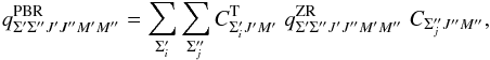 (15)where the indices
i and j again relate to the different levels
J that form a fine structure of a rotational level N;
Σi and Σj take values
−5/2, −3/2, ..., 5/2. In
contrast to the ZR amplitude (13), the PBR
amplitude (15) is no longer a product of
two factors, but a linear combination of the ZR transition amplitudes.
(15)where the indices
i and j again relate to the different levels
J that form a fine structure of a rotational level N;
Σi and Σj take values
−5/2, −3/2, ..., 5/2. In
contrast to the ZR amplitude (13), the PBR
amplitude (15) is no longer a product of
two factors, but a linear combination of the ZR transition amplitudes.
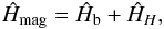
In Figs. 3a, 3c, 3e, 3g, and 3i we show the Zeeman patterns for the transition in Eq. (14) in the PBR for the magnetic field strengths 0.001, 0.01, 0.1, 1, and 10 kG, respectively. The Zeeman pattern in Fig. 3a appears quite symmetric; in other words, the upper and lower N levels of the molecule seem to be in the ZR at 0.001 kG. However, the corresponding Stokes Q/Ic profile (Fig. 3b) is clearly asymmetric (see our discussion in Sect. 4.2). As the magnetic field strength increases, the pattern evolves rapidly, because the energy shifts no longer vary linearly, as Eq. (4) predicts. At stronger magnetic fields the shape of the pattern changes dramatically (Figs. 3 e,g,i): the Zeeman shifts change their sign (the pattern appears twisted), and the Zeeman component strengths alter significantly. In this example of the R spectroscopic branch (ΔJ = 1), σ+ components become stronger than σ− and π components in a strong field regime (cf., Fig. 3g). This is in contrast to the P branch (ΔJ = −1), where σ− transitions become dominant (not shown). Thus, considering a great number of rotational transitions we expect a net polarization in the (0,0) band of the CrH molecule.
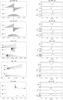 |
Fig. 3 Zeeman patterns and the corresponding Stokes profiles for the transition in Eq. (14) calculated for different magnetic field strengths. |
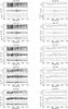 |
Fig. 4 Stokes profiles for the (0,0) band of the
A |
4. Radiative transfer calculations
The theoretical line parameters calculated as described in the previous sections have been used to synthesize the Stokes profiles for both individual lines and the entire (0,0) band with the code STOPRO (described by Solanki 1987; Frutiger et al. 1999; Berdyugina et al. 2003). The code assumes local thermodynamic equilibrium (LTE) and solves numerically a set of polarized transfer equations in a model atmosphere. Furthermore, it is assumed that a magnetized atmosphere acts on a spectral line (both atomic and molecular) through the Zeeman or Paschen-Back effect. The polarization arising from scattering in the atmosphere is neglected. Number densities of about 300 atomic and molecular species are calculated under the assumption of the chemical equilibrium as described in Berdyugina et al. (2003).
4.1. Atmosphere models and condensate opacities
We employ the original Drift-Phoenix atmospheric models calculated by Witte et al. (2009) for Teff = 2500 K, 2000 K, and 1500 K. The solar abundances of the chemical elements and the surface gravity of log g = 5.0 is assumed. These three atmospheric models correspond roughly to the physical parameters of late M dwarfs, early and mid-L dwarfs, and hot Jupiters.
In atmospheres of cool brown dwarfs and hot exoplanets dust can considerably contribute to the total opacity. The Drift-Phoenix models, for example in contrast to the Phoenix model grid by Allard & Hauschildt (1995), employ the physics of dust formation and predict abundances of such condensate species as TiO2, Al2O3, Fe, SiO2, MgO, MgSiO3, and Mg2SiO4. Since their significance as opacity sources increases for lower temperature and higher pressure, we want to estimate the effect of dust scattering and absorption on the CrH spectrum in the three selected models. To do this, we make use of an analytical solution of the Mie theory (Mie 1908).
The opacity ϰ caused by the interaction of the radiation with dust particles is related
to the interaction cross section σ in the relation  (16)where
σ = σsca + σabs
is the sum of the cross sections due to scattering and absorption of the radiation, and
N is the number of the dust particles within a unit volume.
(16)where
σ = σsca + σabs
is the sum of the cross sections due to scattering and absorption of the radiation, and
N is the number of the dust particles within a unit volume.
To calculate the interaction cross section σ, we employ an analytical
expression obtained for scattering and absorption of electromagnetic waves by small
(compared with the radiation wavelength) spherical particles (see, e.g., Landau & Lifshitz 1960),  (17)where a
is the particle size (radius), λ is the wavelength of the incident
electromagnetic wave; ε and ε′′ are the
relative dielectric function and its imaginary part of the particle material.
(17)where a
is the particle size (radius), λ is the wavelength of the incident
electromagnetic wave; ε and ε′′ are the
relative dielectric function and its imaginary part of the particle material.
The Drift-Phoenix model grid provides the following depth-dependent dust parameters: average grain size, number of particles in the unit volume, and volume fraction for each dust species. Since we have the average particle size rather than the individual particle sizes of each species, we calculate the corresponding average (volume-fraction-weighted) relative dielectric function according to the effective medium theory (see, e.g., Bohren & Huffman 1998). Thus, Eq. (17) was evaluated using the average grain size and the average relative dielectric function.
We have found that for the chosen model atmospheres the opacity due to light scattering on the dust particles is significantly larger than light absorption by these particles at the CrH band wavelength. Furthermore, the total condensate opacity in Eq. (16) becomes considerable (at a level of a few percent) with the gas opacity only for the Teff = 1500 K model and, respectively, for cooler atmospheres. We note that this condensate opacity contribution is already included in the atmospheric models used.
4.2. Stokes profiles
First we calculate the Stokes profiles for the individual lines at the magnetic field strengths 0.001, 0.01, 0.1, 1, and 10 kG. As an example, the inclination of the magnetic field γ is set to 45° and the azimuth χ to 0° in all calculations presented in this paper. Hence, both Stokes V and Q are distinct from zero, while the Stokes U vanishes. We normalize the Stokes parameters to the continuum intensity Ic.
Figures 2 and 3 show the Stokes profiles for the transition in Eq. (14) assuming the ZR and PBR, respectively. A remarkable feature in Figs. 3b, 3d, 3f, 3h, and 3j is that neither of the Stokes Q/Ic shows a symmetric shape as it does in Fig. 2b. This originates because the states contributing to the transition (at least one of them) are in the PBR. Even at a weak magnetic field (about 0.001 kG) the ZR is inappropriate for many lines from the (0,0) band, as revealed by the non-symmetric Stokes Q/Ic (Fig. 3b). Indeed, the deviation of the magnetic levels from their degenerate position depends linearly on the magnetic field strength as long as the sub-levels with the same magnetic quantum number do not come close to each other. Otherwise, the sub-levels with the same number M begin to interact (repel), so that the linear dependence from the magnetic field strength, demonstrated by Eq. (4), is no longer guaranteed. Because the separation of the fine structure levels that split in the presence of a magnetic field is not equidistant, and some levels can lie very close together, as shown in Fig. 1, the ZR fails for such levels even at very small magnetic field strengths. Our careful investigation shows that the Stokes Q/Ic is especially sensitive to the shifts of the magnetic transitions with respect to their frequency in the absence of an external magnetic field. In other words, even tiny deviations from Eq. (4) cause a non-symmetric Stokes Q/Ic.
Figures 4–6 show the Stokes profiles calculated for the entire (0,0) band for Teff = 2500 K, 2000 K, and 1500 K, respectively, in the wavelength range 8600−8700 Å at the magnetic field strengths 0.5, 1, 3, 6, and 10 kG. The line list used includes about 500 CrH lines calculated using the theory given in Sect. 2. Very weak forbidden and satellite lines were sorted out from the list. Natural and pressure induced line broadening were included in the calculations. In addition, effects of low spectral resolution and possible fast stellar rotation were taken into account.
We have found that the Stokes V/Ic spectra show significant signals at the field strengths considered. In general, polarization signals increase for stronger magnetic fields from a few percent at 0.5 kG to more than 20% at fields of several kG when observed at high spectral resolution. In addition, the polarization signal arising from some lines or groups of lines (e.g., near 8625 or 8685 Å) shows a considerable asymmetry due to the Paschen-Back effect in these lines (cf. panels a and b in Figs. 4−6). Furthermore, the satellite lines (ΔJ ≠ ΔN) gain in strength, while the main lines (ΔJ = ΔN) become weaker (cf. Stokes I/Ic in Figs. 4a, 4c, 4e, 4g, 4i). Thus, the polarization signal coming from a great number of satellite lines becomes comparable with that coming from the main lines. It reaches 25% in Stokes V/Ic and 15% in Stokes Q/Ic at 10 kG (cf. Figs. 4a, 4c, 4e, 4g, 4i). Moreover, while the magnetic field strength increases, the absorption intensity (Stokes I/Ic) decreases noticeably. This is caused by redistribution of the radiative energy between main and satellite lines.
In the strong field regime, the Stokes V/Ic undergoes a crucial alteration: it becomes asymmetric over a wide range of wavelengths (cf. panels f, h, and j in Figs. 4–6) leading to a large scale broad-band polarization, which can be detected even at a much lower spectral resolution. For instance, magnetic fields of 6 kG and stronger could be detected on very faint brown dwarfs using this feature.
5. Conclusions
We have explored the magnetic sensitivity of the (0,0) vibrational band
from the A–
X system of
the CrH molecule and developed a new diagnostic for magnetic field measurements on very cool
stars, brown dwarfs, and, potentially, on hot Jupiters.
Our quantum mechanical calculations of the energy level structure of the CrH (0,0) band in the absence of an external magnetic field reproduce well the results of Ram et al. (1993) and are in a good agreement with the results obtained by Kleman & Uhler (1959) and Burrows et al. (2002).
Employing the approach by Berdyugina et al. (2005) for predicting the magnetic level structure of electronic states of any multiplicity in diatomic molecules, we have calculated for the first time the CrH level structure in the presence of an external magnetic field. Transition frequencies and their strengths are obtained in both the ZR and PBR.
We confirm the following general behavior of transition strengths in the PBR as the magnetic field strength increases (Berdyugina et al. 2005). First, satellite lines become stronger, while the main branch lines weaken. In addition, σ+ components (ΔM = 1) become stronger than σ− components (ΔM = −1) in the R branch, while the opposite is true for the P branch.
Our detailed study of a number of Stokes profiles of the individual CrH lines shows that even at weak magnetic fields (~1 G) Eq. (4) for the energy shifts in the ZR becomes inadequate for many of these lines. In general, the energy shifts due to an external magnetic field must be considered non-linear at any magnetic field strength, even though the deviations from the ZR are approaching zero at a very weak magnetic field.
A spectral synthesis of the CrH (0,0) band at different magnetic field strengths (0.5−10 kG) has revealed the following general behavior of the spectra as the field strength increases:
-
the band profile varies with the magnetic field strength;
-
absorption in Stokes I/Ic decreases;
-
polarization, particularly Stokes V/Ic, increases;
-
Stokes profiles become asymmetric;
-
integral polarization over the band is distinct from zero (broad-band polarization).
objects. Based on our results, fields of ~100 G and stronger can be detected with existing instruments. This lower limit has two origins: i) at weaker magnetic fields the polarization degree is too small to be detected, and ii) most of lines in the band are not yet in the complete PBR to produce a considerable asymmetry in the Stokes V/Ic signal.
The calculations presented do not include a filling factor for magnetic regions on the stellar surface because it is not well known for brown dwarfs; however, its effect is linear. Taking into account a filling factor, which is a positive rational number between 0 and 1, will proportionally reduce the intensity of a polarization signal. However, this does not affect the asymmetry and the shape of the signal. Therefore, an analysis of the line (or band) profiles in the PBR can provide unambiguous estimates of both the magnetic field strength and its filling factor. This is in contrast to the ZR, when only a product of these two quantities can be inferred.
The wavelength range considered (8600−8700 Å) includes blends other than CrH lines (e.g., FeH and TiO lines). These have to be taken into account when evaluating and interpreting the observational data.
Overall, we conclude that the CrH A –
X system is
a very sensitive magnetic diagnostic for cool substellar objects, and we will employ it for
our studies of brown dwarfs in the near future.
Throughout this paper, we use single and double primes to indicate upper and lower levels, respectively.
Acknowledgments
We are grateful to P. Bernath for his helpful advice on the calculation of the rotational structure of the CrH. We thank Ch. Helling and S. Witte for providing us with the Drift-Phoenix model atmospheres and the corresponding dust properties. This work was supported by the grant of the Leibniz Association SAW-2011-KIS-7, ERC Advanced Grant HotMol, and the NASA Astrobiology Institute.
References
- Afram, N., Berdyugina, S., Fluri, D., et al. 2008, A&A, 482, 387 [NASA ADS] [CrossRef] [EDP Sciences] [Google Scholar]
- Allard, F., & Hauschildt, P. 1995, ApJ, 445, 433 [NASA ADS] [CrossRef] [Google Scholar]
- Berdyugina, S. V. 2011, ASPC, 437, 219 [Google Scholar]
- Berdyugina, S. V., & Solanki, S. 2002, A&A, 385, 701 [NASA ADS] [CrossRef] [EDP Sciences] [Google Scholar]
- Berdyugina, S. V., Solanki, S., & Frutiger, C. 2003, A&A, 412, 513 [NASA ADS] [CrossRef] [EDP Sciences] [Google Scholar]
- Berdyugina, S. V., Braun, P., & Fluri, D. 2005, A&A, 444, 947 [NASA ADS] [CrossRef] [EDP Sciences] [Google Scholar]
- Berdyugina, S. V., Berdyugin, A. V., & Piriiola, V. 2007, Phys. Rev. Lett., 99, 1 [Google Scholar]
- Bernath, P. 2009, Int. Rev. Phys. Chem., 28, 681 [CrossRef] [Google Scholar]
- Bohren, C., & Huffman, D. 1998, Absorption and Scattering of Light by Small Particles (John Wiley & Sons) [Google Scholar]
- Brown, J., & Carrington, A. 2003, Rotational Spectroscopy of Diatomic Molecules (Cambridge University Press) [Google Scholar]
- Burrows, A., Ram, R. S., Bernath, P., et al. 2002, ApJ, 577, 986 [NASA ADS] [CrossRef] [Google Scholar]
- Edlén, B. 1966, Metrologia, 2, 71 [NASA ADS] [CrossRef] [Google Scholar]
- Engvold, O., Wöhl, H., & Brault, J. W. 1980, A&AS, 42, 209 [NASA ADS] [Google Scholar]
- Frutiger, C., Solanki, S., Fligge, M., et al. 1999, Solar polarization (Boston, Mass: Kluwer Academic Publishers), 281 [Google Scholar]
- Kirkpatrick, J., Reid, I., Liebert, J., et al. 1999, ApJ, 519, 802 [NASA ADS] [CrossRef] [Google Scholar]
- Kleman, B., & Uhler, U. 1959, Canad. J. Phys., 37, 537 [NASA ADS] [CrossRef] [Google Scholar]
- Landau, L., & Lifshitz, E. 1960, Course of Theoretical Physics, Electrodynamics Of Continuous Media (Pergamon Press), 8 [Google Scholar]
- Mie, G. 1908, Ann. Phys., 330, 377 [Google Scholar]
- Nakajima, T., Oppenheimer, B., Kulkarni, S., et al. 1995, Nature, 378, 463 [NASA ADS] [CrossRef] [Google Scholar]
- Pavlenko, Y. 1999, Astron. Rep., 43, 748 [NASA ADS] [Google Scholar]
- Ram, R., Jarman, C., & Bernath, P. 1993, J. Mol. Spectr., 161, 445 [NASA ADS] [CrossRef] [Google Scholar]
- Schadee, A. 1978, J. Quant. Spectr. Rad. Transf., 19, 517 [Google Scholar]
- Shulyak, D., Reiners, A., Wende, S., et al. 2010, A&A, 523, A37 [NASA ADS] [CrossRef] [EDP Sciences] [Google Scholar]
- Solanki, S. 1987, Ph.D. Thesis, ETH Zuerich [Google Scholar]
- Sriramachandran, P., & Shanmugavel, R. 2011, Ap&SS, 336, 379 [NASA ADS] [CrossRef] [Google Scholar]
- Witte, S., Helling, C., & Hauschildt, P. 2009, A&A, 506, 1367 [NASA ADS] [CrossRef] [EDP Sciences] [Google Scholar]
All Figures
|
Fig. 1 Fine structure of the rotational levels N′ = 4 (top) and N′′ = 3 (bottom) in the presence of an external magnetic field. Each of the six fine structure levels J splits into 2J + 1 magnetic levels M, which are perturbed by nearby levels with the same M number. |
| In the text | |
|
Fig. 2 Zeeman pattern and the corresponding Stokes profiles for the transition in Eq. (14) in the Zeeman regime. a) Zeeman pattern composed of three groups of lines that belong to the transitions with ΔM = 0, ± 1. The horizontal axis is dimensionless; it depicts the energy deviation, scaled by the factor μ0H, of the magnetic transitions with respect to the transition in the absence of a magnetic field. The height of the lines indicates the strength of the particular magnetic transition. The group of lines in the middle that belongs to the transitions with ΔM = −1 is plotted downwards for the sake of clarity. b) Stokes profiles I/Ic, V/Ic, and Q/Ic. The horizontal axis depicts the deviation in angstroms from the line center, which is set to 0. The vertical axis shows a strength of the particular Stokes signal and is different for each of the three panels. Again, the profiles here were obtained from the energy deviations scaled by the factor μ0H. |
| In the text | |
|
Fig. 3 Zeeman patterns and the corresponding Stokes profiles for the transition in Eq. (14) calculated for different magnetic field strengths. |
| In the text | |
|
Fig. 4 Stokes profiles for the (0,0) band of the
A |
| In the text | |
 |
Fig. 5 Same as Fig. 4, but for Teff = 2000 K. |
| In the text | |
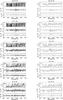 |
Fig. 6 Same as Fig. 4, but for Teff = 1500 K. |
| In the text | |
Current usage metrics show cumulative count of Article Views (full-text article views including HTML views, PDF and ePub downloads, according to the available data) and Abstracts Views on Vision4Press platform.
Data correspond to usage on the plateform after 2015. The current usage metrics is available 48-96 hours after online publication and is updated daily on week days.
Initial download of the metrics may take a while.