| Issue |
A&A
Volume 557, September 2013
|
|
|---|---|---|
| Article Number | A49 | |
| Number of page(s) | 12 | |
| Section | Celestial mechanics and astrometry | |
| DOI | https://doi.org/10.1051/0004-6361/201321843 | |
| Published online | 28 August 2013 | |
New analytical planetary theories VSOP2013 and TOP2013⋆
1
IMCCE, Observatoire de Paris, UMR CNRS 8028,
UPMC,
75014
Paris,
France
e-mail:
This email address is being protected from spambots. You need JavaScript enabled to view it.
2
SYRTE, Observatoire de Paris, UMR CNRS 8630,
UPMC,
75014
Paris,
France
e-mail:
This email address is being protected from spambots. You need JavaScript enabled to view it.
3
GéoAzur, Observatoire de la Côte d’Azur, UNR CNRS 7329,
04870 Côte
d’Azur,
France
e-mail:
This email address is being protected from spambots. You need JavaScript enabled to view it.
Received:
6
May
2013
Accepted:
19
June
2013
Abstract
Context. The development of precise numerical integrations of the motion of the planets, taking into account the most recent observations, lead us to improve the two families of analytical planetary theories built in the Institut de mécanique céleste et de calcul des éphémérides (IMCCE), the Variations Séculaires des Orbites Planétaires (VSOP) and the Theory of the Outer Planets (TOP) theories.
Aims. We have built the solutions VSOP2010 and TOP2010 fitted to the Jet Propulsion Laboratory (JPL) numerical integration DE405 and the solutions VSOP2013 and TOP2013 fitted to the European recent numerical integration INPOP10a. This paper specifically considers VSOP2013 and TOP2013.
Methods. We have improved the construction of VSOP by analytically computing the pertubations due to the asteroids and to Pluto. We have increased the precision of the VSOP solutions of Jupiter and Saturn by using TOP solutions. We have also improved the construction of TOP by computing the perturbations due to the telluric planets from VSOP solutions. Moreover, TOP contains a solution of the motion of the Pluto-Charon barycenter.
Results. From 1890 to 2000, the precision of VSOP2013 goes from a few 0.01 mas (planets except Mars and Uranus) up to 0.7 mas (Mars and Uranus). Compared to the previous solution (VSOP2000), this represents an improvement of a factor of 2 to 24, depending on the planet. From −4000 to 8000, the precision is of a few 0.1″ for the telluric planets (1.6″ for Mars), i.e. an improvement of about a factor of 5 compared to VSOP2000. The TOP2013 solution is the best for the motion of the major planets from −4000 to 8000. Its precision is of a few 0.1″ for the four planets, i.e. a gain between 1.5 and 15, depending on the planet compared to VSOP2013. The precision of the theory of Pluto remains valid up to the time span from 0 to 4000. The VSOP2013 and TOP2013 data are available on the WEB server of the IMCCE.
Key words: celestial mechanics / ephemerides
VSOP2013 and TOP2013 are available by ftp on: ftp.imcce.fr/pub/ephem/planets/vsop2013 and ftp.imcce.fr/pub/ephem/planets/top2013.
© ESO, 2013
1. Introduction
For the last 30 years, two kinds of analytical planetary theories1 have been built in the Institut de mécanique céleste et de calcul des éphémérides (IMCCE): the Variations Séculaires des Orbites Planétaires (VSOP) theories, essentially issued from the research works of P. Bretagnon, and the Theory of Outer Planets (TOP) theories, derived from the works of J.-L. Simon. The VSOP theories are solutions for the motion of the eight planets in the solar system; they are very precise over a time span of about 1000 years and the ephemerides published by the IMCCE from 1984 to 2006 were derived from VSOP. The TOP theories are solutions for the motion of the four major planets and are accurate over several thousands of years. Currently, the ephemerides of the planets are obtained mainly from very precise numerical integrations fitted to the most recent observations: the European ephemerides Intégration Numérique Planétaire de l’Observatoire de Paris (INPOP, Fienga et al. 2008, 2009, 2011), the American ephemerides Development Ephemeris (DE; e.g. Standish 1998; or more recently Folkner et al. 2009; Folkner 2010) and the Russian ephemerides Ephemerides of Planets and the Moon (EPM; Pitjeva 2005, 2010). Nevertheless, the construction of analytical planetary theories remains useful: (i) even if the aim of analytical theories is not to compete with numerical integrations for space engineering, they can provide precise ephemerides for the concern of most astronomers; (ii) their precision slowly decrease with time and they remain accurate over several thousand years; (iii) they allow a precise analysis of the perturbations; (iv) they are useful for some problems such as the study of the Earth’s rotation; and (v) from these theories it is possible to obtain compact solutions of good precision.
We first built the analytical solutions VSOP2010 and TOP2010, fitted to DE405 (Standish 1998). We then built VSOP2013 and TOP2013, fitted to INPOP10a (Fienga et al. 2011). This paper particularly deals with VSOP2013 and TOP2013. After giving the common characteristics of these two kinds of solutions in Sect. 2, we will present the construction of the VSOP theories (Sect. 3) and of the TOP theories (Sect. 4). A method to build an analytical solution of the motion of Pluto is given in Sect. 5. Perturbations by asteroids are studied in Sect. 6. Lastly, the results are presented and discussed in Sect. 7.
2. Common characteristics
The two solutions VSOP and TOP have several characteristics in common that are given here.
2.1. Variables and equations
-
The variables used are the elliptic variables a, λ, k = ecosϖ, h = esinϖ, q = sini/2cosΩ, and p = sini/2sinΩ where a is the semi-major axis, λ the mean longitude, e the eccentricity of the orbit, ϖ the longitude of perihelion, i the inclination to the ecliptic J2000, and Ω the longitude of the ascending node.
-
The equations of the motion of the planets are the Lagrange differential equations (for the computing of the second members of the Lagrange equations, see Chapront et al. 1975).
2.2. Form of the solutions
There are two kinds of analytical planetary theories: general planetary theories and
classical planetary theories. In general planetary theories, the variables are developed
under the form of Fourier series, with arguments being linear combinations of short-period
arguments (mean longitudes of the planets) and long-period arguments (longitudes of nodes
and perihelia). Developing the long-period arguments with respect to time, we obtain the
classical planetary theories under the form of Poisson series, with arguments being linear
combinations of short-period arguments. The VSOP and TOP solutions are classical planetary
theories. For a planet j, we note that
xj are the elements other than mean
longitudes λj;
xj and
λj have the form
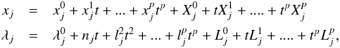 (1)where
t is the time (the timescale will be explained in the following
sections),
(1)where
t is the time (the timescale will be explained in the following
sections),  and
and
 are numerical
coefficients, and
are numerical
coefficients, and  and
and
 are Fourier
series of short-period arguments the form of which will be explained in the following
sections.
are Fourier
series of short-period arguments the form of which will be explained in the following
sections.
2.3. Integration of the equations
-
Results of the integration are obtained in the following way. First, the perturbations are built order by order up to the third order with respect to the masses. An iterative method is then used for the following computations.
-
The integration constants
 and
and
 and the
mean motions nj are determinated by
fitting, over the time span from 1890 to 2000, the solutions to the numerical
integrations DE405 (Standish 1998) for the
solutions VSOP2010 and TOP2010 or INPOP10a (Fienga
et al. 2011) for VSOP2013 and TOP2013. We note that the numerical formulae
given in the following sections will generally relate to the solutions fitted to
INPOP10a.
and the
mean motions nj are determinated by
fitting, over the time span from 1890 to 2000, the solutions to the numerical
integrations DE405 (Standish 1998) for the
solutions VSOP2010 and TOP2010 or INPOP10a (Fienga
et al. 2011) for VSOP2013 and TOP2013. We note that the numerical formulae
given in the following sections will generally relate to the solutions fitted to
INPOP10a.
3. The VSOP theories
The VSOP theories are analytical theories for the eight planets: Mercury, Venus, the Earth-Moon barycenter (EMB), Mars, Jupiter, Saturn, Uranus, and Neptune.
3.1. Historical review
The first VSOP solutions were:
-
VSOP82 (Bretagnon 1982). In this solution, the iterative method was developed up to the fifth order with respect to the masses. The relativity was introduced by the Schwarzschild problem and the perturbations of the Earth-Moon barycenter by the Moon were taken into account. So, the arguments of the Poisson series were the mean mean longitudes of the planets and the Delaunay arguments of the Moon D, F, and L. The mean mean longitudes are linear functions of time defined for each planet j by
 (2)where
nj is the mean motion of the planet
j. VSOP82 was fitted to the numerical integration of the JPL,
DE200 (Standish 1982). The timescale is
barycentric dynamical time (TDB) obtained from Fairhead & Bretagnon (1990).
(2)where
nj is the mean motion of the planet
j. VSOP82 was fitted to the numerical integration of the JPL,
DE200 (Standish 1982). The timescale is
barycentric dynamical time (TDB) obtained from Fairhead & Bretagnon (1990). -
VSOP87 (Bretagnon & Francou 1988). This solution was an extension of VSOP82, so this solution was also fitted to DE200. The solutions were expressed with elliptic elements and also with rectangular (X, Y, Z) or spherical (longitude, latitude, and radius vector) variables. The reference frames were the ecliptic and equinox J2000 or the ecliptic and equinox of the date. The coordinates were heliocentric or barycentric. VSOP82 and VSOP87 were used to compute the ephemerides of the IMCCE up to the construction of the INPOP numerical integrations (Fienga et al. 2009, 2011).
-
VSOP2000 (Moisson & Bretagnon 2001). This solution was an improvement of VSOP82. The iterative method was developed up to the eighth order of the masses. The perturbations by the five big asteroids Ceres, Pallas, Vesta, Iris, and Bamberga were introduced during the iterations. Second order perturbations by the Moon on Mercury, Venus, the Earth-Moon barycenter, and Mars were computed. Relativistic corrections were also introduced in the iterations. The arguments of the series were linear combinations of 16 angles, the mean mean longitudes of the eight major planets and of the five big asteroids, and the three Delaunay angles of the Moon. The solution was fitted to the numerical integration of the JPL DE403 (Standish et al. 1995). This solution was 10 to 100 times more precise than VSOP82 and VSOP87.
3.2. New VSOP theories
3.2.1. The works of P. Bretagnon
Starting in VSOP2000, Bretagnon performed 15 additional iterations with a numerical precision 10 times better than VSOP2000, with the following characteristics:
-
The Poisson series were developed up to the 12th degree with respect to time.
-
The eight major planets and the five big asteroids had their orbits analytically computed during the same process.
-
Perturbations of the Moon issued from ELP2000 (Chapront-Touze & Chapront 1983) on the eight major planets were introduced during the iteration process.
-
Relativistic corrections were introduced in the iterations.
-
The solution was fitted to DE403 (Standish et al. 1995) using the inertial mean ecliptic of J2000 defined by Chapront et al. (2002). Starting from the equatorial rectangular variables (x,y,z)equ given by DE403, we computed the ecliptic rectangular variables (x,y,z)ecl by
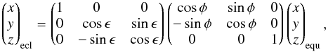 (3)where
ϵ and φ are issued from Chapront et al. (2002) as
(3)where
ϵ and φ are issued from Chapront et al. (2002) as
 (4)From
these ecliptic rectangular coordinates, we computed elliptic elements issued from
DE403 and we computed the integration constants by fitting elliptic elements of
VSOP to the elements issued from DE403 over the time span from 1890 to 2000. We
note that the inertial mean ecliptic J2000 that was used was very close to but not
exactly the same as the dynamic ecliptic of VSOP. So, the integration constants of
the variables q and p of the EMB were very small
but not equal to zero.
(4)From
these ecliptic rectangular coordinates, we computed elliptic elements issued from
DE403 and we computed the integration constants by fitting elliptic elements of
VSOP to the elements issued from DE403 over the time span from 1890 to 2000. We
note that the inertial mean ecliptic J2000 that was used was very close to but not
exactly the same as the dynamic ecliptic of VSOP. So, the integration constants of
the variables q and p of the EMB were very small
but not equal to zero.
3.2.2. The construction of the VSOP2010 and VSOP2013 solutions
Unfortunately, Bretagnon did not have time to complete his work. We took his work up again introducing various changes and supplements
-
The integration constants have been computed, first by fitting VSOP2010 to the numerical integration of the JPL DE405, then to different versions of the INPOP numerical integrations INPOP06 (Fienga et al. 2008), INPOP08 (Fienga et al. 2009), and finally INPOP10a (Fienga et al. 2011) for VSOP2013. These fits were done over the time span from 1890 to 2000.
-
We have computed the perturbations due to the J2 of the Sun on the planets Mercury, Venus, EMB, and Mars. The values used for the J2 of the Sun are 2 × 10⁻⁷ for DE405 and 2.4 × 10⁻⁷ for INPOP10a.
-
We have introduced the perturbations induced by the asteroids as explained in Sect. 6.
-
We have added the perturbations of Pluto on the outer planets in the form of Poisson series as explained in Sect. 5.4.5.
-
Starting from the TOP solutions, we have improved the precision of the theories of Jupiter and Saturn over a large time span as explained in Sect. 4.3.
-
The arguments of the series are linear combinations of 17 angles: the 16 angles of VSOP2000 and the linear function of time μ defined below.
-
The timescale is TDB and the relationship with terrestrial time (TT) depends on the ephemeris. For DE405, one can use TE405 (Irwin & Fukushima 1999). For INPOP10a, the transformation between TT and TDB is numerically integrated with the equations of the motion of the bodies, leading to a 4D-ephemeris (see Fienga et al. 2009).
-
The solutions are fitted with DE405 or INPOP10a as explained in Sect. 3.2.1. For the fit to DE405, we use the values given by Chapront et al. (2002)
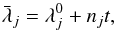
 (5)The fit
to INPOP10a is made starting from the equatorial rectangular coordinates of
INPOP10a and using the angles given in Eq. (5) to compute the ecliptic rectangular
coordinates, then the elliptic elements. The comparison, from 1890 to 2000, with
the elliptic elements issued from DE405 gives small corrections
Δq and Δp for p and
q of EMB. From these corrections, we deduce the corrections
Δϵ and Δφ by
(5)The fit
to INPOP10a is made starting from the equatorial rectangular coordinates of
INPOP10a and using the angles given in Eq. (5) to compute the ecliptic rectangular
coordinates, then the elliptic elements. The comparison, from 1890 to 2000, with
the elliptic elements issued from DE405 gives small corrections
Δq and Δp for p and
q of EMB. From these corrections, we deduce the corrections
Δϵ and Δφ by
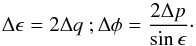 (6)We finally found
the values corresponding to INPOP10a:
(6)We finally found
the values corresponding to INPOP10a:
 (7)We note
that if, starting from the values in Eq. (5), we apply this method replacing
INPOP10a by DE403, we find
(7)We note
that if, starting from the values in Eq. (5), we apply this method replacing
INPOP10a by DE403, we find  and
φ = −0.05296″, values very close to the Chapront values
given in Eq. (4), that validates our method. The values found in Eq. (7) are
consistent with the ICRF (International Celestial Reference Frame) definition.
Indeed, by the fit of INPOP10a to planet positions obtained by VLBI (Very Long
Baseline Interferometry) tracking of spacecraft, INPOP10a is directly tied to ICRF
at the precision of these observations, about a few mas (Fienga et al. 2011). In consequence, VSOP2013 being fitted to
INPOP10a can then be seen as linked to ICRF by means of INPOP10a.
and
φ = −0.05296″, values very close to the Chapront values
given in Eq. (4), that validates our method. The values found in Eq. (7) are
consistent with the ICRF (International Celestial Reference Frame) definition.
Indeed, by the fit of INPOP10a to planet positions obtained by VLBI (Very Long
Baseline Interferometry) tracking of spacecraft, INPOP10a is directly tied to ICRF
at the precision of these observations, about a few mas (Fienga et al. 2011). In consequence, VSOP2013 being fitted to
INPOP10a can then be seen as linked to ICRF by means of INPOP10a.
We use the systems of planetary masses of DE405 for VSOP2010 and of INPOP10a for VSOP2013. We note G the newtonian gravitational constant and M the mass of a celestial body. Table 1 gives the GM of the Sun, the planets, and the five big asteroids used for the construction of INPOP10a.
GM of the Sun, the planets, and the five big asteroids used for the construction of INPOP10a.
4. The TOP theories
The TOP (Theory of the Outer Planets) theories are analytical theories for the motion of the four large planets Jupiter, Saturn, Uranus, and Neptune.
4.1. Historical review
The first TOP solutions were:
-
TOP82 (Simon 1983). In this solution, the perturbations were Poisson series of the mean mean longitudes of the four large Planets. A supplementary input was brought to the theory for the couple Jupiter-Saturn by computing, with an iterative method and using harmonic analysis, the mutual perturbations Jupiter-Saturn up to the seventh order with respect to the masses. The relativity was introduced as in VSOP82. The solution also contained the perturbations of the four large planets by the telluric planets at the third order of masses from VSOP82. TOP82 was fitted to DE200.
-
An extension of TOP82: JASON84 (Jupiter And Saturn Orbits from Neolithic). JASON84 (Simon & Bretagnon 1984) was an extension of TOP82 where the mutual perturbations Jupiter-Saturn were computed up to the 20th order of masses. Before the construction of the new TOP solutions, JASON84 was the most precise theory of the motion of Jupiter and Saturn over the time span [J2000-6000, J2000+6000] and was used to build the tables for the motion of those planets in the book Planetary Programs and Tables from −4000 to +2800 (Bretagnon & Simon 1986).
4.2. New TOP theories
The aim of TOP is not to compete with VSOP over a short time span but to build very precise theories of the four large planets over several thousands of years. For that purpose we use a completely different representation.
4.2.1. The representation
The solutions are also Poisson series of the form of Eqs. (1), but
and
are Fourier
series of only one argument
μ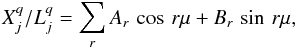 (8)where
r is a positive integer. The maximum value of r is
219(524 288) and μ is linked to the mean motions of
Jupiter and Saturn n5 and n6 by:
(8)where
r is a positive integer. The maximum value of r is
219(524 288) and μ is linked to the mean motions of
Jupiter and Saturn n5 and n6 by:
 (9)where
t is measured in thousands of years from J2000 and with the values of
n5 and n6 given in Table 6. The period of μ is about 17 485
years. The mean motions of the four major planets are linked to μ by
relations of the form
(9)where
t is measured in thousands of years from J2000 and with the values of
n5 and n6 given in Table 6. The period of μ is about 17 485
years. The mean motions of the four major planets are linked to μ by
relations of the form 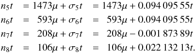 (10)This
representation was choosen because perturbations are more convergent using this form
than the classical form of Poisson series of the mean mean longitudes for Jupiter and
Saturn because the choice of μ allows us to take in account an
important part of the development with respect to the time of the long periods of a
general theory of the couple Jupiter-Saturn (Simon et
al. 1992). For Uranus and Neptune, the convergence is the same as in the
classical form.
(10)This
representation was choosen because perturbations are more convergent using this form
than the classical form of Poisson series of the mean mean longitudes for Jupiter and
Saturn because the choice of μ allows us to take in account an
important part of the development with respect to the time of the long periods of a
general theory of the couple Jupiter-Saturn (Simon et
al. 1992). For Uranus and Neptune, the convergence is the same as in the
classical form.
4.2.2. Construction of the solution
The solution is computed by the iterative method of Simon & Joutel (1988). The Lagrange equations are
 , with
F(μ,ti)
computed by harmonical analysis, for 13 values of the time
t0, t0 + Δt,
t0 − Δt, ...,
t0 + 6Δt,
t0 − 6Δt, t0
corresponding to J2000 and Δt = 1200 yrs. After interpolation and
integration, the solution has the form of Eqs. (1) with p = 12. The
integration constants have been computed by fitting TOP2010 to DE405 and TOP2013 to
INPOP10a, over the time span from 1890 to 2000.
, with
F(μ,ti)
computed by harmonical analysis, for 13 values of the time
t0, t0 + Δt,
t0 − Δt, ...,
t0 + 6Δt,
t0 − 6Δt, t0
corresponding to J2000 and Δt = 1200 yrs. After interpolation and
integration, the solution has the form of Eqs. (1) with p = 12. The
integration constants have been computed by fitting TOP2010 to DE405 and TOP2013 to
INPOP10a, over the time span from 1890 to 2000.
4.2.3. Perturbations by the telluric planets
For TOP2010, we used the perturbations by the telluric planets developed up to the third order of the masses extracted from VSOP82. They are written as μ series and are introduced in the iterations. For TOP2013, we obtain these perturbations by computing the differences between the last iteration of the iterative process used for VSOP2013 and the last iteration computed without taking in account the telluric planets. This method gives a better estimation of the perturbations by the telluric planets as will be seen in Sect. 7.3.2.
4.2.4. Heliocentric spherical and rectangular variables
It is easy to compute by harmonic analysis the heliocentric spherical variables (longitude, latitude, radius vector) and the heliocentric rectangular variables (X, Y, Z) from the elliptic elements, under the form of Poisson series of μ. These variables have been introduced in the TOP solutions.
Poisson developments of the mean longitude of Jupiter for the argument 4λ5 − 10λ6 for VSOP2013, TOP2013, TOP2013 in VSOP form, and corrections to VSOP2013.
4.3. Amelioration of VSOP theories using TOP theories
The good convergence of the mutual perturbations Jupiter-Saturn in the TOP solution can be used to improve the perturbations corresponding to some periodic terms in the VSOP representation of the semi-major axis and the mean longitude of these two planets. As an example of how the VSOP improvement is obtained for the Jupiter mean longitude development we take the argument 4λ5 − 10λ6.
4.3.1. VSOP and TOP developments
In VSOP, this development has the form
![Mathematical equation: \begin{equation} L_{v} = \sum_{p\,=\,0,11}t^p[ s_{4-10}^p \sin(4\lambda_5-10\lambda_6) + c_{4-10}^p\cos(4\lambda_5-10\lambda_6)]. \end{equation}](/articles/aa/full_html/2013/09/aa21843-13/aa21843-13-eq110.png) (11)This argument
corresponds to the TOP argument 38μ. The TOP development has the form
(11)This argument
corresponds to the TOP argument 38μ. The TOP development has the form
![Mathematical equation: \begin{equation} L_{t} = \sum_{q\,=\,0,12}t^q[ s_{38}^q \sin(38\mu) + c_{38}^q \cos(38\mu)]. \end{equation}](/articles/aa/full_html/2013/09/aa21843-13/aa21843-13-eq112.png) (12)The values of
(12)The values of
 and
and
 are given in
Cols. 2 and 3 of Table 2, and the values of
are given in
Cols. 2 and 3 of Table 2, and the values of
 and
and
 in Cols. 4
and 5. In Table 2, to estimate the amplitude of
the Poisson terms for t = ± 6000 yrs, the coefficients are given in
arcseconds for the periodic terms and in arseconds per 6000 years for the Poisson terms.
in Cols. 4
and 5. In Table 2, to estimate the amplitude of
the Poisson terms for t = ± 6000 yrs, the coefficients are given in
arcseconds for the periodic terms and in arseconds per 6000 years for the Poisson terms.
4.3.2. TOP developed in VSOP form
From Eqs. (10), we find  (13)where
t is measured in thousands of years from J2000. Substituting the
value of 38μ given by Eq. (13) in Eq. (12), we obtain a Poisson
development issued from TOP but under the VSOP representation. Up to
t20
(13)where
t is measured in thousands of years from J2000. Substituting the
value of 38μ given by Eq. (13) in Eq. (12), we obtain a Poisson
development issued from TOP but under the VSOP representation. Up to
t20
this development has the form ![Mathematical equation: \begin{equation} L_{tv} = \sum_{r\,=\,0,20}t^r[ s_{4-10}^{\prime r}\sin(4\lambda_5-10\lambda_6) + c_{4-10}^{\prime r}\cos(4\lambda_5-10\lambda_6)]; \end{equation}](/articles/aa/full_html/2013/09/aa21843-13/aa21843-13-eq116.png) (14)the values of
(14)the values of
 and
and  are given in Cols. 6 and 7 of Table 2.
4.3.3. Comparison between these developments
The comparison between the coefficients of the Cols. 2 and 3 of Table 2 with the coefficients of the Cols. 4 and 5 shows
the best convergence of the TOP representation. For instance, for
t = ± 6000 yrs the amplitude of the Poisson terms in
t9 is about 58″, 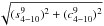 ,
for VSOP2013 and only 0.04″,
,
for VSOP2013 and only 0.04″,  ,
for TOP2013. The comparison between the coefficients of the Cols. 2 and 3 with the
coefficients of the Cols. 6 and 7 shows the inaccuracy of the VSOP representation from
Poisson terms in t11.
,
for TOP2013. The comparison between the coefficients of the Cols. 2 and 3 with the
coefficients of the Cols. 6 and 7 shows the inaccuracy of the VSOP representation from
Poisson terms in t11.
4.3.4. Correction of the VSOP development
The VSOP and TOP theories have been built in different ways and their integration
constants are not the same. So, the change of all VSOP coefficients of Eq. (11) by the
coefficients of Eq. (13) does not give good results. After some tests, we have estimated
that the best correction for this argument is to add to the VSOP coefficients the
differences between the coefficients of Eq. (13) and the coefficients of Eq. (11)
starting from Poisson terms in t9. So, these corrections
have the form ![Mathematical equation: \begin{equation} \delta L_{v} = \sum_{r\,=\,9,20}t^r[ \delta s_{4-10}^r \sin(4\lambda_5-10\lambda_6) + \delta c_{4-10}^r \cos(4\lambda_5-10\lambda_6)]. \end{equation}](/articles/aa/full_html/2013/09/aa21843-13/aa21843-13-eq123.png) (15)The values of
(15)The values of
 and
and
 are given in
Cols. 8 and 9 of Table 2.
are given in
Cols. 8 and 9 of Table 2.
4.3.5. Application of the method
This method has been applied to the Poisson developments of the semi-major axis and the mean longitude of Jupiter and Saturn for the 12 arguments
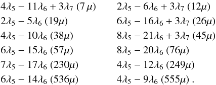 (16)Though
not rigorous, this method significantly improves the precision of VSOP for large time
spans, as we shall see in Sect. 7.4.2.
(16)Though
not rigorous, this method significantly improves the precision of VSOP for large time
spans, as we shall see in Sect. 7.4.2.
4.3.6. Degree of the Poisson development in VSOP
With these complements, the Poisson series of VSOP2013 and VSOP2010 are developed up to the 20th degree with respect to time.
5. Theory of the motion of Pluto
5.1. Perturbations by Pluto on the major planets
To obtain a precise theory of the major planets, especially for Uranus and Neptune, it is necessary to include the perturbations due to Pluto (or, more exactly, of the Pluto-Charon barycenter) and, therefore, to build an analytical theory of Pluto at least at the first order of masses.
5.2. Construction of the theory of Pluto in the classical form
A very close Neptune-Pluto resonance is the argument
 with a period of about 20 000 years,
  and
and  being the mean mean longitudes of Neptune and Pluto, respectively. Looking at Table 3, we can understand why the construction of a theory
of Pluto in the classical form is a complex problem. This table gives a few terms of the
perturbations at the first order with respect to the masses for the mean longitude,
computed with a precision of 5-11 rad (0.01 mas), for two couples of
planets:
being the mean mean longitudes of Neptune and Pluto, respectively. Looking at Table 3, we can understand why the construction of a theory
of Pluto in the classical form is a complex problem. This table gives a few terms of the
perturbations at the first order with respect to the masses for the mean longitude,
computed with a precision of 5-11 rad (0.01 mas), for two couples of
planets:
-
Saturn perturbed by Jupiter (which represents the most important first order perturbations obtained in the construction of an analytical theory of the eight planets),
-
Pluto perturbed by Neptune.
We can see that the amplitude of the most important perturbation of the mean longitude of
Pluto, 4.56 rad (9.4 × 10⁵ arcsec), which corresponds to the resonance
 ,
is greater than the most important perturbation of the mean longitude of Saturn, 0.013 rad
(2.7 × 10³ arcsec), by a factor of 350. Moreover, the number of terms greater
than 5-11 rad (0.01 mas) is 329 for Saturn perturbed by Jupiter and 15 539
for Pluto perturbed by Neptune. From the second iteration, the number of terms of the
perturbations of the mean longitude of Pluto soars and it becomes impossible to build an
analytical theory of Pluto in the classical form of series of the mean mean longitudes. In
our representation using μ, we obtain
,
is greater than the most important perturbation of the mean longitude of Saturn, 0.013 rad
(2.7 × 10³ arcsec), by a factor of 350. Moreover, the number of terms greater
than 5-11 rad (0.01 mas) is 329 for Saturn perturbed by Jupiter and 15 539
for Pluto perturbed by Neptune. From the second iteration, the number of terms of the
perturbations of the mean longitude of Pluto soars and it becomes impossible to build an
analytical theory of Pluto in the classical form of series of the mean mean longitudes. In
our representation using μ, we obtain
 (17)where the
coefficients of t are in rad/1000 yrs. The mean motion of Neptune
n8 is given in Table 6. For the mean motion of Pluto n9, we used a
preliminary value (25.350 505 rad/1000 yrs) given by Chapront (2012, priv. comm.). The
resonance
corresponds to the argument μ and we have exactly the same difficulties
as in the classical representation.
(17)where the
coefficients of t are in rad/1000 yrs. The mean motion of Neptune
n8 is given in Table 6. For the mean motion of Pluto n9, we used a
preliminary value (25.350 505 rad/1000 yrs) given by Chapront (2012, priv. comm.). The
resonance
corresponds to the argument μ and we have exactly the same difficulties
as in the classical representation.
5.3. Choice of a new argument for the representation
We chose a representation with an argument ν such that the resonance
should correspond to 0ν. So, the perturbations corresponding to the
resonance should be expanded in polynoms of time. We then take
 (18)where
t is measured in thousands of years from J2000 and with
n8 given in Table 6.
This argument is very near to μ given by Eq. (9) and we obtain
n9t = 70ν − 0.086 321 37t.
The resonance corresponds then to 0ν.
(18)where
t is measured in thousands of years from J2000 and with
n8 given in Table 6.
This argument is very near to μ given by Eq. (9) and we obtain
n9t = 70ν − 0.086 321 37t.
The resonance corresponds then to 0ν.
5.4. Construction of the analytical theory of Pluto
We built our theory of Pluto as explained in Simon (2004). As for the VSOP and TOP solutions, we built two solutions fitted to DE405 and INPOP10a, respectively.
5.4.1. First order theory
We first computed the mutual perturbations Jupiter-Pluto, Saturn-Pluto, Uranus-Pluto, and Neptune-Pluto in Poisson series of ν. The mutual perturbation Neptune-Pluto are computed without difficulties. For instance, the mean longitude of Pluto contains, for this couple, 44 terms with an amplitude greater than 0.01 mas (the amplitude of the most important term being about 30″) and 250 Poisson terms giving contributions greater than 0.01 mas over 1000 yrs. As an example, in the first order Saturn-Jupiter, computed in Poisson series of μ, the mean longitude of Saturn contains 329 terms with an amplitude greater than 0.01 mas and 496 Poisson terms giving contributions greater than 0.01 mas over 1000 yrs.
5.4.2. Construction of the theory
We applied the method used for building the TOP solutions for the combined and simultaneous resolution of two systems of equations in using the argument ν. The first system corresponds to the five planets Jupiter, Saturn, Uranus, Neptune, and Pluto, the second to the four major planets only. For the first iteration, we started from the first order theory for Pluto and from the TOP Poisson series of μ given in Poisson series of ν for the major planets. We also introduced the perturbations due to the telluric planets at the second order of masses. The resolution of the first system of equations gives the theory of the motion of Pluto. The differences between the solutions of the two systems give the perturbations of Pluto on the major planets.
5.4.3. The resonance 2 –3
–3 (0ν)
(0ν)
The secular terms corresponding to the resonance converge perfectly and decrease with time as can be seen in Table 4 which gives the values of the secular terms of the mean longitude of Pluto in ″/ 1000yrs.
Perturbations at the first order of the masses for the mean longitudes greater than 5 × 10-11 rad: comparison between Saturn perturbed by Jupiter and Pluto perturbed by Uranus.
Secular terms of the mean longitude of Pluto in ″/ 1000yrs.
Integration constants and mean motions of VSOP2013.
5.4.4. The argument  –
–
This argument has a period of 4000 yrs and corresponds to the argument
4ν like the great inequality Uranus-Neptune
 .
This argument is known as a long short-period argument, i.e. an argument with a period
similar to the periods of the long-period arguments of general theories. As shown by
Joutel (1990), in a classical planetary theory,
the perturbations corresponding to this type of argument do not converge well. Here, the
amplitude is about 700″ for the mean longitude of Pluto with an error of about 10″. We
shall discuss the consequences of this error in Sect. 7.3.2.
.
This argument is known as a long short-period argument, i.e. an argument with a period
similar to the periods of the long-period arguments of general theories. As shown by
Joutel (1990), in a classical planetary theory,
the perturbations corresponding to this type of argument do not converge well. Here, the
amplitude is about 700″ for the mean longitude of Pluto with an error of about 10″. We
shall discuss the consequences of this error in Sect. 7.3.2.
5.4.5. Introduction of the theories of Pluto in TOP and VSOP
The Poisson series of ν do not have a convergence as good as the series of μ for Jupiter and Saturn. For that reason, we kept μ as the argument of the TOP solutions and transformed in Poisson series of μ the Poisson series of ν corresponding to the complete solution of Pluto. Moreover, we transformed in Poisson series of μ the perturbations of Pluto on the major planets and we added them to the VSOP and TOP solutions of the major planets. So μ becomes an argument of the Poisson series of VSOP. At last, we have introduced the theory of the motion of Pluto in both TOP and VSOP solutions.
6. Perturbations by the asteroids
6.1. Representation of the perturbations
We introduced the analytical perturbations of the asteroids considered by numerical
planetary ephemerides on the eight major planets. These perturbations are computed at the
first order of masses and have the form of Poisson series of μ as
explained in Fienga & Simon (2005). For
each variable and each planet-asteroid couple, the first order perturbations are computed
by harmonical analysis (Simon 1986) in the form of
Fourier series. The arguments of the series have the form
 ,
where i and j are integers and
,
where i and j are integers and
 and
and  are the mean mean longitudes of the planet and the asteroid, respectively. Then, writing
inp + jna = qμ + ϵt
where q is an integer and ϵ is as small as possible, we
transform the Fourier series of mean mean longitudes in Poisson series of
μ. By addition of the Poisson series given by all the asteroids, we
obtain, finally, for each variable of each planet, the perturbations under the form of
only one Poisson series of μ.
are the mean mean longitudes of the planet and the asteroid, respectively. Then, writing
inp + jna = qμ + ϵt
where q is an integer and ϵ is as small as possible, we
transform the Fourier series of mean mean longitudes in Poisson series of
μ. By addition of the Poisson series given by all the asteroids, we
obtain, finally, for each variable of each planet, the perturbations under the form of
only one Poisson series of μ.
Integration constants and mean motions of TOP2013.
6.2. The asteroids in DE405 and INPOP10a
The integration of the motion of the asteroids is not done in the same way for DE405 and INPOP10a. In DE405, the orbits of Ceres, Pallas, and Vesta under their own gravitational forces, those of the Sun, the planets, and the Moon are integrated separately from the planet integration. The orbits of the 297 asteroids (Iris and Bamberga included) are also integrated separately under the gravitational forces of the Sun, the planets, the Moon, Ceres, Pallas, and Vesta, but only the action of these 297 asteroids upon Mars, the Earth, and the Moon, as well as their contributions to the solar system barycenter, are included in the planetary integration. In INPOP10a, 165 asteroids are integrated with the planets and their perturbations are taken into account for all the planets. The analytical first order perturbations by the asteroids is a first approach of the complete perturbations of the asteroids on the planets. So the model of the VSOP solutions is closer from INPOP10a model than the DE405 one. We shall talk about this point again in Sect. 7.3.1.
We note that the motion of the five big asteroids are included in the iterative process of VSOP. So, the first order perturbations are computed for 295 asteroids in VSOP2010 and for 160 asteroids in VSOP2013. For TOP2010 and TOP2013, the perturbations are computed for the 300 asteroids of DE405 and for the 165 asteroids of INPOP10a, respectively.
7. Results
7.1. Integration constants and mean elements
Mean elements of the variables xj and
λj, referred to J2000, are the secular
parts of the Eqs. (1) 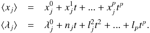 (19)The
mean elements are useful for
(19)The
mean elements are useful for
-
the determination of the starting integration constants in building classical planetary theories,
-
the determination of the integration constants of general planetary theories (Laskar 1988),
-
the amelioration of general planetary theories by fitting the long-period terms of these theories to the mean elements of classical theories (Bretagnon & Simon 1990).
The purpose of the mean elements is not to compute ephemerides. Nevertheless, it is
possible to obtain approximate ephemerides of the planets by adding the small Poisson
series of μ given by Simon et al.
(1994) to the mean elements. For the heliocentric longitudes, the precision of
these approximate ephemerides is about a few arcseconds for the telluric planets and
Neptune and about a few tens of arcseconds for the other planets over the time span from
1000 to 3000. Mean elements are too voluminous to be published in this paper, but they are
available on the WEB server of the IMCCE. We give here only the integration constants
 and the mean
motions nj of the solutions VSOP2013 (Table
5) and TOP2013 (Table 6).
and the mean
motions nj of the solutions VSOP2013 (Table
5) and TOP2013 (Table 6).
7.2. Number of terms of the series
We give the number of terms of the solutions VSOP2013 and TOP2013, for different levels of truncation in the series, in Table 7. For the small levels of truncation, the TOP solutions are more compact than the VSOP solutions for the major planets. This is due both to the best convergence of the Poisson series in the TOP representation and because numerous VSOP terms of a period superior to 1000 yrs are represented in TOP by the same small multiples of μ (smaller than 17μ).
Number of terms of the solutions VSOP2013 and TOP2013 for several levels of truncation.
7.3. Precision over the time span from 1890 to 2000
7.3.1. VSOP solutions
We have estimated the precision of VSOP2013 and VSOP2010 by computing their maximum differences to INPOP10a and DE405 from 1890 to 2000. Table 8 gives these differences for the elliptic elements of the eight planets. This table also gives the differences between VSOP2000 and DE403 given by Moisson & Bretagnon (2001). The accuracy of VSOP2013 is very good. The precision of the mean longitudes is about a few 0.01 mas for Mercury, Venus, EMB, Saturn, and Neptune, 0.2 mas for Jupiter, and 0.7 mas for Mars and Uranus. Related to VSOP2000, the improvement is about a factor of 2 for Uranus and up to 24 for EMB and Neptune. This is especially the result of the better inclusion of the perturbations by the asteroids and Pluto. Moreover, we note that the VSOP2013-INPOP10a differences are smaller than the VSOP2010-DE405 differences by a factor of 2.5 to 5 for the planets from Mercury to Jupiter. The reason is that the computation of the perturbations by the asteroids is closer between VSOP2013 and INPOP10a than in the case of VSOP2010 and DE405 as explained in Sect. 6.2. Another estimation of the precision of our solutions is given in Table 9 which gives the accuracy of VSOP2013, VSOP2010, and VSOP2000 compared to the first version VSOP82 (Bretagnon 1982) for the mean longitudes of planets from 1890 to 2000. We can see that the improvement is very important for the new VSOP solutions, especially for VSOP2013 (by a factor between 15 and 2121).
The differences between VSOP2013 and INPOP2010a for the mean longitudes of the planets from 1890 to 2000 are illustrated by Fig. 1.
Maximum differences from 1890 to 2000 between VSOP2013, VSOP2010, VSOP2000, and the numerical integrations for the elliptic variables.
Mean longitudes of the planets: gain in precision with respect to VSOP82 for VSOP2013, VSOP2010, and VSOP2000 from 1890 to 2000.
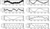 |
Fig. 1 Mean longitudes of the planets: VSOP2013 − INPOP10a differences from 1890 to 2000. Units are in mas. |
7.3.2. TOP solutions
The Table 10 gives the differences between
TOP2013 and INPOP10a, and between TOP2010 and DE405 for the ecliptic elements of the
four major planets and Pluto from 1890 to 2000. The orbits of the telluric planets are
not integrated with the major planets and the TOP theories cannot be as accurate as the
VSOP theories over short time spans. Nevertheless, we can see that TOP2013 is more
precise than TOP2010 thanks to the method used for computing the perturbations by the
telluric planets in TOP2013 as explained in Sect. 4.2.3. The precision of TOP2013 is of
the same order as the precision of VSOP2000. For Pluto, over the time span from 1890 to
2000, the accuracy is about 3 mas for the mean longitude, about 125 km for
a, and 2 × 10⁻⁸ for k and
h. This accuracy is far below the actual uncertainties of the Pluto
observations. The differences between TOP2013 and INPOP2010A for the mean longitude of
Pluto from 1890 to 2000 are illustrated in Fig. 2.
We see that these differences are short-period terms. Although, the short-period terms
perfectly converge in the iterative process, the bad convergence of the perturbations
corresponding to the argument  (see Sect. 5.3.4) involves an uncertainty in the determination of the integration
constants explaining these short-period differences.
(see Sect. 5.3.4) involves an uncertainty in the determination of the integration
constants explaining these short-period differences.
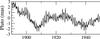 |
Fig. 2 Mean longitude of Pluto: TOP2013 − INPOP10a differences from 1890 to 2000. Units are in mas. |
Maximum differences from 1890 to 2000 between TOP2013, TOP2010, and the numerical integrations for the elliptic variables.
7.4. Precision over large time spans
The accuracy of our solutions over large time spans has been estimated by computing the differences with two numerical integrations from −4000 to 8000. The solutions VSOP2010 and TOP2010 have been compared with an internal numerical integration, the initial values of which are issued from the solutions. The solutions VSOP2013 and TOP2013 have been compared with the extension of INPOP10a from −4000 to 8000 (Manche 2012, priv. comm.). The comparisons with these two different integrations are similar. Tables 11 and 12 refer only to the comparisons with the extension of INPOP10a.
7.4.1. Telluric planets
Table 11 gives the differences between VSOP2013 and the extension of INPOP10a from −4000 to 8000 (Manche 2012, priv. comm.) for the mean longitude (λ) and the heliocentric coordinates (L, B, R) of the four telluric planets over three time spans: from 900 to 3100, from 0 to 4000, and from −4000 to 8000.
We can see that the precision remains good for large time spans. For instance, from 0 to 4000, the accuracy of the heliocentric longitude is better than 0.02″ for Venus and 0.05″ for Mercury and EMB. From −4000 to 8000, the precision is better than 0.2″ for Mercury and Venus, about 1″ for EMB and 1.7″ for Mars. The improvement is about a factor of 5 compared to VSOP2000. However, we see that the precision decreases with time more quickly for EMB and Mars than for Mercury and Venus. This is due to the perturbations by the asteroids which should be computed at the second order of masses to improve the accuracy of the solutions of the motion of these two planets over large time spans.
The differences between VSOP2013 and INPOP10a for the heliocentric longitudes of the telluric planets from −4000 to 8000 are illustrated in Fig. 3.
Telluric planets: maximum differences over large time spans between VSOP2013 and the extension of INPOP10a from −4000 to 8000 for the mean longitude and the heliocentric coordinates.
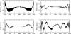 |
Fig. 3 Heliocentric longitudes of the telluric planets: differences between VSOP2013 and the extension of INPOP10a from −4000 to 8000. Units are in arcsecond . |
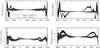 |
Fig. 4 Heliocentric longitudes of the major planets: differences between TOP2013 and the extension of INPOP10a (straight lines) and between VSOP2013 and the extension of INPOP10a (dotted lines) from −4000 to 8000. Units are in arcseconds. |
7.4.2. Major planets and Pluto
Table 12 gives, for the major planets and Pluto, the differences between VSOP2013, TOP2013, and the extension of INPOP10a for the same variables and the same time spans as in Table 11. For Jupiter and Saturn and for the time span from −4000 to 8000, the second line of VSOP corresponds to the theory without the corrections from TOP2013. We see that the improvement due to the supplementary material from TOP2013 is about a factor of 5 for the mean and heliocentric longitudes of these two planets. From −4000 to 8000, the precision of the heliocentric longitudes of the major planets is included between 1″ and 5″ for Jupiter, Uranus, and Neptune and about 11″ for Saturn. This represents an improvement compared to VSOP2000 of a factor of 5 to 10.
Nevertheless, TOP2013 remains the more precise solution over large time spans. From −4000 to 8000, the precision of the heliocentric longitudes of the major planets is about 0.4″ for Jupiter, 0.7″ for Uranus and Neptune, and 0.9″ for Saturn. The gain in precision, compared to VSOP2013, is between 10 and 15 for Jupiter and Saturn and between 1.5 and 4 for Uranus and Neptune. The differences between VSOP2013, TOP2013, and the extension of INPOP10a for the heliocentric longitudes of the major planets from −4000 to 8000 are illustrated in Fig. 4.
For Pluto, the precision remains good from 900 to 3100 (about 0.8″ for the heliocentric longitude) and still correct from 0 to 4000 (about 12″). For larger time spans, the precision quickly decreases, but the existence of a libration of the longitude of Pluto, with a period about 19 900 yrs (Milani et al. 1989), means that we cannot hope to build an analytical solution of Pluto valid over time spans greater than a few thousand years.
Major planets and Pluto: maximum differences over large time spans between VSOP2013, TOP2013, and the extension of INPOP10a from −4000 to 8000.
7.5. The solutions on the WEB server of the IMCCE
7.5.1. The VSOP2013 solution2
For VSOP2013, we give on the WEB server of the IMCCE:
-
The complete Poisson developments of the elliptic variables of the eight planets and Pluto.
-
Developments in the form of Tchebychev polynomials for the heliocentric rectangular coordinates (positions and velocities) of the eight planets over different time spans.
-
The mean elements of the elliptic variables of the eight planets.
-
Subroutines for reading the developments and computing the coordinates for given values of time.
7.5.2. The TOP2013 solution3
The TOP2013 solution is much more compact than VSOP2013 and it is not necessary to use developments under the form of Tchebychev polynomials. So, we give:
-
The complete Poisson developments of the elliptic variables (four major planets and Pluto) and of the heliocentric spherical and rectangular variables (four major planets).
-
The mean elements of the elliptic variables of the four major planets and Pluto.
-
Subroutines for reading the developments and computing the coordinates for given values of time.
7.6. Possible improvements
Some improvements of the theories can still be made.
For VSOP2013, it would be possible
-
to improve the accuracy of the motion of the telluric planets (specially EMB and Mars) over large time spans by computing the perturbations of the asteroids on the planets to the second order of masses;
-
to improve the accuracy of the motion of Jupiter and Saturn over large time spans by developing the Poisson series up to the 20th degree with respect to time;
-
to improve the accuracy of the relativistic corrections, using the techniques suggested by Brumberg (2012).
The TOP2013 theory could be more accurate by improving the modelling of the perturbations due to the telluric planets. Integrating the motion of the telluric planets in the iterative process would not be easy because the computation of very short periods in the motion of Mercury would lead to important difficulties in the harmonic analysis. A better method would be to do two kinds of iterations in the VSOP process, one with the telluric planets, another without. The difference between the two processes should give a good estimation of the perturbations of the telluric planets on the outer planets.
8. Conclusion
The new analytical theories VSOP2013 and TOP2013 built at the IMCCE are complementary and have been greatly enhanced since the previous versions. They are fitted to INPOP10a, a numerical integration of the motion of the planets that takes into account more recent observations. The VSOP2013 theory is the best analytical theory for the motion of the eight solar system planets over time spans of a few hundred years. The improvement over VSOP2000 is about a factor of 2 for Uranus, 5 for Mars and Jupiter, and greater than 10 for the other planets. Moreover, VSOP2013 remains very accurate over large time spans for the motion of the telluric planets. The TOP2013 theory was developed in a compact and easy to use form. It is the most precise theory for the motion of the four major planets over large time spans; TOP2013 also gives a solution of the motion of the Pluto-Charon barycenter with good accuracy up to time spans of a few thousand years.
Lastly, the subroutines used to build VSOP2013 and TOP2013 are ready to fit these theories to new versions of INPOP.
The word “theory” is a traditional term used in celestial mechanics for the analytical solution of the equations of the motion of solar system bodies.
Acknowledgments
We dedicate this paper to the memory of Pierre Bretagnon who was the initiator of the VSOP theories and who devoted all his energy and his talent to the development of planetary analytical solutions for over thirty years. We thank the referee, Elena Pitjeva, for the helpful improvement she proposed to the original manuscript.
References
- Bretagnon, P. 1982, A&A, 114, 278 [NASA ADS] [Google Scholar]
- Bretagnon, P., & Francou, G. 1988, A&A, 202, 309 [Google Scholar]
- Bretagnon, P., & Simon, J.-L. 1986, Planetary programs and tables from −4000 to +2800 (Richmond: Willmann-Bell) [Google Scholar]
- Bretagnon, P., & Simon, J.-L. 1990, A&A, 239, 387 [NASA ADS] [Google Scholar]
- Brumberg, V. A. 2012, Notes scientifiques et techniques de l’Institut de Mécanique céleste S096, 1 [Google Scholar]
- Chapront, J., Bretagnon, P., & Mehl, M. 1975, Celest. Mech., 11, 379 [NASA ADS] [CrossRef] [Google Scholar]
- Chapront, J., Chapront-Touzé, M., & Francou, G. 2002, A&A, 387, 700 [NASA ADS] [CrossRef] [EDP Sciences] [Google Scholar]
- Chapront-Touze, M., & Chapront, J. 1983, A&A, 124, 50 [NASA ADS] [Google Scholar]
- Fairhead, L., & Bretagnon, P. 1990, A&A, 229, 240 [NASA ADS] [Google Scholar]
- Fienga, A., & Simon, J.-L. 2005, A&A, 429, 361 [NASA ADS] [CrossRef] [EDP Sciences] [Google Scholar]
- Fienga, A., Manche, H., Laskar, J., & Gastineau, M. 2008, A&A, 477, 315 [NASA ADS] [CrossRef] [EDP Sciences] [Google Scholar]
- Fienga, A., Laskar, J., Morley, T., et al. 2009, A&A, 507, 1675 [NASA ADS] [CrossRef] [EDP Sciences] [Google Scholar]
- Fienga, A., Laskar, J., Kuchynka, P., et al. 2011, Cel. Mech. Dyn. Astron., 111, 363 [Google Scholar]
- Folkner, W. M. 2010, JPL Interoffice Memorandum, 343, R [Google Scholar]
- Folkner, W. M., Williams, J. G., & Boggs, D. H. 2009, Interplanetary Network Progress Report, 178, C1 [Google Scholar]
- Irwin, A. W., & Fukushima, T. 1999, A&A, 348, 642 [NASA ADS] [Google Scholar]
- Joutel, F. 1990, Thèse de doctorat, Observatoire de Paris [Google Scholar]
- Laskar, J. 1988, A&A, 198, 341 [NASA ADS] [Google Scholar]
- Milani, A., Nobili, A. M., & Carpino, M. 1989, Icarus, 82, 200 [NASA ADS] [CrossRef] [Google Scholar]
- Moisson, X., & Bretagnon, P. 2001, Celest. Mech. Dyn. Astron., 80, 205 [Google Scholar]
- Pitjeva, E. V. 2005, Solar System Research, 39, 176 [Google Scholar]
- Pitjeva, E. V. 2010, in IAU Symp. 261, eds. S. A. Klioner, P. K. Seidelmann, & M. H. Soffel, 170 [Google Scholar]
- Simon, J. L. 1983, A&A, 120, 197 [NASA ADS] [Google Scholar]
- Simon, J. L. 1986, Notes scientifiques et techniques de l’Institut de Mécanique céleste S005, 1 [Google Scholar]
- Simon, J. L. 2004, Notes scientifiques et techniques de l’Institut de Mécanique céleste S081, 53 [Google Scholar]
- Simon, J. L., & Bretagnon, P. 1984, A&A, 138, 169 [NASA ADS] [Google Scholar]
- Simon, J.-L., & Joutel, F. 1988, A&A, 205, 328 [NASA ADS] [Google Scholar]
- Simon, J. L., Joutel, F., & Bretagnon, P. 1992, A&A, 265, 308 [NASA ADS] [Google Scholar]
- Simon, J. L., Bretagnon, P., Chapront, J., et al. 1994, A&A, 282, 663 [NASA ADS] [Google Scholar]
- Standish, Jr., E. M. 1982, A&A, 114, 297 [NASA ADS] [Google Scholar]
- Standish, E. 1998, JPL Interoffice Memorandum, 312, F.98 [Google Scholar]
- Standish, E., Newhall, X., Williams, J., & Folkner, W. 1995, JPL Interoffice Memorandum, 314, 10 [Google Scholar]
All Tables
GM of the Sun, the planets, and the five big asteroids used for the construction of INPOP10a.
Poisson developments of the mean longitude of Jupiter for the argument 4λ5 − 10λ6 for VSOP2013, TOP2013, TOP2013 in VSOP form, and corrections to VSOP2013.
Perturbations at the first order of the masses for the mean longitudes greater than 5 × 10-11 rad: comparison between Saturn perturbed by Jupiter and Pluto perturbed by Uranus.
Number of terms of the solutions VSOP2013 and TOP2013 for several levels of truncation.
Maximum differences from 1890 to 2000 between VSOP2013, VSOP2010, VSOP2000, and the numerical integrations for the elliptic variables.
Mean longitudes of the planets: gain in precision with respect to VSOP82 for VSOP2013, VSOP2010, and VSOP2000 from 1890 to 2000.
Maximum differences from 1890 to 2000 between TOP2013, TOP2010, and the numerical integrations for the elliptic variables.
Telluric planets: maximum differences over large time spans between VSOP2013 and the extension of INPOP10a from −4000 to 8000 for the mean longitude and the heliocentric coordinates.
Major planets and Pluto: maximum differences over large time spans between VSOP2013, TOP2013, and the extension of INPOP10a from −4000 to 8000.
All Figures
|
Fig. 1 Mean longitudes of the planets: VSOP2013 − INPOP10a differences from 1890 to 2000. Units are in mas. |
| In the text | |
|
Fig. 2 Mean longitude of Pluto: TOP2013 − INPOP10a differences from 1890 to 2000. Units are in mas. |
| In the text | |
|
Fig. 3 Heliocentric longitudes of the telluric planets: differences between VSOP2013 and the extension of INPOP10a from −4000 to 8000. Units are in arcsecond . |
| In the text | |
|
Fig. 4 Heliocentric longitudes of the major planets: differences between TOP2013 and the extension of INPOP10a (straight lines) and between VSOP2013 and the extension of INPOP10a (dotted lines) from −4000 to 8000. Units are in arcseconds. |
| In the text | |
Current usage metrics show cumulative count of Article Views (full-text article views including HTML views, PDF and ePub downloads, according to the available data) and Abstracts Views on Vision4Press platform.
Data correspond to usage on the plateform after 2015. The current usage metrics is available 48-96 hours after online publication and is updated daily on week days.
Initial download of the metrics may take a while.