| Issue |
A&A
Volume 557, September 2013
|
|
|---|---|---|
| Article Number | A40 | |
| Number of page(s) | 16 | |
| Section | Stellar structure and evolution | |
| DOI | https://doi.org/10.1051/0004-6361/201321509 | |
| Published online | 23 August 2013 | |
Critically-rotating accretors and non-conservative evolution in Algols
Institut d’Astronomie et d’Astrophysique, Université Libre de Bruxelles, ULB, CP 226, 1050 Brussels, Belgium
e-mail: This email address is being protected from spambots. You need JavaScript enabled to view it.
Received: 19 March 2013
Accepted: 5 July 2013
Abstract
Context. During the mass-transfer phase in Algol systems, a large amount of mass and angular momentum are accreted by the gainer star, which can be accelerated up to its critical Keplerian velocity. The fate of the gainer once it reaches this critical value is unclear.
Aims. We investigate the orbital and stellar spin evolution in semi-detached binary systems, specifically for systems with rapidly rotating accretors. Our aims are to better distinguish between the different spin-down mechanisms proposed that can consistently explain the slow rotation observed in Algols’ final states and to assess the degree of non-conservatism due to the formation of a hotspot.
Methods. We use our state-of-the-art binary evolution code, Binstar, which incorporates a detailed treatment of the orbital and stellar spin and includes all torques due to mass transfer, the interactions between a star and its accretion disc, tidal effects, and magnetic braking. We also present a new prescription for mass loss due to the formation of a hotspot based on energy conservation.
Results. The coupling between the star and the disc via the boundary layer prevents the gainer from exceeding the critical rotation. Magnetic-field effects, although operating, are not the dominant spin-down mechanism for sensible field strengths. Spin down owing to tides is 2–4 orders of magnitudes too weak to compensate the spinning-up torque due to mass accretion. Moreover, we find that the final separation strongly depends on the spin-down mechanism. The formation of a hotspot leads to a large event of mass loss during the rapid phase of mass transfer. The degree of conservatism strongly depends on the opacity of the impacted material.
Conclusions. A statistical study and new observational constraints are needed to find the optimal set of parameters (magnetic-field strength, hotspot geometry, etc.) to reproduce Algol evolutions.
Key words: binaries: general / stars: rotation / accretion, accretion disks / stars: magnetic field / stars: evolution / methods: numerical
© ESO, 2013
1. Introduction
Algols are short orbital period (from several hours to tens of days) semi-detached binaries composed of a hot B-A main sequence star and a cool F-K giant star (Kopal 1955; Giuricin et al. 1983). Because of the small separation, the initially more massive star (henceforth, the donor) overfills its Roche lobe and matter then channels to the companion (the gainer) through the inner Lagrangian point ℒ1, by Roche lobe over-flow (RLOF). The duration of the mass-transfer phase (with rates reaching ≈10-4 M⊙ yr-1) is long enough (several 105 yrs) that a significant amount of mass can be accreted by the gainer (up to several solar masses). Observations clearly attest to the reversal of the mass ratio during RLOF with a donor star (now a giant) that is less massive than its main-sequence companion. The global evolution is well established, but many open questions, such as discrepancies between canonical simulations and observations about the final orbital periods and mass ratios (van Rensbergen et al. 2010b, 2011), still remain.
Previous numerical simulations of Algols (Nelson & Eggleton 2001; van Rensbergen et al. 2011) have provided a broad understanding of short-period binaries, focusing on some specific aspects, such as non-conservative mass transfer (Giannuzzi 1981) or the properties of the mass-transfer stream (Flannery 1975). Except for the study of Dervişoğlu et al. (2010), there are, however, basically no simulations that follow the angular-momentum evolution for both the stars and the orbit in detail, and that account for torques arising from tides, mass transfer, magnetic-field effects, disc accretion or direct impact, and spin-down mechanisms.
Moreover, the evolution of critically-rotating accretors is poorly understood: it is well known that the transferred mass carries enough angular momentum (Kruszewski 1967) to rapidly spin the gainer up to its critical spin-angular velocity (Packet 1981):  (1)For a typical 6 + 3.6 M⊙ system with initial period Pinit = 2.5 days in the absence of spin-down mechanisms, only 3 percent (0.12 M⊙) of the total amount of matter transferred by RLOF (more than 5 M⊙) is enough to spin the gainer up to the critical rotation. However, it is not clear whether the gainer reaches the critical velocity, whether it is spun down due to any braking mechanisms, or if accretion stops (de Mink et al. 2007). Many physical processes have been proposed to spin down the gainer, including tides (Zahn 1977), magnetic braking (Armitage & Clarke 1996; Stȩpień 2000; Dervişoğlu et al. 2010), or the limitation of the accretion of angular momentum through the interaction with an accretion disc (Popham & Narayan 1991; Paczynski 1991; Colpi et al. 1991; Bisnovatyi-Kogan 1993). However, none of these processes have been applied to a binary-star evolution code that consistently follows the stellar spin velocity and all torques owing to mass accretion and mass loss.
It has also been shown that some Algol systems must be non-conservative to comply with observations of mass ratios (for example Refsdal et al. 1974; Massevitch & Yungelson 1975; Mezzetti et al. 1980; Sarna 1993; Nelson & Eggleton 2001). Yet, only mass loss through the outer Lagrangian point ℒ3 (Sytov et al. 2007), bipolar jets (Ak et al. 2007) or hotspot formation (van Rensbergen et al. 2011) have been proposed to account for this kind of evolution. Non-conservative mass transfer in stellar evolution codes is generally treated via a free parameter, defining the amount of matter accreted by the gainer star compared to the amount of matter passing through the inner Lagrangian point (de Greve 1993; Sarna et al. 1998; Eggleton & Kiseleva-Eggleton 2002; Dervişoğlu et al. 2010).
In this article, we focus on the evolution of the gainer’s spin-angular velocity and non-conservative evolution. To do so, we study a specific case B mass-transfer system (M1 = 3.6 M⊙, M2 = 6 M⊙, and Porb = 2.5 days) in which the donor is a hydrogen-shell burning star. Mass transfer starts just after the star leaves the main sequence, and the rate is characterised by a short phase of rapid mass transfer (hereafter rapid phase) where most of the mass is transferred, followed by a long-lasting slow phase (hereafter quiescent phase) where most of the orbital-separation changes take place.
To address the aforementioned problems (i.e., critical rotation of the gainer and non-conservative evolution), we used the binary-star evolution code Binstar (Siess et al. 2013). Section 2 presents the implemented binary input physics; our treatment of rotation and the various spin-down mechanisms and the torques due to magnetic fields, star-disc interactions, and tides. We also describe our implementation of the hotspot physics and its consequences on the mass accretion rate. In Sect. 3, we apply these prescriptions to our specific Algol system and analyse the effect of each torque on the gainer’s spin. A calculation with a hotspot configuration is also presented. In Sect. 4, observational constraints for Algol systems and related objects are discussed, and their impact on the spin-down mechanism investigated. Finally, we discuss the effect of non-conservative evolution on the close environment of the system (i.e., the region impacted by the system mass-loss) and examine the limitations of our assumptions regarding solid-body rotation and disc formation. The conclusions are given in Sect. 5.
2. The Binstar code
Binstar is an extension of the 1-dimensional stellar evolution code Starevol (Siess 2006) that handles the simultaneous calculation of the binary orbital parameters (separation and eccentricity) and the two stellar components. A complete description of the code can be found in Siess et al. (2013).
In this section, we outline our treatment of stellar rotation and the effects of mass transfer on the stellar spins. We specially focus on the torque due to magnetic fields and the formation of a star-disc boundary layer. Hereafter, the subscripts “g” and “d” refer to the gainer (primary star in Algol systems) and donor (secondary star), respectively. The models presented hereafter assume solid-body rotation. The limitations associated with this assumption are discussed in Sect. 4.3.
The RLOF mass-transfer rate follows the prescriptions described by Ritter (1988) and Kolb & Ritter (1990). In their formalism, two regimes have been considered, depending on whether the Roche radius lies in the optically thick or thin layers of the donor star.
Let us finally emphasize that the (solid) rotation profile and all the torques are computed at each iteration during the convergence process, along with the evolution of the separation and mass transfer rates. This procedure brings numerical stability and ensures that the calculation of the orbital elements are in step with the stellar structures.
2.1. Treatment of angular momentum in BINSTAR
Binstar follows the angular-momentum evolution of each star and the orbit. The total angular momentum of the system (JΣ) is given by  (2)where Jd,g are the stellar spin-angular momenta and Jorb is the orbital component, such that
 ![Mathematical equation: \begin{equation} J_{\mathrm{orb}}=M_{\mathrm{d}}M_{\mathrm{g}}\left[\frac{Ga(1-e^{2})}{M_{\Sigma}} \right]^{1/2} , \label{eq:jorb} \end{equation}](/articles/aa/full_html/2013/09/aa21509-13/aa21509-13-eq18.png) (3)where a is the binary separation, e is the eccentricity, and MΣ = Md + Mg is the total mass of the system. Evolution is conservative if MΣ and JΣ are constant during the evolution. The conservation of angular momentum implies that
(3)where a is the binary separation, e is the eccentricity, and MΣ = Md + Mg is the total mass of the system. Evolution is conservative if MΣ and JΣ are constant during the evolution. The conservation of angular momentum implies that  (4)where
  are the torques applied on each star,
  is the rate of change of the orbital angular momentum, and
  represents the angular-momentum loss rate by the system in non-conservative evolution. Torques from mass transfer and tides are explained in detail in Siess et al. (2013) and summarised in Table 1.
Summary of the angular-momentum transfer rates involved in a non-conservative system (β < 1).
2.2. Magnetic torques
Depending on its configuration, a magnetic field can either spin the star up or down. We consider two effects: magnetic-wind braking and disc-locking.
2.2.1. Magnetic-wind braking
Stars expel matter through winds. Assuming the specific angular momentum of the surface layers of the star to be  (5)this matter removes angular momentum at a rate
  (6)where ṀW is the wind mass-loss rate, R∗ is the stellar radius, and Ω∗ is its spin-angular speed. If the magnetic field co-rotates with the star, particles emitted by the wind can either be trapped within the dead zone (where the magnetic-field lines are closed) or leave the system by flowing along open magnetic-field lines up to the Alfvèn radius RA (Weber & Davis 1967; Mestel 1968). Beyond RA where the wind speed equals the Alfvèn speed, matter decouples from the magnetic field and particles can freely escape the system. The angular-momentum loss rate at RA is given by
  (7)The torque is efficient because RA ≫ R∗ and can be written as (e.g. Dervişoğlu et al. 2010)
 ![Mathematical equation: \begin{equation} \dot{J}_{\mathrm{loss,*}}^{\mathrm{wind,}\vec{B}} =- \left[\vert \dot{M}_{\mathrm{W}}\vert^{(4m-9)}B_{*}^{8}(2 G M_{*})^{-2} R_{*}^{8m}\right]^{1/(4m-5)}\Omega_{*}, \label{eq:mdot_wind} \end{equation}](/articles/aa/full_html/2013/09/aa21509-13/aa21509-13-eq70.png) (8)where m is a parameter characterising the topology of the magnetic field of magnitude B∗ at the stellar surface. For our purpose, we assume a bipolar configuration (m = 3), which is a reasonable approximation around the Alfvèn radius where the matter is released (Livio & Pringle 1992). In our models, only the magnetic-field strength B∗ is left as a free parameter. The wind mass-loss rate is determined using the prescription of Reimers (1975). In a case study, we also considered a rotationally enhanced wind mass loss where the modified rate is given by (Maeder & Meynet 2001)
(8)where m is a parameter characterising the topology of the magnetic field of magnitude B∗ at the stellar surface. For our purpose, we assume a bipolar configuration (m = 3), which is a reasonable approximation around the Alfvèn radius where the matter is released (Livio & Pringle 1992). In our models, only the magnetic-field strength B∗ is left as a free parameter. The wind mass-loss rate is determined using the prescription of Reimers (1975). In a case study, we also considered a rotationally enhanced wind mass loss where the modified rate is given by (Maeder & Meynet 2001)  (9)where Γ is the ratio of the stellar luminosity over the Eddington luminosity (Eq. (35)), ρm the stellar mean density
  (10)and α a force multiplier such that α = 0.52, 0.24, 0.17 and 0.15 for log (Teff ≥ 4.35, 4.30, 4.00 and 3.90) respectively (Lamers et al. 1995).
2.2.2. Disc-locking
If an accretion disc is present, the gainer’s magnetic field anchors into it. Since the disc does not co-rotate with the star, magnetic-field lines are twisted, creating a toroidal magnetic-field component that generates a torque on the star. If the magnetic field is anchored beyond the co-rotation radius Rco, defined as  (11)then the torque is negative and the star is spun down. The inner disc is truncated at the Alfvén radius RA, because the magnetic pressure is higher than the gas pressure below this region.
We assume a simple power law for the magnetic-field strength of the form B(r) = B∗(R∗/r)m for r > RA, considering the same magnetic-field geometry parameter as before (m = 3 for a bipolar configuration). The resulting torque is given by (Armitage & Clarke 1996)  (12)with
  . Depending on the location of Rco and RA, the global torque can be either positive or negative and is most efficient at spinning-down the gainer when RA = Rco because there are no regions of the disc that rotate faster than the star (remember that below RA the disc is truncated) in this configuration. The expression of this maximum torque (Stȩpień 2000) is given by
  (13)and does not depend on the disc properties, such as its mass.
2.3. Tidal effects
Tides have two effects on a binary system: they circularise the orbit of eccentric systems and synchronise the stellar spin with the orbital period. The implementation of tides in Binstar follows the prescription described by Zahn (1977) and includes the Zahn (1989) refinement for convective stars in short-period systems (see Siess et al. 2013, for details).
2.4. Accretion disc and star-disc boundary layer
The matter-stream escaping the donor through the ℒ1 point will free-fall into the gainer’s potential well. If the stream’s minimum distance of approach to the gainer is such that Rmin > Rg, then the stream will orbit the gainer until it collides with itself. Subsequently, collisions between particles lead to the formation of a ring at the circularisation radius. The matter will then spread out, and an accretion disc forms (Kruszewski 1967; Lubow & Shu 1975).
The properties of accretion discs around fast-rotating stars have been widely studied (e.g., Paczynski 1991; Popham & Narayan 1991; Colpi et al. 1991; Bisnovatyi-Kogan 1993). Their 1D calculations show that accretion does not stop when the gainer reaches its critical velocity because of the presence of a boundary layer between the star and the disc. The physics of this boundary and its implementation in Binstar are presented in the next section.
2.4.1. The Paczynski model
The main idea of this model (Paczynski 1991) is to assume that the star and the disc behave as one fluid. A polytropic equation of state is used for both the disc and the star with the pressure given by  (14)where K and n are two constants. The hydrostatic equilibrium of the disc is ensured by balancing the gravitational acceleration, centrifugal acceleration, and pressure gradient (in a cylindrical coordinate system in which r is the distance from the rotation axis and z the distance from the equatorial plane); that is,
 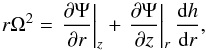 (15)where z = h(r) is the disc thickness as a function of r, Ω is the disc angular velocity and
 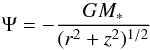 (16)is the gravitational potential of a point mass with M∗ being the stellar mass. For a thin disc [h(r) ≪ r], the equation of hydrostatic equilibrium in the z-direction is
 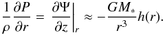 (17)After some algebra and using Eq. (15), the condition for hydrostatic equilibrium may be re-written as
 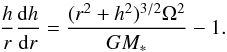 (18)The second equation expressing the angular-momentum conservation is written as
  (19)where Ṁ is the mass flux in the disc, j is the specific angular momentum carried with the disc material, and Γ is the torque due to viscous stresses inside the disc. Using the polytropic equation of state, the α-prescription for the disc viscosity (Shakura & Sunyaev 1973), and the equation of the torque acting between two cylinders in a differentially rotating disc (Pringle 1981), Eq. (19) is rewritten as (Paczynski 1991)
 ![Mathematical equation: \begin{equation} \label{eq:bl_AM_balance} \left[ 4\pi \alpha \frac{(G M_{*})^{n+1/2}}{K^{n}}\right]\frac{\mathrm{d} \Omega}{\mathrm{d} r} = \frac{r^{3n-3/2}}{z^{2n+3}}(\dot{J} - \dot{M}r^{2} \Omega). \end{equation}](/articles/aa/full_html/2013/09/aa21509-13/aa21509-13-eq106.png) (20)
(20)
2.4.2. Dimensionless equations
For convenience, the dimensionless variables are introduced:
 where Ω∗ and Ωcrit are the stellar and critical angular velocities, respectively. We also define the two constants:
  (23)and
  (24)where j∗ represents the specific angular momentum of the disc material at the effective stellar radius R∗, which is defined as (Chandrasekhar 1939)
 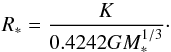 (25)Following Paczynski (1991), we use ς = 106 throughout the computations. In dimensionless form, Eqs. (18) and (20) can be re-expressed as
 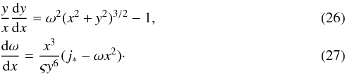 This system of equations does not depend on the disc properties, such as mass or radial extent. This system is solved using a two-point boundary value solver (Capper et al. 2007). For numerical reasons, two sets of boundaries are used depending on the stellar spin-angular velocity.
For rapidly rotating stars with ω∗/ωcrit ≈ 1, the structure of the disc must satisfy the boundary condition  (28)where rtr = 0.8rpolar is an arbitrary transition radius between the star and the disc, and rpolar is the star’s polar radius.
For slowly rotating stars, the spin-angular velocity profile presents a local maximum in the boundary layer. This maximum, which is located at a radius rnt, corresponds to a zero-torque condition between the star and the disc. The inner boundary condition is written as  (29)A Runge-Kutta integrator (Press et al. 2007) is used to solve the inner part of the system between rnt and rtr.
For both rapidly and slowly rotating systems, the outer boundary condition is  (30)where ωKepler is the Keplerian angular speed at the outer edge of the disc. Details on the method of calculation can be found in Paczynski (1991).
The solution of this system of equations provides the value of the specific angular momentum jdisc = j∗ accreted by the star as a function of its stellar spin. The torque exerted on the star is then  (31)where
  is the mass accretion rate for the gainer star. Note that jdisc can be negative.
To ease the computation when the star is not critically rotating (less than 80% of the critical spin), the accreted specific angular momentum can be set as a fraction fjdisc of the Keplerian specific angular momentum at the surface of the star; that is,  (32)We use fjdisc = 1, which is the mean value computed with the “boundary-layer” mechanism for non-critically rotating accretors.
In the disc, advection of matter occurs due to the transport of angular momentum by viscosity. By treating the star-disc boundary layer as one fluid, the same mechanism also applies at the stellar surface: when the star reaches critical rotation, the accretion of angular momentum is no longer possible, and viscous processes remove spin-angular momentum from the star, keeping it at a critical value but not exceeding it. This mechanism allows the star to accrete large amounts of mass, while giving angular momentum back to the disc. This extra angular momentum leads to the spreading of the disc. The outer disc radius is truncated because of tidal interaction between the disc and the donor star (Lin & Papaloizou 1979; Whitehurst 1988; Ichikawa & Osaki 1994) and, consequently, some angular momentum is returned to the orbit.
2.5. Direct impact and hotspot formation
A second mode of mass transfer occurs when Rmin < Rg, such that the stream impacts the gainer’s surface (hereafter “direct impact”). In this case, we follow the evolution of the stream through a ballistic approach to determine the precise location, velocity, and angular momentum of the impacting stream (Huang 1963; Kruszewski 1964; Flannery 1975).
When the particle collides with the star, its specific angular momentum is  (33)where r and v are respectively the radius vector of the particle from the gainer’s stellar centre, and the particle velocity at the impact location. These are determined by integrating the equations of motion of the particle using a Runge-Kutta scheme. Using Eq. (33), the torque applied on the accretor is given by
  (34)When the stream impacts the star (or the disc’s outer radius), its kinetic energy is converted into thermal energy and a hotspot forms (Peters & Polidan 2004; Lomax et al. 2012). If the hotspot luminosity exceeds the Eddington value such that
  (35)where κ is the plasma opacity, the matter escapes the system. We show in Appendix A (all quantities entering Eq. (36) being defined there) that if the mass-transfer rate exceeds
  (36)the evolution becomes non-conservative (Eggleton 2000; van Rensbergen et al. 2008). We use a prescription for
  , depending only on the total mass of the system and based on observations (see Appendix A, Eq. (A.20)).
The parameter β defining the fraction of the transferred mass that escapes the system is given by  (37)where
  . Note that the wind mass-loss contribution is not included.
In short-period binaries, matter may also escape the system through the third Lagrangian point (Sytov et al. 2007) at a rate of approximately 10-10 M⊙ yr-1, which is higher than stellar winds but still negligible compared to the RLOF mass-transfer rate. We neglect this aspect in our present investigation.
3. Results
In this section, we present new calculations of Algol evolution, considering the previously described spin-down mechanisms and non-conservative evolution. Our reference system is a 6 M⊙ + 3.6 M⊙ with an initial period of 2.5 days. Both stars are initially relaxed on the zero-age main sequence with composition Xg = 0.735 and Xd = 0.695 and are synchronised with the orbit. Initial effective temperatures (luminosities) are ≈10 500 K (≈130 L⊙) for the gainer and ≈19 500 K (≈1030 L⊙) for the donor. In this study, we do not consider Bondi-Hoyle accretion (![Mathematical equation: \hbox{$\dot{J}_{\mathrm{acc,[g,d]}}^{\mathrm{wind}}$}](/articles/aa/full_html/2013/09/aa21509-13/aa21509-13-eq147.png) , see Table 1) because of its negligible impact compared to RLOF mass transfer. By default, no spin-down mechanisms are used unless mentioned.
, see Table 1) because of its negligible impact compared to RLOF mass transfer. By default, no spin-down mechanisms are used unless mentioned.
3.1. On the spin up of the gainer
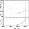 |
Fig. 1 Evolution of the mass-transfer rate (top), stellar masses (middle), surface velocity (bottom) for a 6 M⊙ donor (solid black line), and 3.6 M⊙ gainer (dotted red line) system with initial period Pinit = 2.5 days. |
Figure 1 shows the evolution of the mass-transfer rate (top panel), stellar masses (middle panel), and the surface-spin velocity of the gainer (in units of the critical Keplerian velocity; bottom panel) for our reference system, undergoing case B mass transfer. Here, we have not considered any spin-down mechanisms and have assumed fully conservative mass transfer. Mass and angular-momentum losses from the system only occur via winds (quasi-conservative evolution).
During the rapid phase, the mass-accretion rate reaches values up to 10-4 M⊙ yr-1, and by about 3 × 10⁴ years, the gainer reaches critical velocity (blue vertical line in Fig. 1). At this point, we stop the evolution. During this period, only a low amount of matter is transferred, and the gainer’s mass increases by 0.12 M⊙, which represents 3% of its initial mass (Fig. 1, middle panel). However, more than 5 M⊙ would have been transferred if the evolution was continued.
3.2. Effect of magnetic fields
The efficiency of magnetic-wind braking strongly depends on the mass-loss rate of the gainer (and on the parameter β for non-conservative evolution to a certain extent), and on | B∗ |. In the following simulations, we assume that the disc-locking activates as soon as the gainer is spun up and is at work even if direct impact is expected. Although contradictory, this assumption does not conflict with an observation of binaries in which the gainer is surrounded by a disc, even though the Lubow & Shu (1975) criterion1 implies direct impact (see Sect. 4.2.2).
The top panel of Fig. 2 shows the evolution of the gainer’s surface spin-angular velocity (normalised to the critical value) for different values of | B∗ |, where we consider both magnetic-wind braking and disc-locking. Only a magnetic field of intensity | B∗ | ≳ 3 kG can spin down the star sufficiently to prevent critical rotation.
 |
Fig. 2 Evolution of the gainer’s surface velocity (normalised to the critical velocity) for different spin-down mechanisms for our 6 + 3.6 M⊙ system with an initial period Pinit = 2.5 days. The horizontal line represents the critical spin-angular rotation of the star. All simulations are stopped when Ωsurf ≈ Ωcrit. Top panel: solid black line (labelled “Ref.”): | B∗ | = 0 kG, no braking mechanism; dotted red line (labelled “B.-L.”): boundary-layer mechanism, no magnetic field; dashed green line: Zahn (1989) tidal effect treatment only; long-dashed blue line: magnetic braking with | B∗ | = 3 kG. Bottom panel: solid black line: magnetic braking with | B∗ | = 1 kG; dotted red line: magnetic braking with | B∗ | = 2 kG; dashed green line (labelled M.-W.): magnetic-wind braking only with | B∗ | = 3 kG; long-dashed blue line (labelled D.-L.): disc locking only with | B∗ | = 3 kG. |
In the lower panel of Fig. 2, we present the evolution of the normalised spin-angular velocity for each magnetic-braking mechanism individually. As shown, wind braking is very inefficient, but various effects can contribute to strengthen its action. First, rotation can substantially enhance the mass loss rate because of the reduced gravity. To quantify this effect, we ran additional simulations using Eq. (9) for the wind loss rate. Although the mass-loss rate is increased by a factor of almost 3, the 2 kG configuration still produces a critically rotating gainer, and in the 3 kG case, the difference in stellar spin is insignificant, of the order of 2 percents. Therefore, change in the wind rate due to rotation has a negligible impact because disc-locking is so efficient (and independent of mass loss rate). Alternatively, Tout & Pringle (1992) argue that the dynamo process at the origin of the magnetic-field generation can enhance the mass loss rate and hence, the magnetic torque. Moreover, the evolution may not be conservative and some mass may leave the system from the hotspot (see Sects. 3.6 and 3.7) or from the outer Lagrangian points ℒ2 and ℒ3 if, for example, the Roche lobe geometry is modified by radiation pressure (Dermine et al. 2009). On the other hand, the disc-locking torque has been overestimated, because we set Rco = RA in Eq. (12) and considered that the whole outer disc is contributing to spin down the star. This is not necessarily the case because the disc magnetosphere can screen the stellar magnetic field, preventing it to anchor into the disc and therefore to spin the star down (Ghosh & Lamb 1979). Note also that not all Algol systems possess a disc during the rapid mass-transfer phase, and therefore, the disc-locking mechanism may not operate universally.
Observations suggest that magnetic fields of 3 kG for main sequence stars are rare even for Ap and Bp stars, which are known to be more magnetically active than standard A-B stars typically found in Algols (Hubrig et al. 2006, 2007; Bychkov et al. 2003, 2009). However, these observations relate to slow rotators, and we may expect the surface magnetic-field strength to have been much larger when the star was spinning faster due to dynamo generation during the rapid phase (Spruit 1999). On the other hand, the (initial) 3.6 M⊙ gainer star has an extended radiative envelope, which limits the dynamo processes (Piddington 1983), so dynamo effects might not be efficient. In addition, it is difficult to observationally determine the magnetic-field strength of the main-sequence gainer in Algols, because it is likely weaker than that of the red-giant gainer, which possesses an expended convective envelope (Retter et al. 2005). Given the large uncertainties surrounding the modelling of these braking mechanisms, it is difficult to state whether or not a 3 kG magnetic field is a plausible value. Additional magnetic field determinations are clearly needed to better understand the process(es) at work in Algols.
3.3. Effects of tides
Tidal forces steeply increase with decreasing orbital separation and therefore may be efficient in short-period Algols. The dashed green curve of Fig. 2 shows the evolution of the surface velocity (in units of the critical velocity) for our 6 + 3.6 M⊙ system, which includes tidal braking. We confirm the results of Dervişoğlu et al. (2010) that tides are not efficient enough to spin-down the gainer and compensate for the spin-up produced by angular-momentum accretion because of the much longer tidal timescale (τsync ≈ 108 yr) compared to the mass-transfer timescale ( yr).
yr).
Observations of Algols during the slow accretion phase indicate that they are spinning slower than their critical velocity. Most Algols are synchronised with the orbital period (Wilson 1989; Mukherjee et al. 1996). Thus, tides may help to spin-down the gainer during the long-lasting quiescent phase, but they are too weak to maintain the gainer below the critical spin velocity during the entire mass-transfer episode.
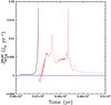 |
Fig. 3 Evolution of the torque on the gainer star |
3.4. Star-disc boundary-layer treatment
Although disc formation in semi-detached binaries is determined by the stellar and orbital properties of the system (Lubow & Shu 1975), we assume the formation of an accretion disc whenever the star reaches its critical spin rate. Our paradigm is that the stellar matter which, cannot be accreted by the fast-rotating and distorted star, will surround the gainer, eventually forming a disc (see Sect. 4.2.2). In practice, the treatment of the boundary layer activates once the star has reached 80% of its critical spin-angular velocity. As a result, the gainer is initially spun up in the same way as if no braking mechanism was present and is then kept at the critical spin-angular velocity when the boundary layer is at work.
Figure 3 shows the evolution of the torque applied on the star due to mass accretion. When the boundary-layer mechanism is activated, the torque quickly drops to zero when the star reaches the critical spin velocity. Since the momentum of inertia of the donor keeps rising due to the increase in mass and radius, angular momentum needs to be evacuated to maintain the rotation at the critical value, hence the temporarily negative value of  (Fig. 2). All the transferred matter is accreted, and the evolution of the system remains conservative.
When a disc forms because the separation is large enough or when the gainer has a small filling-factor, the boundary model is activated, and as long as the gainer’s surface velocity remains below 0.9Ωcrit, the accreted specific angular momentum is basically equal to the Keplerian value of  (38)where R∗ ,eq is the stellar equatorial radius. Note that our computed values for jcrit are in very good agreement with those of Popham & Narayan (1991), who use a different set of equations.
3.5. Evolution of the system
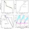 |
Fig. 4 Evolution of our 6 + 3.6 M⊙ system with different braking mechanisms: (solid black line) rotation-free model; (dotted red line) magnetic field 3 kG; (dashed green line) boundary-layer treatment. Top left: mass accretion rate on the gainer. The vertical line represents the epoch when the mass ratio q = 1. Top right: orbital separation. Bottom left: HR diagram for the three configurations: (solid black) rotation-free model; (dotted red) 3 kG magnetic field; (dashed blue) boundary-layer treatment; (dot-dashed green) hotspot (see Appendix A). The open circles correspond to the beginning of mass transfer, triangles to the transition between the rapid and quiescent phase of mass transfer, and squares to the end of mass transfer (only on the rotation-free model). Bottom right: extension of the donor (top cyan hatched area) and gainer (bottom magenta hatched area) within their Roche lobes RL (donor (solid blue lines) gainer (solid red lines)) for the three cases. The y-axis represents the position relative to the system’s centre of mass. The gap between the Roche lobe radii RL of the two stars is because RL is defined as the radius of a sphere with a volume equivalent to the Roche lobe and therefore differs from the true location of the ℒ1 point. |
The evolution of the binary parameters strongly depends on the spin-down mechanism, because it controls how much mass and angular momentum are transferred.
The top right panel of Fig. 4 shows the evolution of the separation for the considered spin-down mechanisms. The “boundary-layer” simulation ends up with a shorter orbital separation (about 100 R⊙, orbital period of 36 days) than the magnetic-field case (about 135 R⊙, orbital period of 59 days), which is slightly less than the canonical “rotation-free” model.
When a boundary layer forms, the star accretes the maximum allowed amount of angular momentum necessary to maintain its rotational velocity at the critical value. This process minimises the angular momentum returned to the orbit, hence leading to a smaller orbital separation compared to the other mechanisms. For the disc-locking mechanism, the gainer’s spin is kept below the critical rate, so more angular momentum is evacuated leading to longer period systems. For the stronger wind-braking mechanism (as compared to disc-locking), more angular momentum will be lost from the system, therefore reducing the orbital separation.
The differences in the mass-transfer rates between the three aforementioned models are small, (see Fig. 4, top left panel) since the separation does not vary between the considered models during the rapid phase of mass transfer. Therefore, the Roche radius – and in turn the mass-transfer rate – of the donor remain unchanged. Then, the differences in the separation are negligible on the (weak) mass-transfer rate during the quiescent phase. As a result, the final masses are exactly the same. The donor star ends up with a mass of 0.8 M⊙ and the gainer at about 8.75 M⊙. The final mass ratios are q = 0.096 for the star-disc spin-down mechanism and q = 0.098 for the wind-braking mechanism.
During the mass-transfer phase, the donor radius equals the Roche radius, which depends on the separation and thus on the braking mechanism. As the Roche radius is smaller for the boundary-layer model than for the magnetic-braking mechanism, so is the donor’s radius (by about 30%; bottom-right panel of Fig. 4).
The bottom-left panel of Fig. 4 presents the Hertzsprung-Russell diagram (HRD) for the same three configurations. There are no differences between these models for the gainer star since roughly the same amount of matter is accreted: the radiative accretor ascends the main sequence at a slightly higher luminosity. On the other hand, the donor’s evolution exhibits small differences during the quiescent mass-transfer phase due to the different evolutionary histories of the separation and stellar radius. By the end of the simulation, all tracks converge to the same point.
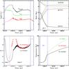 |
Fig. 5 Evolution of our 6 + 3.6 M⊙ system with hotspot formation. Top left: normalised hotspot Lhotspot (solid black line), accretion |

3.6. Hotspot
The hotspot formalism derived in Appendix A provides a self-consistent determination of the β parameter. In this section, it is applied in conjunction with the boundary-layer formalism to avoid super-critical velocities. During the rapid phase, the hotspot luminosity Lhotspot (Fig. 5, top left) is higher than the critical Eddington value  (Eq. (A.15)) and largely exceeds the accretion luminosity
 (39)because of the small impact area (Eq. (A.17)). This hotspot formalism leads to a non-conservative evolution and small values of β during both the rapid and quiescent phases (see bottom-left panel of Fig. 5). While almost the same amount of mass is lost by the donor2 (top-right panel of Fig. 5), the gainer’s final mass is different: 7.4 M⊙ versus 8.8 M⊙ for the fully conservative case. In total, 1.4 M⊙ are expelled from the system, but this barely affects the final mass ratio; 0.1 for the conservative model compared to 0.12 for the hotspot model.
There are two regimes for the evolution of β (see Fig. 5, bottom left). The first one occurs during the onset of mass transfer, when the gainer is still slowly rotating (Ω∗/Ωcrit ≲ 0.2). This phase is characterised by a drop in β as the first term of Eq. (36),  , dominates the second (rotational) term,
  . With increasing velocity, the star enters the second regime where the rotational term, which is proportional to Ω∗, becomes dominant. During this phase, β starts to increase again, because
  gets higher. Eventually, the star reaches its critical spin velocity, and β saturates around 0.6−0.7. The noise in the β profile is due to the explicit dependence of the rotational term on the time-step Δt.
Once the mass ratio has been reversed, the orbital separation starts to increase, leaving space for the formation of an accretion disc. At time t ≈ 5.486 × 10⁷ yr, the stream no longer impacts the star, and our hotspot formalism stops applying, terminating the non-conservative evolution.
In the Hertzsprung-Russell diagram (Fig. 4, bottom-left panel), the gainer is less luminous, because it accretes less mass. For the donor, on the other hand, the presence of a hotspot does not alter its evolution in the HRD. The main effects of this non-conservative evolution are the slight decrease in the final orbital separation (94 R⊙ vs. 100 R⊙ in the conservative case) and a slower acceleration of the gainer’s rotational velocity.
The parameter , defining the hotspot luminosity (Eq. (A.18)), has a strong impact on the critical mass-accretion rate and thus on β. Given the range of values for derived from observations (from  to
to  ; van Rensbergen et al. 2011), a fully conservative or a significantly non-conservative evolution can result from the simulations. In our calculations, varies between 125 and 161, and the total amount of mass ejected is 1.4 M⊙. If we were to use
  , we would have a fully conservative evolution for the same system.
The opacity of the material at the impact location (where the Eddington luminosity is computed) is set to the photospheric value that is higher than the Thomson electron-scattering opacity κes generally used. Given the sensitivity of to this quantity, we ran a simulation using κes for the computation of and found a fully conservative evolution. The opacity has thus a strong impact on β. It is not straightforward (and beyond the scope of this article) to precisely compute the physics (opacity, shock formation) at the impact location, since this depends on the temperature of the disturbed material and the penetration depth of the stream. This depth can be estimated by equating the stream ram pressure ρ | v2 | to the stellar gas pressure (Ulrich & Burger 1976). However, complications arise because the rotation of the star makes the stream impact upon a new undisturbed part of the star at each instant. Moreover, the matter can be ejected directly from the impact location but also from its trail (i.e., from the perturbed material no longer at the impact location) where the opacity may be different.
Due to the large amount of mass transferred in massive short-period binaries, the gainer’s radius may increase until it fills its own Roche radius and the system may then evolve into contact. However, the presence of a hotspot can prevent this evolution, because less mass is accreted onto the gainer star.
In contrast to our simulation, the model of van Rensbergen et al. (2008) for the same system (with initial masses 6 + 3.6 M⊙ and initial period Pinit = 2.5 d) is fully conservative (neglecting winds). It is not straightforward to disentangle the differences between the two runs because of the different approaches used to compute various physical quantities. For instance, the stream velocity is computed in Binstar via ballistic motion, while van Rensbergen et al. (2008) use geometrical arguments. They also use a parametric tidal spin-down prescription, which is more efficient than the one computed in Binstar, derived from the stellar structure. Therefore, the gainer star is more efficiently spun down and, in turn, has a lower mass-loss rate due to the higher (Eq. (A.16)) in their models. The computation of the opacity also differs; we use the photospheric opacity (at τ = 2/3), while they use a parametric expression based on the electron-scattering opacity. For comparison, we implemented their formulation in Binstar and found that less mass is lost from the system (≈0.9 M⊙) mainly, because they neglect the term  in Eq. (36), which is not negligible (
 ) and contributes to a greater decrease
  . As a result, the final separation (bottom-right panel of Fig. 5) also changes between the two hotspot formalisms since it is linked with the masses of the two stars. Our less conservative model leads to a shorter-period system. Nevertheless, both formalisms show the same two phases for the evolution of β.
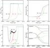 |
Fig. 6 Evolution of our 6 + 3.6 M⊙ system with Pinit = 2.5 days with hotspot and different magnetic field strengths. Black: hotspot with boundary layer (BL) and no magnetic field. Red: hotspot (no BL) + magnetic field | B∗ | = 1 kG. Green: hotspot (no BL) + magnetic field | B∗ | = 2 kG. The red simulation stops when the gainer reaches its critical spin-angular momentum (indicated by a red circle). Top left: surface spin-angular velocity. Top right: orbital separation. Bottom left: accretion efficiency β. Bottom right: masses. |
3.7. Hotspot and magnetic braking
We mentioned that β is a key parameter for the magnetic-wind braking. In Sect. 3.2, only stellar winds have been considered as a mass-loss mechanism from the system, but the matter emanating from the hotspot might contribute to the magnetic-wind braking by increasing the mass-loss rate ṀW in Eq. (8). As a result, a lower magnetic-field strength is needed to keep the gainer’s spin velocity below the critical value.
In the configuration with a hotspot plus a 1 kG magnetic field and no boundary-layer mechanism, the gainer reaches the critical rate, although later than in the conservative case (Fig. 6). Above 2 kG, the critical rotation can be avoided but the required field strength still remains higher than measured in Algols.
As expected, coupling the expelled material to the magnetic field will increase the system angular momentum loss and thus the separation. As a consequence, the impact velocity will be greater and according to Eq. (36), the threshold for mass ejection will be lower. As explained previously, the value of β drops until the rotational term  starts to dominate. The β profiles diverge more as time goes on because of the increasing difference in the gainer’s luminosities due to their different masses. In the case of a strong magnetic field (2 kG), β drops to lower values (β ≈ 0.1) and for a much longer duration. The donor reaches the same final mass (Md ≈ 0.8 M⊙), but the final mass ratio increases significantly from 0.1 to 0.25 because 3.6 M⊙ are removed from the system.
In their study, Dervişoğlu et al. (2010) use a constant value of β ranging from 0.1 to 0.9 to account for the system mass-loss. This is in contrast to our approach where β is computed consistently. Our simulations cannot maintain values as low as those used by these authors during the entire phase of mass transfer and this explains why in our case the magnetic-wind braking is not as efficient. Because of our poor knowledge of the hotspot outflow geometry and its link with the magnetic field, that coupling should be regarded as exploratory.
4. Can observations help constraining Algol evolution?
4.1. Predicting the mass ejected from the hotspot
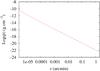 |
Fig. 7 Density profile of the matter expelled by the hotspot and surrounding the system. The x-axis represents the angular extent for a system located at 100 pc. The profile starts at the stellar radius of the gainer (R∗ = 2.2 × 1011 cm) and is cut at 2 arcmin. The density drops below the mean density of the ISM value at 12 arcmin (1.05 × 1018 cm) from the star. |
It is not clear what happens to the matter ejected via the hotspot, whether it freely escapes the system as assumed in our simulation or if it remains in the gainer’s Roche lobe to be eventually re-accreted. Since the hotspot luminosity exceeds the Eddington luminosity in our model, we expect the matter to reach the escape velocity  (40)where Meff is the effective gravitational mass felt by the wind (Castor et al. 1975):
  (41)where κes is the Thomson electron-scattering opacity. In this equation, the luminosity LΣ is due to both the star and the hotspot. We further assume that the flow, once ejected, is accelerated by radiation pressure. Following Castor et al. (1975)’s prescription for radiation-driven winds, the material velocity at a distance r from the gainer is then given by
  (42)where α is a force multiplier parameter (Lamers & Cassinelli 1999) that has been set to three different values: α = 0.465 (for TΣ = 6 × 10³ K3); α = 0.5 (for TΣ = 3 × 10⁴ K typical of hotspot temperatures; van Rensbergen et al. 2010b); and α = 0.640 (for TΣ = 5 × 10⁴ K). For the sake of simplicity, the influence of the secondary star and the internal energy of the flow have been neglected.
The density of the material surrounding the system at a given time t and distance r is calculated using the continuity equation  (43)where
  is a solid angle over which the material is ejected. The geometry of the mass ejection is badly constrained but will probably be collimated due to the small area of the hotspot. For simplicity, we use
  . The mass flow Ṁflow(r,t) at time t and position r is equal to the system mass-loss rate
  estimated at the time such that
  . In other words, r is the distance travelled by the ejected layer, since the beginning of the non-conservative phase.
In this simplistic model, it is also possible to follow the chemical stratification of the expelled material because we know from the stellar model the composition of the ejected layers at each time-step. The chemical changes are small until the gainer’s mass has dropped below ≈3 M⊙, and the CNO-processed layers start to be ejected. By the end of the non-conservative evolution, the abundance of 14N has increased by a factor of 5, while 12C has been almost completely depleted. Since C+N+O remains constant, the global metallicity of the ejected material is almost constant.
The final density profile (when the non-conservative phase ends) is shown in Fig. 7. The x-axis represents the angle subtended by the flow for a system located at 100 pc (to fix the ideas, we remind that β Persei is situated at ≈30 pc and β Lyræ at ≈300 pc). The density drops below the mean interstellar medium (ISM) density (≈10-24 g cm-3, Ferrière 2001)4 at 12 arcmin from the star, or at 1.05 × 1018 cm. Closer to the star, the density rises up to 10-9 g cm-3 in the thin region of the wind acceleration. Finally, we report that the parameter α has almost no impact on the density profile in the inner region (inside the 2 arcmin region).
The calculation of the radiative transfer through this surrounding material would allow a meaningful comparison with infrared flux observations, but it is beyond the scope of this article and deferred to a future work.
4.2. Observational constraints on the spin-down mechanism
In this section, we attempt to identify observational constraints that can corroborate or invalidate spin-down mechanisms and non-conservative evolution.
4.2.1. Classification of Algol systems
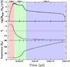 |
Fig. 8 Evolution of the mass-transfer rate (top-panel), mass ratio (q = Md/Mg), and separation for our 6 + 3.6 M⊙ system with Pinit = 2.5 days. The different evolutionary states are coloured in red (Class I), green (Class II), and blue (Class III). |
Depending on their observable properties (presence of a disc, mass ratio, and mass-transfer rate, etc.), binary systems in a given and the same evolutionary state from a theoretical standpoint may end up being associated with different observational classes. Therefore, we define theoretical classes based on our simulation results and associate a prototype with each class to ease the comparison between observations and models.
The first class (Class I, see Fig. 8) refers to the state before the mass-ratio reversal when the mass ratio and the orbital period decrease. Observational prototypes are UX Mon (Sudar et al. 2011) or SV Cen (see Table 2). During this phase, mass transfer is increasing until the system enters the rapid mass-transfer phase. These objects can host accretion discs and exhibit bipolar jet and/or show strong UV emission lines likely due to the formation of a hotspot (Guinan 1989). Taranova & Shenavrin (1997) also report excess IR emission attributed to dusty material surrounding the system.
For Class II (Fig. 8), the mass ratio is reversed and the mass-transfer rate is at a maximum. This stage is the realm of β Lyræ or W Ser objects (see Table 2). The same features as for Class I objects (discs, jets, hotspots, and circumbinary gas) may possibly be present, but Class II objects differ from Class I by their longer and increasing orbital periods. They are often referred as “active” or “hyper-active” Algols.
The last class (Class III, Fig. 8) includes quiescent objects with their mass ratio reversed. It is during this phase that the separation evolves the most, but the mass ratio remains roughly constant. This class mainly corresponds to genuine Algol systems (including the prototype β Per; see Table 2).
4.2.2. Observational constraints from Class I-II objects
Spin-down mechanisms and system-mass loss may act more efficiently during these phases (Classes I-II) and lead to clearer observational signatures, making these systems more interesting despite that they do not last long compared to Class III objects.
The observationally defined W Ser systems that we associate in our theoretical system to Class I-II objects were first detected and classified owing to their UV emission, which is attributed to the impact of the accretion stream on the edge of the accretion disc. The presence of gas around these systems (see Sect. 4.2.1) is consistent with mass ejection from a hotspot.
Accretion discs are frequently detected in Class I-II systems (Guinan 1989; van Rensbergen et al. 2011) and contribute to the regulation of the gainer’s spin velocity. The Doppler tomography method (mapping the circumstellar matter in a system) has been extensively applied to β Lyræ systems (Richards et al. 1995; Albright & Richards 1996; Richards 2004; Miller et al. 2007; Richards et al. 2010). These studies reveal the presence of disc-like structures, even in the case where the gainer has a large filling factor and where direct impact is expected instead (Barai et al. 2004). This supports our paradigm of disc formation around critically-rotating gainers and the activation of the boundary-layer mechanism (Sect. 2.4) or the disc-locking mechanism (Sect. 2.2.2), especially for Class I-II objects where the separation is short and the mass-transfer rate high.
4.3. On the rotation of Algols
Most observed Algol systems have an accretor with a rotational velocity in the range 0.1 < Ω∗/ΩKep < 0.4 (van Hamme & Wilson 1990), but some of them are very rapidly rotating with a Keplerian (or close to Keplerian) surface spin velocity (McNamara 1957; Hansen & McNamara 1959; Wilson 1989; Mukherjee et al. 1996). Unfortunately, there are no observations of spin rates for the gainer in the interesting W Ser objects, because they are completely embedded in their accretion discs. The very high spin velocities in genuine Algols can be regarded as the signature of recent angular-momentum transfer or as evidence of the braking mechanism that did not have the time to yet operate. This is consistent with the boundary-layer paradigm that necessarily leads the star to critical rotation. On the other hand, another mechanism must be advocated to spin the gainer down after the rapid phase of mass transfer to explain the slow rotators. This can be due to tides or magnetic braking (with a low magnetic field strength <3 kG), which are processes that were inefficient during the earlier evolution of rapid mass transfer.
If the star is not rotating as a solid body, the outermost layers will first be spun up and, because of the differential rotation, instabilities will develop and allow angular momentum to be transported in the interior. In this case, the outermost layers will be accelerated to the critical velocity after a low amount of mass has been accreted, and we may expect the boundary-layer mechanism to be activated earlier during the evolution. If the angular-momentum redistribution inside the star is not efficient enough for the gainer to reach solid-body rotation by the end of the mass-transfer phase, less angular momentum will then be stored into the star and a larger amount given back to the orbit, thus increasing the orbital separation.
However, rotation can also affect the mechanical and thermal structure of the star, because it brakes the spherical symmetry. Considering these effects in the stellar structure equations (Endal & Sofia 1976, hereafter referred to as centrifugally supported models) leads to larger effective radii and cooler surface temperatures. Because of the short separation, the result is that our system runs into contact just before the reversal of the mass ratio. However, this contact phase can be avoided if the initial period is increased to ≈5 days (instead of 2.5 days). To reproduce the evolution of canonical models, for which the effects of departure from spherical symmetry are not accounted, our centrifugally supported models must start with a longer initial period. It also implies that neglecting these structural effects of rotation will produce less contact systems. Finally, we also point out that less room is left for an accretion disc to form due to the growth of the stellar equatorial radius, and mass loss through the third Lagrangian point ℒ3 may be enhanced due to the growth of the stellar equatorial radius.
Finally, rotational instabilities also contribute to the transport of chemicals, and the mixing is likely to be very efficient in the gainer star because of the strong torques applied at the surface (Decressin et al. 2009). Similar to fast rotating massive stars, we may expect the accretor to evolve almost chemically homogeneously (Maeder 1987; de Mink et al. 2010), showing surface enhancements in helium and nitrogen. These alterations of the surface composition can decrease the envelope opacity, making the gainer star more compact and more luminous, thus counterbalancing the radius growth associated with the rotational deformation of the structure described above. Clearly, stellar calculations, including angular momentum transport and rotationally induced mixing, are required to clarify the situation.
5. Conclusions
In this study, we performed the first binary-evolution calculations that consistently consider the torques arising from magnetic fields and star-disc interaction. This is the first attempt to confront several braking mechanisms with the use of the state-of-the-art binary-star evolutionary code Binstar. We show that the torques due to magnetic field and star-disc interaction can prevent the accreting star from reaching a super-critical velocity, although the magnetic-field strength required are stronger than that of typical Algols. Tides are shown to be inefficient, but we do not exclude them to slow down the gainer after the mass-transfer phase. We show that some orbital key parameters of the system (e.g. the orbital separation) strongly depend on the spin-down mechanism.
Our new hotspot prescription leads to a less conservative evolution than the van Rensbergen et al. (2008) formalism. We showed that the opacity of the impacted material and the geometry of the accretion (through the parameter) are two highly-sensitive, badly-constrained key parameters for the computation of non-conservative models, stressing the need for observations and/or hydrodynamic simulations of hotspots.
A better understanding of disc formation around critically-rotating accretors and observational constraints on the magnetic-field strength of these stars are needed. In the future, we wish to establish a grid of non-conservative evolutions using Binstar to perform a statistical study, comparing these data to observational data and evaluate the impact of the various spin-down mechanisms and the hotspot formalism on the properties of the binary remnant.
A criterion that defines whether a system is in the direct impact or disc accretion regime and is based on the binary parameters (mass ratio and orbital separation).
Changes in the mass-accretion rate affect the mass-loss rate of the donor star, because the modification of the mass ratio impacts on the Roche radius.
TΣ is the equivalent temperature of the hotspot plus the star, obtained by summing the fluxes and applying Stefan-Boltzmann’s law.
In principle, it is the equilibrium between the ram pressures of the wind and of the ISM that imposes the boundary of the stellar flow. However, that boundary is even further away than the one based on the density used here since the hotspot stream velocity is much larger than the ISM velocity – a few tens of km s-1 at most.
Hence, the term “accretion luminosity” for the quantity expressed by Eq. (A.12) is not especially well suited! Unfortunately, it is accepted terminology.
Acknowledgments
We are most grateful to Walter van Rensbergen and Jean-Pierre de Grève for sharing their great expertise and for many fruitful discussions. R.D. and P.J.D. acknowledge support from the Communauté française de Belgique – Actions de Recherche Concertées. LS is an FNRS Researcher. P.J.D. is Chargé de Recherche (FNRS-F.R.S.).
References
- Ak, H., Chadima, P., Harmanec, P., et al. 2007, A&A, 463, 233 [NASA ADS] [CrossRef] [EDP Sciences] [Google Scholar]
- Albright, G. E., & Richards, M. T. 1996, ApJ, 459, L99 [NASA ADS] [CrossRef] [Google Scholar]
- Armitage, P. J., & Clarke, C. J. 1996, MNRAS, 280, 458 [NASA ADS] [Google Scholar]
- Barai, P., Gies, D. R., Choi, E., et al. 2004, ApJ, 608, 989 [NASA ADS] [CrossRef] [Google Scholar]
- Bisnovatyi-Kogan, G. S. 1993, A&A, 274, 796 [NASA ADS] [Google Scholar]
- Bondi, H., & Hoyle, F. 1944, MNRAS, 104, 273 [NASA ADS] [CrossRef] [Google Scholar]
- Budding, E., Erdem, A., Çiçek, C., et al. 2004, A&A, 417, 263 [NASA ADS] [CrossRef] [EDP Sciences] [Google Scholar]
- Bychkov, V. D., Bychkova, L. V., & Madej, J. 2003, A&A, 407, 631 [NASA ADS] [CrossRef] [EDP Sciences] [Google Scholar]
- Bychkov, V. D., Bychkova, L. V., & Madej, J. 2009, MNRAS, 394, 1338 [Google Scholar]
- Capper, S., Cash, J., & Mazzia, F. 2007, Int. J. Comput. Sci. Math., 1, 42 [CrossRef] [Google Scholar]
- Castor, J. I., Abbott, D. C., & Klein, R. I. 1975, ApJ, 195, 157 [NASA ADS] [CrossRef] [Google Scholar]
- Chandrasekhar, S. 1939, An introduction to the study of stellar structure (Chicago: University of chigaco press), 55, 142 [NASA ADS] [Google Scholar]
- Colpi, M., Nannurelli, M., & Calvani, M. 1991, MNRAS, 253, 55 [NASA ADS] [Google Scholar]
- de Greve, J. P. 1993, A&AS, 97, 527 [NASA ADS] [Google Scholar]
- de Mink, S. E., Pols, O. R., & Glebbeek, E. 2007, in Unsolved Problems in Stellar Physics: A Conference in Honor of Douglas Gough, eds. R. J. Stancliffe, G. Houdek, R. G. Martin, & C. A. Tout, AIP Conf. Ser., 948, 321 [Google Scholar]
- de Mink, S. E., Cantiello, M., Langer, N., & Pols, O. R. 2010, in AIP Conf. Ser. 1314, eds. V. Kologera, & M. van der Sluys, 291 [Google Scholar]
- Decressin, T., Mathis, S., Palacios, A., et al. 2009, A&A, 495, 271 [NASA ADS] [CrossRef] [EDP Sciences] [Google Scholar]
- Dermine, T., Jorissen, A., Siess, L., & Frankowski, A. 2009, A&A, 507, 891 [NASA ADS] [CrossRef] [EDP Sciences] [Google Scholar]
- Dervişoğlu, A., Tout, C. A., & Ibanoğlu, C. 2010, MNRAS, 406, 1071 [NASA ADS] [Google Scholar]
- Eggleton, P. P. 2000, New A Rev., 44, 111 [Google Scholar]
- Eggleton, P. P., & Kiseleva-Eggleton, L. 2002, ApJ, 575, 461 [NASA ADS] [CrossRef] [Google Scholar]
- Endal, A. S., & Sofia, S. 1976, ApJ, 210, 184 [NASA ADS] [CrossRef] [Google Scholar]
- Ferrière, K. M. 2001, Rev. Mod. Phys., 73, 1031 [NASA ADS] [CrossRef] [Google Scholar]
- Flannery, B. P. 1975, MNRAS, 170, 325 [NASA ADS] [CrossRef] [Google Scholar]
- Ghosh, P., & Lamb, F. K. 1979, ApJ, 232, 259 [NASA ADS] [CrossRef] [Google Scholar]
- Giannuzzi, M. A. 1981, A&A, 103, 111 [NASA ADS] [Google Scholar]
- Giuricin, G., Mardirossian, F., & Mezzetti, M. 1983, ApJS, 52, 35 [NASA ADS] [CrossRef] [Google Scholar]
- Guinan, E. F. 1989, Space Sci. Rev., 50, 35 [NASA ADS] [CrossRef] [Google Scholar]
- Hansen, K., & McNamara, D. H. 1959, ApJ, 130, 791 [NASA ADS] [CrossRef] [Google Scholar]
- Huang, S.-S. 1963, ApJ, 138, 481 [NASA ADS] [CrossRef] [Google Scholar]
- Hubrig, S., North, P., Schöller, M., & Mathys, G. 2006, Astron. Nachr., 327, 289 [NASA ADS] [CrossRef] [Google Scholar]
- Hubrig, S., North, P., & Schöller, M. 2007, Astron. Nachr., 328, 475 [NASA ADS] [CrossRef] [Google Scholar]
- Ichikawa, S., & Osaki, Y. 1994, PASJ, 46, 621 [NASA ADS] [Google Scholar]
- Kippenhahn, R., & Weigert, A. 1990, Stellar Structure and Evolution (New york: Springer-Verlag), Astron. Astrophys. Lib., 468 [Google Scholar]
- Kolb, U., & Ritter, H. 1990, A&A, 236, 385 [NASA ADS] [Google Scholar]
- Kopal, Z. 1955, Ann. Astrophys., 18, 379 [Google Scholar]
- Kruszewski, A. 1964, Acta Astron., 14, 231 [NASA ADS] [Google Scholar]
- Kruszewski, A. 1967, Acta Astron., 17, 297 [NASA ADS] [Google Scholar]
- Lamers, H. J. G. L. M., & Cassinelli, J. P. 1999, Introduction to Stellar Winds (Cambridge: Cambridge University press), 26, 171 [Google Scholar]
- Lamers, H. J. G. L. M., Snow, T. P., & Lindholm, D. M. 1995, ApJ, 455, 269 [NASA ADS] [CrossRef] [Google Scholar]
- Lin, D. N. C., & Papaloizou, J. 1979, MNRAS, 186, 799 [NASA ADS] [CrossRef] [Google Scholar]
- Livio, M., & Pringle, J. E. 1992, MNRAS, 259, 23P [NASA ADS] [CrossRef] [Google Scholar]
- Lomax, J. R., Hoffman, J. L., Elias, II, N. M., Bastien, F. A., & Holenstein, B. D. 2012, ApJ, 750, 59 [CrossRef] [Google Scholar]
- Lubow, S. H., & Shu, F. H. 1975, ApJ, 198, 383 [NASA ADS] [CrossRef] [Google Scholar]
- Maeder, A. 1987, A&A, 178, 159 [NASA ADS] [Google Scholar]
- Maeder, A. 2009, Physics, Formation and Evolution of Rotating Stars, (Berlin, Heidelberg: Springer), Astron. Astrophys. Lib. [Google Scholar]
- Maeder, A., & Meynet, G. 2001, A&A, 373, 555 [NASA ADS] [CrossRef] [EDP Sciences] [Google Scholar]
- Massevitch, A., & Yungelson, L. 1975, Mem. Soc. Astron. Ital., 46, 217 [Google Scholar]
- McNamara, D. H. 1957, PASP, 69, 574 [NASA ADS] [CrossRef] [Google Scholar]
- Mestel, L. 1968, MNRAS, 138, 359 [NASA ADS] [CrossRef] [Google Scholar]
- Mezzetti, M., Giuricin, G., & Mardirossian, F. 1980, A&A, 83, 217 [NASA ADS] [Google Scholar]
- Miller, B., Budaj, J., Richards, M., Koubský, P., & Peters, G. J. 2007, ApJ, 656, 1075 [NASA ADS] [CrossRef] [Google Scholar]
- Mukherjee, J., Peters, G. J., & Wilson, R. E. 1996, MNRAS, 283, 613 [NASA ADS] [CrossRef] [Google Scholar]
- Nelson, C. A., & Eggleton, P. P. 2001, ApJ, 552, 664 [NASA ADS] [CrossRef] [Google Scholar]
- Packet, W. 1981, A&A, 102, 17 [NASA ADS] [Google Scholar]
- Paczynski, B. 1991, ApJ, 370, 597 [NASA ADS] [CrossRef] [Google Scholar]
- Padmanabhan, P. 2000, Theoretical astrophysics. Astrophysical processes (Cambridge: Cambridge University press), 1 [Google Scholar]
- Peters, G. J., & Polidan, R. S. 2004, Astron. Nachr., 325, 225 [Google Scholar]
- Piddington, J. H. 1983, Ap&SS, 90, 217 [NASA ADS] [CrossRef] [Google Scholar]
- Piirola, V., Berdyugin, A., Mikkola, S., & Coyne, G. V. 2005, ApJ, 632, 576 [NASA ADS] [CrossRef] [Google Scholar]
- Popham, R., & Narayan, R. 1991, ApJ, 370, 604 [NASA ADS] [CrossRef] [Google Scholar]
- Press, W. H., Teukolsky, S. A., Vetterling, W. T., & Flannery, B. P. 2007, Numerical Recipes 3rd edn. The Art of Scientific Computing (New York, USA: Cambridge University Press) [Google Scholar]
- Pringle, J. E. 1981, ARA&A, 19, 137 [NASA ADS] [CrossRef] [Google Scholar]
- Refsdal, S., Roth, M. L., & Weigert, A. 1974, A&A, 36, 113 [NASA ADS] [Google Scholar]
- Reimers, D. 1975, Circumstellar envelopes and mass loss of red giant stars (New York: Springer-Verlag), 229 [Google Scholar]
- Retter, A., Richards, M. T., & Wu, K. 2005, ApJ, 621, 417 [NASA ADS] [CrossRef] [Google Scholar]
- Richards, M. T. 2004, Astron. Nachr., 325, 229 [NASA ADS] [CrossRef] [Google Scholar]
- Richards, M. T., Albright, G. E., & Bowles, L. M. 1995, ApJ, 438, L103 [NASA ADS] [CrossRef] [Google Scholar]
- Richards, M. T., Sharova, O. I., & Agafonov, M. I. 2010, ApJ, 720, 996 [NASA ADS] [CrossRef] [Google Scholar]
- Ritter, H. 1988, A&A, 202, 93 [NASA ADS] [Google Scholar]
- Sarna, M. J. 1993, MNRAS, 262, 534 [NASA ADS] [CrossRef] [Google Scholar]
- Sarna, M. J., Yerli, S. K., & Muslimov, A. G. 1998, MNRAS, 297, 760 [NASA ADS] [CrossRef] [Google Scholar]
- Shakura, N. I., & Sunyaev, R. A. 1973, A&A, 24, 337 [NASA ADS] [Google Scholar]
- Siess, L. 2006, A&A, 448, 717 [NASA ADS] [CrossRef] [EDP Sciences] [Google Scholar]
- Siess, L., Izzard, R. G., Davis, P. J., & Deschamps, R. 2013, A&A, 550, A100 [NASA ADS] [CrossRef] [EDP Sciences] [Google Scholar]
- Spruit, H. C. 1999, A&A, 349, 189 [NASA ADS] [Google Scholar]
- Stȩpień, K. 2000, A&A, 353, 227 [NASA ADS] [Google Scholar]
- Sudar, D., Harmanec, P., Lehmann, H., et al. 2011, A&A, 528, A146 [NASA ADS] [CrossRef] [EDP Sciences] [Google Scholar]
- Sytov, A. Y., Kaigorodov, P. V., Bisikalo, D. V., Kuznetsov, O. A., & Boyarchuk, A. A. 2007, Astron. Rep., 51, 836 [Google Scholar]
- Taranova, O. G., & Shenavrin, V. I. 1997, Astron. Lett., 23, 698 [NASA ADS] [Google Scholar]
- Tout, C. A., & Pringle, J. E. 1992, MNRAS, 256, 269 [NASA ADS] [Google Scholar]
- Ulrich, R. K., & Burger, H. L. 1976, ApJ, 206, 509 [NASA ADS] [CrossRef] [Google Scholar]
- van Hamme, W., & Wilson, R. E. 1990, AJ, 100, 1981 [Google Scholar]
- van Rensbergen, W., de Greve, J. P., de Loore, C., & Mennekens, N. 2008, A&A, 487, 1129 [NASA ADS] [CrossRef] [EDP Sciences] [Google Scholar]
- van Rensbergen, W., de Greve, J.-P., Mennekens, N., de Loore, B., & Jansen, K. 2010a, in AIP Conf. Ser. 1314, eds. V. Kologera, & M. van der Sluys, 45 [Google Scholar]
- van Rensbergen, W., de Greve, J. P., Mennekens, N., Jansen, K., & de Loore, C. 2010b, A&A, 510, A13 [NASA ADS] [CrossRef] [EDP Sciences] [Google Scholar]
- van Rensbergen, W., de Greve, J. P., Mennekens, N., Jansen, K., & de Loore, C. 2011, A&A, 528, A16 [NASA ADS] [CrossRef] [EDP Sciences] [Google Scholar]
- Weber, E. J., & Davis, Jr., L. 1967, ApJ, 148, 217 [NASA ADS] [CrossRef] [Google Scholar]
- Whitehurst, R. 1988, MNRAS, 232, 35 [NASA ADS] [Google Scholar]
- Wilson, R. E. 1989, Space Sci. Rev., 50, 191 [NASA ADS] [CrossRef] [Google Scholar]
- Wilson, R. E., & Starr, T. C. 1976, MNRAS, 176, 625 [NASA ADS] [CrossRef] [Google Scholar]
- Zahn, J.-P. 1977, A&A, 57, 383 [NASA ADS] [Google Scholar]
- Zahn, J.-P. 1989, A&A, 220, 112 [NASA ADS] [Google Scholar]
Appendix A: Hotspots and critical mass-transfer rate
In this Appendix, we derive a limit for the gainer’s mass-accretion rate by imposing that the luminosity at the hotspot location always remains below the critical Eddington value (Eq. (35)). In the case of direct impact, the kinetic energy of the gas stream emerging from the inner Lagrangian point ℒ1 is partly converted into thermal energy causing a hotspot and is partly radiated away.
To calculate the accretion luminosity (Lacc), we estimate the Jacobi constant (only conserved quantity in our problem) of a test particle at ℒ1. In the rotating frame, 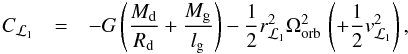 (A.1)where lg is the distance between the centre of the gainer and ℒ1; rℒ1 is the distance between ℒ1 and the centre of mass of the system; vℒ1 is the initial speed of the stream at ℒ1 in the rotating frame; and Rd is the radius of the donor filling its Roche lobe. The last term is usually negligible because, the velocity of the particle at ℒ1 (assumed to be equal to the sound speed) is much lower than the orbital velocity (vℒ1 ≪ rℒ1Ωorb). Similarly, we define Cimp at the impact location:
 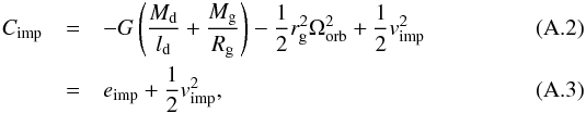 where ld is the distance between the centre of the donor and the hotspot; vimp is the stream velocity in the rotating frame at the impact location; and rg is the distance between the centre of mass of the system and the hotspot. Since Cℒ1 = Cimp, the energy gained by the stream is written as
 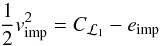 (A.4)and is partially radiated away by the hotspot and imparted to the star in the form of internal energy. Note that the stream velocity at impact vimp is consistently computed by following the ballistic motion of the stream (see Sect. 2.5) in the rotating frame in Binstar. Before the accretion starts, the gainer’s total energy (in the rotating frame, e.g. Padmanabhan 2000) is given by
 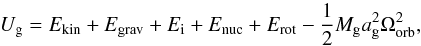 (A.5)where ag is the distance between the centre of mass of the system and the centre of mass of the gainer. After the mass deposition,
 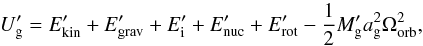 (A.6)where
  and Ekin are the rotational and radial motion kinetic energy of the star, and Egrav, Ei, and Enuc are the gravitational, internal, and nuclear energy content of the star, respectively (Kippenhahn & Weigert 1990). Conservation of the total energy of the system composed of the gainer and accreted material (we neglect changes in the donor’s energy) is written as
 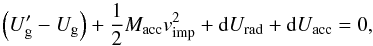 (A.7)where Macc = Ṁacc × Δt is the accreted mass; dUrad is the energy radiated away by the star; and dUacc the energy lost (by radiation) during the accretion process. For a star in hydrostatic equilibrium, we have
 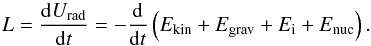 (A.8)In the latter expression, we did not consider the rotational kinetic energy, because it is not accounted for in the stellar structure equations (there is no feed back of rotation on the star’s structure). Inserting Eqs. (A.4)−(A.6) into (A.7) with the help of (A.8) we obtain
 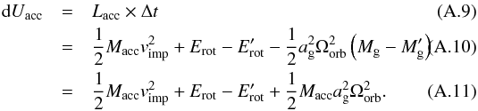 In a binary system with rotating stars, the accretion luminosity is finally written as
 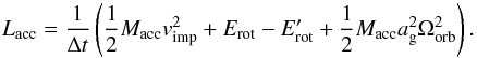 (A.12)Considering that not all the accretion luminosity is radiated away5 (since some fraction is used to increase the internal energy), we introduce the factor αacc < 1 to evaluate the actual luminosity associated with accretion:
  (A.13)
The matter at the hotspot location will be ejected if the hotspot luminosity is higher than the gainer’s Eddington luminosity Ledd,g:  (A.14)where κ is the plasma opacity. However, there are a few subtleties to handle properly. First, we should use the Eddington luminosity corrected for the effects of stellar rotation (Maeder 2009) for rotating stars
 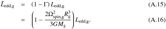 Second, the stellar luminosity contributes to the accretion luminosity in powering the mass ejection from the hotspot. However, the surfaces involved are different, and this must be considered, especially in the comparison to the Eddington luminosity, whose 4π factor in expression Eq. (A.14) implicitly assumes that the whole sphere contributes to the luminosity. For the purpose of this comparison, it is therefore necessary to multiply Lacc,rad by the factor Sstar/Shotspot to make all luminosities correspond to the same surface:
 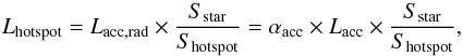 (A.17)or in other words
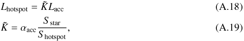 where Shotspot and Sstar are the hotspot and gainer’s surface areas, respectively. Values of have been calibrated by van Rensbergen et al. (2011), and we use their model
 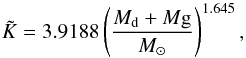 (A.20)which only depends on the total mass of the system. Thus, matter at the hotspot location will be ejected if
  (A.21)where is the gainer’s Eddington luminosity and Lg is its luminosity.
The critical rate above which the hotspot luminosity prevents matter from being accreted is given by solving for Ṁacc in Eq. (A.12) combined with Eqs. (A.18), (A.21), and (A.13), which then yields (Eq. (36)) 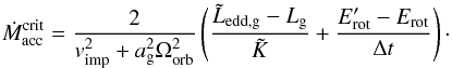 (A.22)When the mass-transfer rate exceeds the critical value, no mass can be accreted.
van Rensbergen et al. (2008) derived a different expression for (their Eq. (18)), which is written using our notations as ![Mathematical equation: \appendix \setcounter{section}{1} \begin{equation} \dot{M}_{\mathrm{acc}}^{\mathrm{crit}} = \frac{2}{v_{\mathrm{imp}}^{2}} \left[ \left( \Delta E \frac{R_{\mathrm{g}}L_{\mathrm{edd},g}}{G M_{\mathrm{g}}} - L_{\mathrm{g}} \right) \frac{1}{\tilde{K}} + \frac{E_{\mathrm{rot}}^{\prime} - E_{\mathrm{rot}}}{\Delta t} \right] ,\label{eq:VUB_macc} \end{equation}](/articles/aa/full_html/2013/09/aa21509-13/aa21509-13-eq293.png) (A.23)where
(A.23)where  Based on our simulations of a 6 + 3.6 M⊙ system with initial period Pinit = 2.5 days, we find that Egrav ≈ 2 − 3 × | Eeq | ≫ Eorb which allows us to simplify Eq. (A.23) (neglecting the Erot terms)
 ![Mathematical equation: \appendix \setcounter{section}{1} \begin{eqnarray} \dot{M}_{\mathrm{acc}}^{\mathrm{crit}} & \approx & \frac{2}{v_{\mathrm{imp}}^{2}\tilde{K}} \left[ \left( 1 + \frac{E_{\mathrm{eq}}}{E_{\mathrm{pot}}} \right) L_{\mathrm{edd,g}} - L_{\mathrm{g}} \right]\\ & \approx & \ \frac{2}{v_{\mathrm{imp}}^{2} \tilde{K} } \left[ \left( 1 - \frac{ \Omega_{\mathrm{spin,g}}^{2} R_{\mathrm{g}}^{3} } { 2 G M_{\mathrm{g}}} \right) L_{\mathrm{edd,g}} - L_{\mathrm{g}} \right] \\ & \approx & {\frac{2}{v_{\mathrm{imp}}^{2}\tilde{K} } } \left( \breve{L}_{\mathrm{edd,g}} - L_{\mathrm{g}} \right) . \end{eqnarray}](/articles/aa/full_html/2013/09/aa21509-13/aa21509-13-eq297.png) This formulation is very comparable to our Eq. (36) in the case that Erot is small, apart from some numerical factors of order of unity and the presence of in our formalism.
This formulation is very comparable to our Eq. (36) in the case that Erot is small, apart from some numerical factors of order of unity and the presence of in our formalism.
All Tables
Summary of the angular-momentum transfer rates involved in a non-conservative system (β < 1).
All Figures
|
Fig. 1 Evolution of the mass-transfer rate (top), stellar masses (middle), surface velocity (bottom) for a 6 M⊙ donor (solid black line), and 3.6 M⊙ gainer (dotted red line) system with initial period Pinit = 2.5 days. |
| In the text | |
|
Fig. 2 Evolution of the gainer’s surface velocity (normalised to the critical velocity) for different spin-down mechanisms for our 6 + 3.6 M⊙ system with an initial period Pinit = 2.5 days. The horizontal line represents the critical spin-angular rotation of the star. All simulations are stopped when Ωsurf ≈ Ωcrit. Top panel: solid black line (labelled “Ref.”): | B∗ | = 0 kG, no braking mechanism; dotted red line (labelled “B.-L.”): boundary-layer mechanism, no magnetic field; dashed green line: Zahn (1989) tidal effect treatment only; long-dashed blue line: magnetic braking with | B∗ | = 3 kG. Bottom panel: solid black line: magnetic braking with | B∗ | = 1 kG; dotted red line: magnetic braking with | B∗ | = 2 kG; dashed green line (labelled M.-W.): magnetic-wind braking only with | B∗ | = 3 kG; long-dashed blue line (labelled D.-L.): disc locking only with | B∗ | = 3 kG. |
| In the text | |
|
Fig. 3 Evolution of the torque on the gainer star |
| In the text | |
|
Fig. 4 Evolution of our 6 + 3.6 M⊙ system with different braking mechanisms: (solid black line) rotation-free model; (dotted red line) magnetic field 3 kG; (dashed green line) boundary-layer treatment. Top left: mass accretion rate on the gainer. The vertical line represents the epoch when the mass ratio q = 1. Top right: orbital separation. Bottom left: HR diagram for the three configurations: (solid black) rotation-free model; (dotted red) 3 kG magnetic field; (dashed blue) boundary-layer treatment; (dot-dashed green) hotspot (see Appendix A). The open circles correspond to the beginning of mass transfer, triangles to the transition between the rapid and quiescent phase of mass transfer, and squares to the end of mass transfer (only on the rotation-free model). Bottom right: extension of the donor (top cyan hatched area) and gainer (bottom magenta hatched area) within their Roche lobes RL (donor (solid blue lines) gainer (solid red lines)) for the three cases. The y-axis represents the position relative to the system’s centre of mass. The gap between the Roche lobe radii RL of the two stars is because RL is defined as the radius of a sphere with a volume equivalent to the Roche lobe and therefore differs from the true location of the ℒ1 point. |
| In the text | |
|
Fig. 5 Evolution of our 6 + 3.6 M⊙ system with hotspot formation. Top left: normalised hotspot Lhotspot (solid black line), accretion |
| In the text | |
|
Fig. 6 Evolution of our 6 + 3.6 M⊙ system with Pinit = 2.5 days with hotspot and different magnetic field strengths. Black: hotspot with boundary layer (BL) and no magnetic field. Red: hotspot (no BL) + magnetic field | B∗ | = 1 kG. Green: hotspot (no BL) + magnetic field | B∗ | = 2 kG. The red simulation stops when the gainer reaches its critical spin-angular momentum (indicated by a red circle). Top left: surface spin-angular velocity. Top right: orbital separation. Bottom left: accretion efficiency β. Bottom right: masses. |
| In the text | |
|
Fig. 7 Density profile of the matter expelled by the hotspot and surrounding the system. The x-axis represents the angular extent for a system located at 100 pc. The profile starts at the stellar radius of the gainer (R∗ = 2.2 × 1011 cm) and is cut at 2 arcmin. The density drops below the mean density of the ISM value at 12 arcmin (1.05 × 1018 cm) from the star. |
| In the text | |
|
Fig. 8 Evolution of the mass-transfer rate (top-panel), mass ratio (q = Md/Mg), and separation for our 6 + 3.6 M⊙ system with Pinit = 2.5 days. The different evolutionary states are coloured in red (Class I), green (Class II), and blue (Class III). |
| In the text | |
Current usage metrics show cumulative count of Article Views (full-text article views including HTML views, PDF and ePub downloads, according to the available data) and Abstracts Views on Vision4Press platform.
Data correspond to usage on the plateform after 2015. The current usage metrics is available 48-96 hours after online publication and is updated daily on week days.
Initial download of the metrics may take a while.