| Issue |
A&A
Volume 557, September 2013
|
|
|---|---|---|
| Article Number | A107 | |
| Number of page(s) | 9 | |
| Section | Galactic structure, stellar clusters and populations | |
| DOI | https://doi.org/10.1051/0004-6361/201220944 | |
| Published online | 11 September 2013 | |
Galactic constraints on supernova progenitor models
1 Department of Physics, Southern Federal University, 5 Zorge, 344090 Rostov-on-Don, Russia
e-mail: This email address is being protected from spambots. You need JavaScript enabled to view it.
; This email address is being protected from spambots. You need JavaScript enabled to view it.
2 Jeremiah Horrocks Institute, University of Central Lancashire, Preston, PR1 2HE, UK
e-mail: This email address is being protected from spambots. You need JavaScript enabled to view it.
3 Astronomical Observatory, Odessa National University, and Isaac Newton Institute of Chile, Odessa Branch, T.G. Shevchenko Park, 65014 Odessa, Ukraine
e-mail: This email address is being protected from spambots. You need JavaScript enabled to view it.
Received: 18 December 2012
Accepted: 2 July 2013
Abstract
Aims. To estimate the mean masses of oxygen and iron ejected per each type of supernovae (SNe) event from observations of the elemental abundance patterns in the Galactic disk and constrain the relevant SNe progenitor models.
Methods. We undertake a statistical analysis of the radial abundance distributions in the Galactic disk within a theoretical framework for Galactic chemical evolution which incorporates the influence of spiral arms. This framework has been shown to recover the non-linear behaviour in radial gradients, the mean masses of oxygen and iron ejected during SNe explosions to be estimated, and constraints to be placed on SNe progenitor models.
Results. (i) The mean mass of oxygen ejected per core-collapse SNe (CC SNe) event (which are concentrated within spiral arms) is ~0.27 M⊙; (ii) the mean mass of iron ejected by tardy Type Ia SNe (SNeIa, whose progenitors are older/longer-lived stars with ages ≳100 Myr and up to several Gyr, which do not concentrate within spiral arms) is ~0.58 M⊙; (iii) the upper mass of iron ejected by prompt SNeIa (SNe whose progenitors are younger/shorter-lived stars with ages ≲100 Myr, which are concentrated within spiral arms) is ≤0.23 M⊙ per event; (iv) the corresponding mean mass of iron produced by CC SNe is ≤0.04 M⊙ per event; (v) short-lived SNe (core-collapse or prompt SNeIa) supply ~85% of the Galactic disk’s iron.
Conclusions. The inferred low mean mass of oxygen ejected per CC SNe event implies a low upper mass limit for the corresponding progenitors of ~23 M⊙, otherwise the Galactic disk would be overabundant in oxygen. This inference is the consequence of the non-linear dependence between the upper limit of the progenitor initial mass and the mean mass of oxygen ejected per CC SNe explosion. The low mean mass of iron ejected by prompt SNeIa, relative to the mass produced by tardy SNeIa (~2.5 times lower), prejudices the idea that both sub-populations of SNeIa have the same physical nature. We suggest that, perhaps, prompt SNeIa are more akin to CC SNe, and discuss the implications of such a suggestion.
Key words: galaxies: abundances / stars: massive / supernovae: general
© ESO, 2013
1. Introduction
Supernovae (SNe) play a pivotal role in driving our understanding of the cosmology of the Universe and the formation of life within it. SNe supply the surrounding interstellar medium (ISM) with energy, cosmic rays, and the heavy elements necessary for building planets and complex biological life (Lineweaver et al. 2004). The realisation that a sub-set of Type Ia SNe (SNeIa) could be used as standard candles resulted in the determination of both the Universe’s present-day expansion rate (Gibson et al. 2000) and its acceleration (Riess et al. 1998; Perlmutter et al. 1999), thereby providing evidence for the existence of dark energy.
While it is tempting to think of SNeIa as a uniform population, with progenitors of ages typically on the order of several billion years, more recent works suggest that they consist of two sub-populations: (i) prompt SNeIa (hereafter, SNeIa-P) – whose progenitors are relatively short-lived stars of ages of several tens of millions of years up to ~100 Myr; and (ii) tardy SNeIa (hereafter, SNeIa-T) – their progenitors are relatively longer-lived systems with ages from ~100 Myr up to several Gyrs (Matteucci & Greggio 1986; Bartunov et al. 1994; Mannucci et al. 2005, 2006; Maoz et al. 2010; Li et al. 2011). This “diversity” means cosmologists have had to be careful in their application of SNeIa as standard candles. Indeed, SNeIa-P are brighter objects than tardy ones (Mannucci et al. 2005; Sullivan et al. 2006), and have therefore been more readily seen in distant galaxies. If the prompt SNeIa did not obey the pattern usually associated with SNeIa, they may have distorted the observed inferences due to selection effects.
Core-collapse SNe (CC SNe) progenitors are known to be of higher mass than those of SNeIa, but whether they are associated with the most massive stars has been called into question, with analyses of their pre-SNe progenitors suggesting masses less than about 20 M⊙ (e.g. Kochanek et al. 2008; Smartt et al. 2009). The latest developments in the field have unfortunately not clarified the situation. For example, Brown & Woosley (2013) suggest that stars of masses up to 120 M⊙ should explode as CC SNe, based on the assumption that the 16O abundance of the Sun corresponds to the typical value encountered in the Galactic disk. Conversely, Eldridge et al. (2013) argue persuasively for a much lower CC SNe upper mass limit.
It may seem surprising at first, but chemical fingerprints held within the Galaxy’s disk may impose important, unforeseen, constraints on the breadth of SNe progenitors. We will show that the mean masses of oxygen and iron ejected per CC SNe event and iron per SNeIa-P appear to be significantly lower than usually assumed. A lower mean ejected mass of oxygen per CC event supports the inferences of Heger et al. (2003), Kochanek et al. (2008), Smartt et al. (2009), Moriya et al. (2011), and others, who suggest that extremely massive stars do not explode as CC SNe (and therefore do not pollute the surrounding ISM with heavy elements), in order to avoid an overproduction problem for oxygen within the Galaxy. However, if that is the case, we are faced with a conundrum, in that present observations certainly demonstrate the existence of very massive stars up to ~100 M⊙ (e.g. Schnurr et al. 2008; de Mink et al. 2009; Crowther 2010). Can we state with certainty that these very massive stars will not end their lives as CC SNe? In this sense, and being counter to conventional wisdom governing CC SNe searches, a strategy for searching events associated with a massive star disappearing quietly, rather than in a spectacular explosion, appears an interesting approach (Kochanek et al. 2008).
Canon suggests that sub-luminous SNeIa produce little in the way of nickel (and hence iron, via radioactive decay), while luminous SNeIa eject significantly more (e.g. Gonzalez-Gaitan et al. 2011; Truran et al. 2012). However, as we will demonstrate, our results suggest that the mean mass of iron ejected per SNeIa-P is lower than that produced per SNeIa-T, by a factor of ~2.5. The low ejected masses of iron from SNeIa-P, along with the extremely low iron mass ejected by CC SNe, encourages the suggestion that the nature of prompt SNeIa is probably not similar to that of the standard model of SNeIa.
2. Methodology
The basis of Galactic chemical evolution is predicated upon theoretical studies of pre-SN stellar evolution, and in particular the predicted yield of a given isotope, much as we have adopted in our earlier work (Gibson 1997; Mishurov et al. 2002; Acharova et al. 2005a,b, 2010, 2011, 2012; Lewis et al. 2013).
In the present paper, we re-formulate this classical approach and instead derive the mean ejected masses of oxygen and iron making using of an extensive observational dataset of Cepheid abundances (Acharova et al. 2012, hereafter AMK), the frequencies of various SNe sub-type event rates from Li et al. (2011), and refined statistical methods for the analysis of the non-linear radial distributions of oxygen and iron in the Galactic disk, as per Acharova et al. (2011, hereafter AMR) and AMK.
Oxygen was chosen for this work as its radial distribution demonstrates a distinct feature in its distribution – a sharp bend in the slope of the distribution in moving from the inner (relative to the Sun) part of the disk to the outer part (see below). Besides, oxygen is mainly produced by CC SNe which are concentrated within spiral arms; as shown in earlier papers in this series, the so-called co-rotation resonance of Galactic spiral density waves with rotating matter of the disk is responsible for this feature. Hence, oxygen can be considered as something of a clean indicator of the influence of the spiral arms influence on the radial distribution of heavy elements in the Galactic disk.
Conventional wisdom suggests that ~60−70% of iron in the Galaxy was produced by SNeIa (Gibson 1998, and references therein). If all SNeIa were associated with old stars alone, we would not expect to see any obvious feature in the radial distribution of iron. This picture changed with the work of Andrievsky et al. (2002a,b,c) who showed that iron also demonstrates an inflection, albeit not as sharp as that seen for oxygen, but the change in its radial gradient is noticeable and located close to the bend seen in the oxygen distribution. This coincidence was difficult to explain, initially, since old stars do not concentrate in spiral arms (Mishurov & Acharova 2011), but the discovery of two sub-populations of SNeIa (as noted in Sect. 1) provided a means by which to explain this apparent problem. Such features enable us to decompose the contributions of various sources of iron synthesis.
Finally, having the mean ejected masses of oxygen, we derive constraints on the upper masses of stars exploding as CC SNe using a technique similar to that used by Gibson (1998). Contrary to the aforementioned conventional wisdom, we now infer that the short-lived SNe (i.e. CC SNe or SNeIa-P) supply ~85% of the Galaxy’s iron (cf. ~30−40% from our earlier work: Gibson 1998; Matteucci 2004; Acharova et al. 2010; AMK).
2.1. Observational data
Figure 1 illustrates the aforementioned feature, as seen in the Milky Way’s radial (r) distributions of oxygen1 and iron. Here, [ X/H ] = log (NX/NH)star − log (NX/NH)⊙, where NX,H is the number of atoms of element X or hydrogen, respectively. The angle brackets (y-axis), ⟨ ... ⟩, mean that we have divided r into bins of 500 pc width and averaged the corresponding data within each bin.
The observational material is based on spectroscopic data for 283 classical Cepheids (872 spectra in total; abundances given by AMK in their Table 2). Cepheids have been employed because their intrinsic luminosities are sufficient to allow their observation at significant distances from the Sun; they also possess precise distances, and are young enough to represent abundances in the ISM at the time and location of their birth. For the given sample, both iron and oxygen abundance determinations exist for the bulk of the Cepheids.
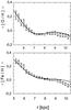 |
Fig. 1 Open squares are the averaged observed radial distributions of oxygen (upper panel) and iron (bottom panel) derived using Cepheids in the Milky Way (data taken from AMK). The error-like bars are the standard deviations of the corresponding mean values. The solid lines are the best-fit theoretical radial abundance distributions (see Sect. 3.1). |
The radial distribution of oxygen demonstrates a sufficiently sharp break in its behaviour near r ~ 7 kpc (for the solar Galactocentric distance, we adopt r0 ≡ 7.9 kpc). However, for iron, there is no sharp bend in the gradient at the same distance, although it is still clear that its distribution cannot be satisfactorily described by a singular linear function. In what follows, we restrict ourselves to radii r ≤ 10.5 kpc.
2.2. Equations for the chemical evolution of the ISM
The formalism employed to model the chemical evolution of the Galactic disk is based on the classical 1D (radial) approach of Tinsley (1980): ![Mathematical equation: \begin{eqnarray} \dot{\mu}_{\rm g} &=&f-\psi + \int\limits_{m_{\rm L}}^{m_{\rm U}}{(m-m_{\rm w})\psi(t-\tau_{\rm m})\phi (m)\,{\rm d}m}, \\[2mm] {\dot{\mu}_j}&=&\int\limits_{m_{\rm L}}^{m_{\rm U}}{(m-m_{\rm w})\,Z_j(t-\tau_m) \psi(t-\tau_m)\phi (m)\,{\rm d}m} \nonumber\\[2mm] &&+E_j^{\rm Ia}+E_j^{\rm cc} + fZ_{j,{\rm f}}-Z_j\psi +\frac{1}{r} \frac{\partial {}}{\partial r} \left(r\mu_{\rm g} D\frac {\partial Z_j}{\partial r}\right)\cdot \end{eqnarray}](/articles/aa/full_html/2013/09/aa20944-12/aa20944-12-eq18.png) Here, μg is the surface mass density of the interstellar gas (ISG), f = f0exp( − r/rd − t/tf) is the infall rate of intergalactic gas onto the Galactic disk with temporal and radial scales of tf = 2 Gyr (AMR) and rd = 3.5 kpc (Marcon-Uchida et al. 2010), respectively; f0 is computed using the normalizing condition that the total surface density of the Galactic disk (stellar + gaseous) at the Sun’s galactocentric distance r0 at the present epoch (t = TD = 10 Gyr, where TD is the age of the disk) is 50 M⊙ pc-2 (Haywood et al. 1997; Portinari & Chiosi 1999); ψ is the star formation rate (SFR), m the stellar mass (in solar mass units), τm the lifetime of a star of mass m (in Gyr), where log (τm) = 0.9 − 3.8log (m) + log 2(m) (Tutukov & Kruegel 1980; cf. Fig. 1 of Gibson 1997), and φ(m) the adopted Kroupa et al. (1993) initial mass function (IMF). The mass of stellar remnants mw (white dwarfs, neutron stars, and black holes) is as follows: for m ≤ 10, mw = 0.65m1/3; in the range 10 < m < 30, mw = 1.4 (neutron star); for 30 ≤ m < mU, the remnant is assumed to be a black hole of mw = 10; finally, for m ≥ mU = 70 the stars are assumed to collapse to black holes immediately after their birth and are removed from future chemical evolution (Tsujimoto et al. 1995). The lower stellar mass limit is taken to be mL = 0.1 M⊙, μj is the surface mass density of oxygen or iron (j = O or j = Fe, respectively), Zj = μj/μg is the mass fraction for the elements in the interstellar medium, Zj,f is the metallicity of the infalling gas, and t is time. The last term in Eq. (2) describes the radial diffusion of the elements; the expression for the diffusion coefficient D is given by Acharova et al. (2010).
Here, μg is the surface mass density of the interstellar gas (ISG), f = f0exp( − r/rd − t/tf) is the infall rate of intergalactic gas onto the Galactic disk with temporal and radial scales of tf = 2 Gyr (AMR) and rd = 3.5 kpc (Marcon-Uchida et al. 2010), respectively; f0 is computed using the normalizing condition that the total surface density of the Galactic disk (stellar + gaseous) at the Sun’s galactocentric distance r0 at the present epoch (t = TD = 10 Gyr, where TD is the age of the disk) is 50 M⊙ pc-2 (Haywood et al. 1997; Portinari & Chiosi 1999); ψ is the star formation rate (SFR), m the stellar mass (in solar mass units), τm the lifetime of a star of mass m (in Gyr), where log (τm) = 0.9 − 3.8log (m) + log 2(m) (Tutukov & Kruegel 1980; cf. Fig. 1 of Gibson 1997), and φ(m) the adopted Kroupa et al. (1993) initial mass function (IMF). The mass of stellar remnants mw (white dwarfs, neutron stars, and black holes) is as follows: for m ≤ 10, mw = 0.65m1/3; in the range 10 < m < 30, mw = 1.4 (neutron star); for 30 ≤ m < mU, the remnant is assumed to be a black hole of mw = 10; finally, for m ≥ mU = 70 the stars are assumed to collapse to black holes immediately after their birth and are removed from future chemical evolution (Tsujimoto et al. 1995). The lower stellar mass limit is taken to be mL = 0.1 M⊙, μj is the surface mass density of oxygen or iron (j = O or j = Fe, respectively), Zj = μj/μg is the mass fraction for the elements in the interstellar medium, Zj,f is the metallicity of the infalling gas, and t is time. The last term in Eq. (2) describes the radial diffusion of the elements; the expression for the diffusion coefficient D is given by Acharova et al. (2010).
We take the edge of the Galactic disk to be r = RG ≡ 25 kpc; for the initial conditions, we assume μg(t = 0) = 0 and Zj(t = 0) = Zj,f. We experimented with various initial fractions (ZO,f/ZO, ⊙ = 0.02, 0.05, and 0.1), with the adopted fraction for iron being ZFe,f = 0.02 ZFe, ⊙. Parameter space studies such as these allow us to assess the sensitivity of the results, especially the predicted [O/Fe] ratio, to the conditions at the epoch of Galactic disk formation (e.g. Renda et al. 2005; Fuhrmann & Bernkopf 2008).
The enrichment rates  of the Galaxy for the jth chemical element due to the explosion of the ith type of SNe – CC SNe (i = cc) or SNeIa (i = Ia) are given by the expression (Tinsley 1980)
  (3)where Ri is the rate of the ith type of SN explosions per unit of surface area, and
  is the mean mass of the jth element ejected per ith type of SN event. The above mean ejected masses
  are our target free parameters.
To close the equations, a Schmidt–like approximation for the star formation is often adopted (i.e.  , with k ~ 1.5: Kennicutt 1998). However, to explain the formation of the structure in the radial gradient of oxygen (and iron), we adopt a formalism for ψ which explicitly takes into account the effects of the spiral arms. We follow the prescription proposed by Wyse & Silk (1989; hereafter WS) and Portinari & Chiosi (1999; hereafter PC) which is based on the popular suggestion that Galactic spiral shocks stimulate star formation (e.g. Roberts 1969; Shu et al. 1972). In this prescription, the functional form follows
  , where Ω(r) is the angular rotation velocity of the Galactic matter and ΩP is the rotation velocity of the Galactic spiral waves responsible for the arms. WS and PC assume that: (i) Galactic spiral shocks stimulate formation of stars of all masses (both high and low), and (ii) the co-rotation resonance rc where Ω(rc) = ΩP, is situated at the edge of the Galactic disk (Lin et al. 1969). In what follows, we adopt the aforementioned equations of galactic chemical evolution, including the effects of spiral arms, under the assumption that spiral arms stimulate formation of sufficiently massive stars, but now considering the case for which the corotation resonance is situated close to the Sun2.
2.3. Formation of the Galactic gaseous disk
Until recently, little consensus existed as to the role of spiral arms in triggering star formation across the full spectrum of stellar masses. For our work, though, what is important is whether or not the sources of heavy elements are concentrated within the arms at the moment of ejection of the synthesized elements to the surrounding ISM. Observations do demonstrate that CC SNe are strongly associated with the spiral arms (Bartunov et al. 1994; Li et al. 2011). Progenitors of CC SNe are massive stars (m > 8 M⊙) with very short lifetimes (τ ≲ 20 Myr). As such, they have not had sufficient time to move significantly from their birth location within the arm. Conversely, as noted in Sect.1, the progenitors of SNeIa-T have lifetimes in excess of ~100 Myr (up to several Gyr or more; Matteucci & Greggio 1986). Even if these (lower mass) progenitors were born in the spiral arms, by the time of their explosion they now appear uniformly distributed in Galactic azimuth (Mishurov & Acharova 2011). Finally, SNeIa-P are strongly associated with the spiral arms (Bartunov et al. 1994; Li et al. 2011) and the ages of their progenitors may be estimated to be ≲100 Myr3. (Mannucci et al. 2005, 2006; Matteucci et al. 2006; Maoz et al. 2010; cf. Matteucci & Greggio 1986).
Since the mass of a single star with lifetime ~100 Myr is ~4 M⊙, we split the star formation rate (SFR) into the rates of high and low stellar mass formation (ψH and ψL), for m > 4 M⊙ and m < 4 M⊙, respectively. Using  , we re-cast the second term in the right hand-side of Eq. (1) as
  (4)Here, m = 100 M⊙ is the upper mass limit for stars at the time of their birth (Romano et al. 2005), whereas mU = 70 in Eqs. (1) and (2) is the upper mass of stars which take part in the Galactic matter circulation.
In the classical 1D approach to chemical evolution, it is impossible to consider the scattering of long-lived stars over the Galactic disk (cf. Mishurov & Acharova 2011). As such, we assume that low mass stars are not concentrated within spiral arms (a fairly conservative assumption given the reasonably long lifetimes of these stars). What this means is that for ψL we use the usual star formation formalism  (5)where ν is a normalizing coefficient (see below).
As was shown by Bartunov et al. (1994) and Anderson et al. (2012), CC SNe are tightly linked with HII regions and their azimuthal distributions are consistent with density and/or galactic shock waves (e.g. Roberts 1969; Boeshaar & Hodge 1977). Hence, the formalism for ψH may be written as  , where Π = αexp [ − (θ − θs)/δ ] represents the profile of the galactic shock with azimuth angle θ; α is the peak value of Π at the shock front, θs the location of the shock, and δ the typical width of an arm in units of Galactic azimuth (Fig. 2). This formalism is valid for θs < θ < θs + π; for other angles, the expression for Π is derived by means of a periodicity condition.
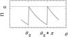 |
Fig. 2 Schematic dependence of Π on θ, where θs is the location of the shock front and α is the peak value of Π at the shock front. |
To pass from 2D (r,θ-representation) to 1D (r-representation), we average ψH over θ and derive
 The shock intensity is well-approximated by α ∝ r | (Ω − ΩP) | (Roberts et al. 1975) and δ can be estimated as δ ≈ (d/r)sin(p), where p is the pitch angle of a spiral arm and d is the typical width of an arm in the direction perpendicular to it. It is easy to show that δ < 1. This then yields the same approximation for ψH which was proposed by WS and PC
 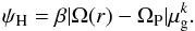 (6)Here, the coefficient β includes the constants of proportionality which enter the above model representations.
In the end, Eq. (1) can be reduced to the form ![Mathematical equation: \begin{eqnarray} \dot{\mu}_{\rm g}(r,t)&=&f(r,t)-\psi_{\rm L}(r,t)\int _{m_{\rm L}}^{4}m\phi {\rm d}m \nonumber\\ &&+\int\limits_{m_{\rm L}}^{m_{\rm U}}{(m-m_{\rm w})\psi_{\rm L}(r,t-\tau_m)\phi (m)\,{\rm d}m} \\ &&-\,\psi_{\rm H}(r,t)[\int\limits_{m_{\rm U}}^{100}\phi(m) {\rm d}m + \int\limits_{4}^{m_{\rm U}}m_{\rm w}\phi(m) {\rm d}m]\nonumber. \end{eqnarray}](/articles/aa/full_html/2013/09/aa20944-12/aa20944-12-eq99.png) (7)Here, for massive stars we use explicitly the instantaneous recycling approximation.
(7)Here, for massive stars we use explicitly the instantaneous recycling approximation.
In the computations which follow, we use the rotation curve based on that of Clemens (1985), adjusted for the adopted scale:
![Mathematical equation: $$ r\Omega(r) = 260 \exp \left\{-\left[\frac{r}{150}+\left(\frac{3.6}{r}\right)^2\right] \right\} + 360 \exp \left[-\left(\frac{r}{3.3}+\frac{0.1}{r}\right)\right]\cdot $$](/articles/aa/full_html/2013/09/aa20944-12/aa20944-12-eq100.png) The rotation curve with the adopted ΩP = 33 km s-1 kpc-1 is shown in Fig. 3. The corotation resonance is situated at rc ~ 7 kpc (AMR, AMK). In the expression for ψH, we introduce a cut-off factor at the outer Lindblad resonance rout which exponentially decreases beyond the resonance with a scale ~0.5 kpc, whereas following WS and PC we do not restrict the region of massive star formation by the inner Lindblad resonance4.
The rotation curve with the adopted ΩP = 33 km s-1 kpc-1 is shown in Fig. 3. The corotation resonance is situated at rc ~ 7 kpc (AMR, AMK). In the expression for ψH, we introduce a cut-off factor at the outer Lindblad resonance rout which exponentially decreases beyond the resonance with a scale ~0.5 kpc, whereas following WS and PC we do not restrict the region of massive star formation by the inner Lindblad resonance4.
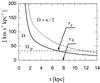 |
Fig. 3 Rotation curve (solid line) plotted alongside Ω + κ/2 (dotted line, where κ is the epicyclic frequency). The vertical dotted line shows the location of the outer Lindblad resonance (at rout ~ 11.5 kpc). |
Equations (5) to (7) have two free parameters, ν and β. They are fitted so as to ensure the solution satisfies the two normalizing conditions: (i) μg(r0,TD) = μg0 = 10 M⊙ pc-2 (Haywood et al. 1997); and (ii) the computed theoretical frequency for CC SNe events in our Galaxy at the present epoch  equates to the observed value:
  per century (Li et al. 2011).
The theoretical frequencies for the ith type of SNe event  are computed through the corresponding rates Ri as
  (8)where RG ≡ 25 kpc is the adopted radial extent of the Galaxy and the rate for CC SNe events is
  (9)where
  is the upper limit to the initial mass of CC SNe progenitors. Since its value is not known a priori, initially we adopt
  .
.
Finally, to solve the above equations and derive μg(r,t) we employ the following iterative procedure. At the first step, we suppose that β = 0 and solve the corresponding equations for a set of ν, seeking the minimum of the discrepancy Δμ = [ μg(r0,TD) − μg0 ] 2. Then, for the μg(r,TD) which corresponds to minΔμ, we compute the theoretical frequency , equate it to the observed frequency  , and derive β. After that we repeat the numerical solution of the above equations with the renewed β for a set of ν, determine the new ν corresponding to minΔμ, and calculate the corrected β. This procedure is repeated iteratively until convergence is reached. For the starting value of mcc = 70 M⊙, the free parameters inferred are
  pc-2 Gyr-1 and
  pc (their corrected values will be given in Sect. 3.1). In Fig. 4 we show the temporal evolution of the gaseous density for the final parameters after their corrections (see Sect. 3.1 for details)5.
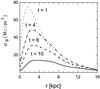 |
Fig. 4 Temporal evolution of the radial gas surface density distribution μg(r,t); see text for details. |
2.4. Rates of SNeIa events
Tardy SNeIa are not concentrated in spiral arms, and we describe their event rate usually as 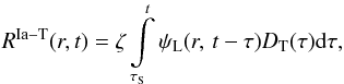 (10)where DT is the part of the delay time distribution (DTD) function for the tardy sub-population (Mannucci et al. 2006; Matteucci et al. 2006; Maoz et al. 2010) and τ is the time delay between the birth of a corresponding progenitor and its explosion (below we give the results for the smooth DTD function of Maoz et al. 2010; the results for the bimodal function of Mannucci et al. 2006 are close to those described below). The constant ζ is derived by means of computing
  and equating it to
  .
.
Since the prompt sub-population is concentrated in spiral arms, their event rate is functionally comparable to that of the CC SNe, 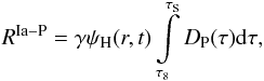 (11)where DP is the part of DTD function corresponding to SNeIa-P (see Maoz et al. 2010 and AMK) and γ is a normalizing constant which is determined by means of equating the theoretical and observed frequencies for SNeIa-P events.
According to Li et al. (2011) the observed frequency of SNeIa today  is ~0.54 per century. Using their ratio
 we find
  and
and  per century. The above authors note that their values may have systematic uncertainties up to a factor of ~2. As such, the errors in observations carry the most weight in the search for the optimal parameters.
2.5. Statistical method for deriving the radial distribution of oxygen and iron
Having inferred the dependence of μg(r,t) on the fixed parameters , we can solve numerically for the chemical evolution using Eq. (2). To derive the target parameters we minimize the discrepancy function ΔX over ![Mathematical equation: \begin{eqnarray} \Delta^2_X = \frac{1}{n-p}\sum_{k\,=\,1}^n\left\{ \left(\left\langle [X/{\rm H}]^{\rm obs} \right\rangle_k - [X/{\rm H}]^{\rm th}_k\right)w_k\right\}^2, \end{eqnarray}](/articles/aa/full_html/2013/09/aa20944-12/aa20944-12-eq140.png) (12)where the superscript “obs” corresponds to the observational data and “th” to the theoretical data, wk is a weight (we assume it to be inversely proportional to the length of the error-like bar in the kth bin, as in Fig. 1), n = 20 the number of bins, p the number of free parameters, and the summation is taken over all kth points within the adopted Galactocentric radius range.
(12)where the superscript “obs” corresponds to the observational data and “th” to the theoretical data, wk is a weight (we assume it to be inversely proportional to the length of the error-like bar in the kth bin, as in Fig. 1), n = 20 the number of bins, p the number of free parameters, and the summation is taken over all kth points within the adopted Galactocentric radius range.
The procedure can now be considered in more detail. Since oxygen is mainly produced by CC SNe and we can neglect the contributions from other sources (see AMR and AMK, and references therein), the calculations for this element are performed separately. To find the minimum of the discrepancy function, we solve numerically Eq. (2) for a set of  (and
(and  ), varying its value over a wide range at some step, and then compute the theoretical distribution at t = TD for each ejected mass of oxygen. next, by means of Eq. (12), we derive the dependence of ΔO as a function of and search for its minimum. In this way, we derive the first free parameter independently of the others (in this case, p = 1).
In contrast, iron is produced by three sources, CC SNe, SNeIa-P, and SNeIa-T. Tardy SNeIa do not concentrate within spiral arms; rather, they contribute to the radial distribution of iron with an approximately constant gradient. Unlike tardy SNeIa, CC SNe and prompt SNeIa are concentrated in spiral arms and are responsible for the inflection in the radial abundance gradients. It is obvious from Eqs. (9) and (11) that the rates Rcc and RIa − P have very close functional dependencies on r. Therefore, it is impossible to distinguish their contributions by means of statistical analyses if we do not introduce any a priori assumptions, which in statistics is referred to as the multi-collinearity problem. Therefore, we can only indicate the upper values of  and
and  .
.
To describe the algorithm for the search of the mean ejected masses of iron we write the corresponding enrichment rate of the Galactic disk by the element EFe in explicit form:  (13)Next, we suppose that
  ; substituting EFe into Eq. (2), we solve for a set of pairs
  , compute the radial distribution of iron at t = TD, and find the minimum of the discrepancy ΔFe that gives the best parameters of
  and
and  .
.
At the second step, we assume that  , again solve numerically Eq. (2) for a set of pairs
  , compute the radial distribution of iron, and seek the minimum of the discrepancy ΔFe that now gives the best parameters of
  and . Thus, we derive the best value for , , and (at this step in the treatment of iron, p = 2).
The above estimates for the mean masses of iron ejected by CC SNe or SNeIa-P are only upper limits since it is impossible to separate their simultaneous contributions, unless we possess additional information.
3. Results and discussion
3.1. Oxygen
As noted in Sect. 2.2, we performed several experiments with various initial values for ZO(t = 0), the results of which show this choice does not have an impact on our conclusions. The application of the aforementioned modelling of the observed oxygen distribution results in a predicted mean mass of  M⊙ ejected per CC SNe event6. This value differs significantly from the ones (1.8–3.7 M⊙) proposed by Woosley & Weaver (1995, hereafter WW95), Tsujimoto et al. (1995, hereafter T95), and Thielemann et al. (1996)7. We now discuss the reason for this divergence and the consequence of the predicted lower mean ejected mass of oxygen per CC SNe event.
To estimate  , one needs the mass-dependent oxygen yields from the relevant stellar evolution grid, and then to convolve that with an appropriate IMF and its associated upper limit for stars ending their lives as CC SNe (e.g. mU ~ 50–70 M⊙, as in T95). We also assumed in Eq. (9) that
  (see Sect. 2.3), but this was adopted solely as an initial guess. We will now define more accurately. For this, we use the procedure close to the one described by Gibson (1998) where the mean mass of oxygen ⟨ MO ⟩ ejected per CC SNe event (whose progenitor had the initial mass m) was represented as
 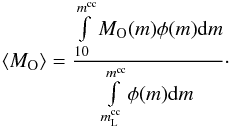 (14)We will not address the question of the lower limits in the above integrals. As argued by WW95 (see also T95), CC SNe of masses approximately in the interval 8–10 M⊙ contribute very little to the production of elements like oxygen. That is why the lower limit in the integral in the numerator is set to 10 M⊙. The authors (T95) use the same value (10 M⊙) for the lower limit in the integral entering the denominator in Eq. (14). We believe however that
  must be equal to the lower limit in the integral representing the rate of CC SNe events (see Eq. (9)), since the stars in the mass range 8–10 M⊙ contribute to the observed frequency of the corresponding CC SNe events (Li et al. 2011; Smartt et al. 2009). In other words, these stars influence the mean ejected mass of oxygen through the rate of CC SNe events. Hence, we should impose
  .
.
Using for MO(m) the yields published in the literature, we compute the dependence of ⟨ MO ⟩ as a function of mcc and, by equating  , we find the new upper initial mass, , of a star which can explode as a CC SNe. For
  and the yields of T95, the corrected initial mass comes to
  (see Fig. 5).
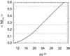 |
Fig. 5 Dependence of ⟨ MO ⟩ on mcc for the yields of T95. |
Furthermore, since the new differs from the initial value (70 M⊙), we have to launch the next iterative step. For this, we substitute the new value  into Eq. (9) and repeat the procedure from the beginning to solve anew the equations for evolution of μg, re-determine the constants ν, β, and , and derive the improved value for
  . Our calculations show that the corrected values of the constants are
  pc Gyr-1,
  pc (the dependence of μg(r,t) for these final parameters is shown in Fig. 4), and
  . The corresponding mean ejected mass of oxygen happens to be slightly less than the previous value
  (see Fig. 5). To estimate the scatter in due to the uncertainty in the observed frequency of CC SNe events, we adopt a value for
  two times greater (or lower) than the best value of Li et al. (2011). Correspondingly, will be a factor of two lower (or greater) than the above derived value. By means of Fig. 5, we find
  . If we use the yields of Hirschi et al. (2005), will be systematically lower by ~2 M⊙8. The theoretical radial distribution of oxygen in the Galactic disk, superimposed on the observed distribution, is shown in Fig. 1.
The above upper initial mass for CC SNe progenitors is close to that favoured by Maeder (1992) and Heger et al. (2003) who proposed an upper initial mass limit for exploding SNe to be ~20–25 M⊙. Moreover, on the basis of observations, Smartt et al. (2009) insist that the progenitors of exploded CC SNe have masses below ~17 M⊙. Eldridge et al. (2013) also do not find evidence for the existence of very massive stars (~100 M⊙) which might be considered as progenitors for observed SNe Ib/c. Finally, Kochanek et al. (2008) suggest that stars more massive than the above transform directly to black holes at the end of nuclear burning without exploding (or undergoing a backward explosion).
For our theory it is crucial that, independent of the final stages of stellar evolution, stars with very large initial masses do not necessarily explode as CC SNe. In our picture, if they did, they would supply too much oxygen to the Galactic disk. In our approach, we are not faced with the problem of an excessive frequency of CC SNe events, noted by Brown & Woosley (2012), since the observed frequencies are built into the theory at the time of disk formation.
3.2. Iron
After improvements associated with a more precise definition of , we derive the final values γ = 0.0061 and ζ = 0.0007. The mean mass of iron ejected per SNeIa–T event is  and it is approximately the same, independent of the type of short-lived SNe excluded (core-collapse or prompt SNeIa, see Sect. 2.5). This is expected, since tardy SNeIa are responsible for the quasi-linear radial distribution of iron along the Galactic disk.
In addition, if , then the mean mass of iron ejected per CC SNe event is  whereas for the case , the corresponding mass ejected per prompt SNeIa event is
  (for the corresponding theoretical radial distribution of iron, see Fig. 1)9.
As mentioned in Sect. 1, SNeIa are usually associated with long-lived objects and the yields of iron, estimated on the basis of a theory of pre-SNeIa evolution (e.g. Nomoto et al. 1997; Iwamoto et al. 1999; Umeda & Nomoto 2002; Limongi & Chieffi 2003; Kobayashi et al. 2006; Tominaga et al. 2006; Woosley et al. 2007), are derived without separation of SNeIa into prompt and tardy sub-populations. Our estimates of the mean mass, ejected by prompt and tardy SNeIa per respective event, are the first indication that these sub-populations do produce different amounts of iron. If the events arise in similar conditions (white dwarfs, the progenitors of SNeIa, have masses in a very narrow range), how can this be understood? Perhaps the discrepancy may be explained by the weak dependence between the peak luminosity and explosion kinetic energy for most SNeIa (Blondin et al. 2012), or perhaps SNeIa-P undergo asymmetric explosions (Maeda et al. 2010)?
The low mean mass of iron ejected per core-collapse SNe event (~0.04 ± 0.01 M⊙) is close to the observed mass given by Smartt et al. (2009), 0.01–0.03 M⊙, for carefully measured CC SNe. Hence, an even more challenging assumption might be to speculate that perhaps the nature of prompt SNeIa is not associated with white dwarfs, but rather with CC SNe. Indeed, as was noted in Sect. 1, observations show that young SNeIa-P are brighter than old tardy SNeIa, but according to our results prompt SNeIa produce (per event) about 2.5 times less iron than tardy SNeIa. How can this inverse correlation be explained if the main source of SNeIa luminosity is thought to be the decay of nickel to iron which is synthesized in a process with similar characteristics to that of the Chandrasekhar limit for white dwarfs? The low values of iron produced by CC SNe and SNeIa-P make it tempting to give credence to our suggestion. Besides, it is well known that, like core-collapse SNe, prompt SNeIa are concentrated in sites of star formation within spiral arms (Bartunov et al. 1994; Mannucci et al. 2005; Panagia et al. 2007; Li et al. 2011). Hence, we may assume that their progenitors were sufficiently massive stars. Moreover, in a recent paper Foley et al. (2012) have revealed, for the first time, strong outflows from SNeIa progenitors in late-type galaxies, but in early-type galaxies these outflows are extremely rare. If we recall that in early galaxies we observe old (i.e. tardy) SNeIa but in late-type galaxies one sees young (prompt) SNeIa, we might conclude that the phenomenon of Foley et al. provides a “link” between SNeIa-P and CC SNe. Further, it is worth noting the work of van Rossum (2012) who, on the basis of recent data, demonstrates that some features in SNeIa spectra may be interpreted incorrectly (e.g. emission may be interpreted as absorption). In some cases, this may mislead the classification of SNe type.
Our experiments enable us to estimate the total number of SNe Ni exploded in the Galaxy throughout its life: Ncc ~ 12.2 × 10⁸; NIa − P ~ 2.3 × 10⁸; and NIa − T ~ 0.2 × 10⁸. From these, we can estimate that short-lived SNe (CC or Ia-P) supply to the Galaxy ~85% of its iron. Correspondingly, SNeIa-T supply ~15% of the iron.
The low value inferred for the amount of iron supplied to the Galaxy by the long-lived sub-population of SNeIa differs from the one typically discussed in the literature. Indeed, prior to the most recent decade, SNeIa were essentially considered to be exclusively long-lived objects, and under this picture, they were thought to supply ~60% of the iron to the Galaxy (Gibson 1998; Matteucci 2004). This stance has changed since the discovery of the two sub-populations of SNeIa (short- and long-lived)10. As was shown by AMK, the relative portion of iron supplied to the Galaxy by tardy SNeIa reduced to ~35%, since the rapid SNeIa (and/or CC SNe) also contribute to iron synthesis. According to our work here, the contribution of long-lived SNeIa to the disk’s iron enrichment appears a factor of ~2 lower than even this reduced fraction. This is mainly a consequence of our new model for the SFR function ψ which we explicitly split into low and high massive star formation rates, the mathematical representations for these two parts being very different. This modification drives the relatively low amount of iron contributed to the Galactic disk and ejected per tardy SNeIa event to ~0.4–0.8 M⊙.
Although our yields are derived in the context of a galactic chemical evolution model for the Galactic disk, it is tempting to extend their application to the stellar halo. Indeed, such stars are to be enriched primarily by earlier generations of short-lived SNe. Can we explain the enhanced ratios of [α/Fe] in halo stars via the use of our empirically inferred yields? If we assume that the enrichment seen in the oxygen and iron abundances of halo stars was due to CC SNe only, one can estimate the expected ratio as being ![Mathematical equation: \hbox{${\rm [O/Fe]}=\log\,(P^{\rm cc}_{\rm O}/m_{\rm O})- \log\,(P^{\rm cc}_{\rm Fe}/m_{\rm Fe})- \log {\rm (O/Fe)}_{\odot}$}](/articles/aa/full_html/2013/09/aa20944-12/aa20944-12-eq197.png) , where mO and mFe are the atomic masses of oxygen and iron, respectively; for the solar ratio in our work we adopt log (O/Fe)⊙ = 1.19 (in all our work we employ the solar scale of Asplund et al. 2009, since this scale was also used in the determination of the elemental patterns from the aforementioned Cepheid samples). For the above yields, we derive [O/Fe] = +0.18 (for the lower value of
, where mO and mFe are the atomic masses of oxygen and iron, respectively; for the solar ratio in our work we adopt log (O/Fe)⊙ = 1.19 (in all our work we employ the solar scale of Asplund et al. 2009, since this scale was also used in the determination of the elemental patterns from the aforementioned Cepheid samples). For the above yields, we derive [O/Fe] = +0.18 (for the lower value of  , the ratio comes to [O/Fe] = +0.31). While our framework was not created with the stellar halo in mind, it is at least re-assuring to note that under the assumption of rapid enrichment, our inferred estimates of the resulting [α/Fe] are not dissimilar to the ~+0.2−0.3 dex α-enhancements seen in typical metal-poor environments. Furthermore, we should re-iterate that our quoted mean mass of iron ejected per CC SNe event is technically only an upper limit. We hope that a more careful analysis that explicitly takes into account the evolutionary history of halo, like in Renda et al. (2005), will enable us to better apply our preliminary work outside of the regime for which it has been optimised here. Stronger observational constraints on various sub-types of SNe, particularly in distant galaxies, are also critical, as for example the data of Li et al. (2011) provides insights really only into the SNe rates today, rather than as a function of time.
There may be another way to explain the enhanced α/Fe ratio in halo stars; specifically, because the very low metallicity (Z ~ 0.001 Z⊙) at the epoch of halo formation, the initial masses of CC SNe may be higher (~40 M⊙) than the masses of CC SNe exploding in the Galactic thin disk. According to Maeder (1992) these CC SNe progenitors produce several times more oxygen than their counterparts at solar metallicity.
4. Conclusions
Our goal was to derive the mean masses of oxygen and iron ejected per each sub-type of SNe, and, as a consequence, the constraints on some properties of their progenitors. For this, we refined the statistical analysis of the observed (non-linear) radial distributions of elements in the Galactic disk previously developed by AMR and AMK. Breaking with the traditional approach of adopting tabular nucleosynthetic yields in the chemical evolution modelling, we instead derive them a posteriori, within our framework (Sect. 2).
The results are as follows:
-
The mean mass of oxygen ejected perCC SNe eventis ~0.27 M⊙, while the upper value for the mass of iron ejected by this type of SNe is ~0.04 M⊙.
-
The mean mass of iron ejected by tardy SNeIa (progenitors which are long-lived with ages from ~100 Myr up to several Gyrs, and which are not concentrated in spiral arms) is ~0.58 M⊙ per event. Conversely, prompt SNeIa (progenitors that are short-lived with ages ≲100 Myr and which are concentrated within spiral arms) on average supply ≤0.24 M⊙ per event to the Galactic disk.
-
Short-lived SNe (core-collapse and prompt Ia) supply ~85% of the iron to the Galactic disk.
The low amount of oxygen ejected per CC SNe leads us to the conclusion that the maximum initial mass of exploding CC SNe progenitors is ≤23 . This result supports the inferences of Heger et al. (2003), Kochanek et al. (2008), and Smartt et al. (2009); i.e. that stars of initial masses greater than about 17–25 M⊙ do not explode and, as such, they do not return the bulk of their newly synthesized material to the ISM. Perhaps, they collapse to black holes shortly after their birth without explosion or undergo a backward explosion. As a consequence, they do not take part in Galactic nucleosynthesis (except perhaps through their pre-SN stellar wind mass-loss).
The mean mass of iron ejected by the typical CC SNe (≤0.04 M⊙) is close to the empirical values favoured by Smartt et al. (2009). The mean masses of iron ejected by prompt and tardy SNeIa appear to be different. It is surprising that the older and less energetic tardy SNeIa produce about 2.5 times more iron (per event) than prompt SNeIa, which are younger and more energetic objects (Gonzalez-Gaitan et al. 2011). This suggests that perhaps, in their nature, SNeIa-P are closer to core-collapse SNe than to those whose explosions are associated with the thermonuclear burning of a Chandrasekhar mass white dwarf.
To cross an interarm distance, it takes the time interval ~π |Ω − ΩP| -1 ~ 100 Myr. Therefore, we can adopt this as the boundary value separating the prompt short-lived sub-population of SNeIa that concentrates in spiral arms from tardy long-lived SNeIa that do not concentrate in arms.
Khoperskov et al. (2012) showed that the inner Lindblad resonance has little influence on spiral density wave generation.
In our previous papers (e.g. AMR and AMK) we followed literatim, the idea of Oort (1974) and introduced the factor | Ω − ΩP | into the enrichment rates  and
and  as an additional multiplier retaining the same Schmidt-like representation for SFR (
 ) for stars of all masses. But in the present paper, we explicitly split the star formation rate into low and high mass components and approximate them by different functional representations (cf. Eqs. (5) and (6)). As a consequence, we derive a radial density distribution for the gas which differs significantly from that obtained in our earlier work. In particular, we now predict a surface density distribution with a hole in the center which resembles closely the observed distribution shown by Dame (1993). These quantitative and qualitative changes have entailed the changes in the sought-for parameters.
The associated random error is much lower than the error due to the uncertainty in the observed frequencies of SNe events (Li et al. 2011). Hence, we neglect the random error in .
The low inferred value for is closer to the yields of Arnett (1991) and Langer & Henkel (1995); see Table 1 of Gibson, et al. (1997).
We note that the changes in the upper initial mass for the exploding CC SNe follow from the non-linear dependence of the mean ejected mass of oxygen on .
According to our definition (Sect. 2.3), SNeIa of ages more than ~400 Myr (Matteucci & Greggio 1986) are considered to be SNeIa-T.
Acknowledgments
The authors wish to thank A. Zasov, S. Blinnikov, D. Tsvetkov, and the anonymous referee for their valuable guidance. This work was supported by the Ministry of Education and Science of the Russian Federation (14.A18.21.0787 and 14.A18.21.1304) and the grant of the Southern Federal university. B.K.G. acknowledges the support of the UK Science and Technology Facilities Council (ST/J001341/1). I.A.A. thanks the Russian Funds for Basic Research scheme (12-02-90701-mob-st).
References
- Acharova, I., Lépine, J. R. D., & Mishurov, Yu. 2005a, MNRAS, 359, 819 [NASA ADS] [CrossRef] [Google Scholar]
- Acharova, I., Lépine, J. R. D., & Mishurov, Yu. 2005b, Astron. Report, 49, 354 [NASA ADS] [CrossRef] [Google Scholar]
- Acharova, I., Lépine, J. R. D., Mishurov, Yu., et al. 2010, MNRAS, 402, 1149 [NASA ADS] [CrossRef] [Google Scholar]
- Acharova, I., Mishurov, Yu., & Rasulova, M. 2011, MNRAS, 415, L11 (AMR) [NASA ADS] [CrossRef] [Google Scholar]
- Acharova, I., Mishurov, Yu., & Kovtyukh, V. 2012, MNRAS, 420, 1590 (AMK) [NASA ADS] [CrossRef] [Google Scholar]
- Anderson, J. P., Habergham, S. M., James, P. A., & Hamuy, M. 2012, MNRAS, 424, 1372 [NASA ADS] [CrossRef] [Google Scholar]
- Andrievsky, S., Kovtyukh, V., Luck, R., et al. 2002a, A&A, 381, 32 [NASA ADS] [CrossRef] [EDP Sciences] [Google Scholar]
- Andrievsky, S., Bersier, D., Kovtyukh, V., et al. 2002b, A&A, 384, 140 [NASA ADS] [CrossRef] [EDP Sciences] [Google Scholar]
- Andrievsky, S., Kovtyukh, V., Luck, R., et al. 2002c, A&A, 392, 491 [NASA ADS] [CrossRef] [EDP Sciences] [Google Scholar]
- Arnett, D. 1991, in Frontiers of Stellar Evolution, ed. D. L. Lambert, ASP Conf. Ser., 389 [Google Scholar]
- Asplund, M., Grevesse, N., Sauval, A. J., & Scott, P. 2009, ARA&A, 47, 481 [NASA ADS] [CrossRef] [Google Scholar]
- Boeshaar, G. O., & Hodge, P. W. 1977, ApJ, 213, 361 [NASA ADS] [CrossRef] [Google Scholar]
- Bartunov, O. S., Tsvetkov, D. Yu., & Filimonova, I. V. 1994, PASP, 106, 1276 [NASA ADS] [CrossRef] [Google Scholar]
- Blondin, S., Matheson, T., Kirshner, R., et al. 2012, AJ, 143, 126 [NASA ADS] [CrossRef] [Google Scholar]
- Bresolin, F., Ryan-Weber, E., Kennicutt, R. C., & Goddard, Q. 2009, ApJ, 695, 580 [NASA ADS] [CrossRef] [Google Scholar]
- Brown, J. M., & Woosley, S. E. 2013, ApJ, 769, 99 [NASA ADS] [CrossRef] [Google Scholar]
- Crowther, P., Schnurr, O., Hirschi, R., et al. 2010, MNRAS, 408, 731 [NASA ADS] [CrossRef] [Google Scholar]
- Crèzè, M., & Mennessier, M. O. 1973, A&A, 27, 281 [NASA ADS] [Google Scholar]
- Dame, T. M. 1993, in Back to the Galaxy, eds. S. Holt, & F. Verter, 267 [Google Scholar]
- Eldridge, J. J., Fraser, M., Smartt, S. M., & Crocett, R. M. 2013, MNRAS, accepted [arXiv:1301.1975] [Google Scholar]
- Foley, R., Simon, J., Burns, C., et al. 2012, ApJ, 752, 101 [NASA ADS] [CrossRef] [Google Scholar]
- Fuhrmann, K., & Bernkopf, J. 2008, MNRAS, 384, 1563 [NASA ADS] [CrossRef] [Google Scholar]
- Gibson, B. K. 1997, MNRAS, 290, 471 [NASA ADS] [Google Scholar]
- Gibson, B. K. 1998, ApJ, 501, 675 [NASA ADS] [CrossRef] [Google Scholar]
- Gibson, B. K., Loewenstein, M., & Mushotzky, R. F. 1997, MNRAS, 290, 623 [NASA ADS] [Google Scholar]
- Gibson, B. K., Stetson, P. B., Freedman, W. L., et al. 2000, ApJ, 529, 723 [NASA ADS] [CrossRef] [Google Scholar]
- Gibson, B. K., Pilkington, K., Brook, C. B., Stinson, G. S., & Bailin, J. 2013, A&A, 554, A47 [NASA ADS] [CrossRef] [EDP Sciences] [Google Scholar]
- Gonzalez-Gaitan, S., Conley, A., Bianco, F., et al. 2011, ApJ, 727, 107 [NASA ADS] [CrossRef] [Google Scholar]
- Haywood, M., Robin, A. C., & Crèzè, M. 1997, A&A, 320, 440 [NASA ADS] [Google Scholar]
- Heger, A., Fryer, C. L., Woosley, S. E., Langer, N., & Hartmann, D. H. 2003, ApJ, 591, 288 [NASA ADS] [CrossRef] [Google Scholar]
- Hirschi, R., Meynet, G., & Maeder, A. 2005, A&A, 433, 1013 [NASA ADS] [CrossRef] [EDP Sciences] [Google Scholar]
- Howell, D. A., Sullivan, M., Brown, E. F., et al. 2009, ApJ, 691, 661 [NASA ADS] [CrossRef] [Google Scholar]
- Iwamoto, K., Brachwitz, F., Nomoto, K., et al. 1999, ApJS, 125, 439 [NASA ADS] [CrossRef] [MathSciNet] [Google Scholar]
- Kennicutt, R. C. 1998, ApJ, 498, 541 [NASA ADS] [CrossRef] [Google Scholar]
- Khoperskov, S. A., Khoperskov, A. V., Khrykin, I. S., et al. 2012, MNRAS, 427, 1983 [NASA ADS] [CrossRef] [Google Scholar]
- Kobayashi, C., Umeda, H., Nomoto, K., Tominaga, N., & Ohkubo, T. 2006, ApJ, 653, 1145 [NASA ADS] [CrossRef] [Google Scholar]
- Kochanek, C., Beacom, J., Kistler, M., et al. 2008, ApJ, 684, 1336 [NASA ADS] [CrossRef] [Google Scholar]
- Kroupa, P., Tout, C. A., & Gilmore, G. 1993, MNRAS, 262, 545 [NASA ADS] [CrossRef] [Google Scholar]
- Langer, N., & Henkel, C. 1995, Sp. Sci. Rev., 74, 343 [Google Scholar]
- Lépine, J. R. D., Mishurov, Yu. N., & Dedikov, S. Yu. 2001, ApJ, 546, 234 [NASA ADS] [CrossRef] [Google Scholar]
- Lewis, K. M., Lugaro, M., Gibson, B. K., & Pilkington, K. 2013, ApJ, 768, L19 [NASA ADS] [CrossRef] [Google Scholar]
- Limongi, M., & Chieffi, A. 2003, ApJ, 592, 404 [NASA ADS] [CrossRef] [Google Scholar]
- Lin, C. C., Yuan, C., & Shu, F. H. 1969, ApJ, 155, 721 [NASA ADS] [CrossRef] [Google Scholar]
- Lineweaver, C. H., Fenner, Y., & Gibson, B. K. 2004, Science, 303, 59 [NASA ADS] [CrossRef] [Google Scholar]
- Li, W., Chornock, R., Leaman, J., et al. 2011, MNRAS, 412, L1473 [NASA ADS] [CrossRef] [Google Scholar]
- Maeda, K., Benetti, S., Stritzinger, M., et al. 2010, Nature, 466, 82 [NASA ADS] [CrossRef] [PubMed] [Google Scholar]
- Mannucci, F., DellaValle, M., Panagia, N., et al. 2005, A&A, 433, 807 [NASA ADS] [CrossRef] [EDP Sciences] [Google Scholar]
- Mannucci, F., Della Valle, M., & Panagia, N. 2006, MNRAS, 370, 773 [NASA ADS] [CrossRef] [Google Scholar]
- Marino, R. A., Gil de Paz, A., Castillo-Morales, A., et al. 2012, ApJ, 754, A61 [NASA ADS] [CrossRef] [Google Scholar]
- Maoz, D., Keren, S., & Gal-Yam, G. 2010, ApJ, 722, 1879 [Google Scholar]
- Marcon-Uchida, M. M., Matteucci, F., & Costa, R. D. D. 2010, A&A, 520, A35 [NASA ADS] [CrossRef] [EDP Sciences] [Google Scholar]
- Marochnik, L. S., Mishurov, Yu. N., & Suchkov, A. A. 1972, ApSS, 19, 285 [Google Scholar]
- Matteucci, F. 2004, in Baryons in Dark Matter Halos, Proceedings of Science, eds. R. Dettmar, U., Klein, & P. Salucci, SISSA, Italy, 721 [Google Scholar]
- Matteucci, F., & Greggio, L. 1986, A&A, 154, 279 [NASA ADS] [Google Scholar]
- Matteucci, F., Panagia, N., Pipino, A., et al. 2006, MNRAS, 372, 265 [NASA ADS] [CrossRef] [Google Scholar]
- de Mink, S., Cantiello, M., Langer, N., et al. 2009, A&A, 497, 243 [NASA ADS] [CrossRef] [EDP Sciences] [Google Scholar]
- Mishurov, Yu., & Acharova, I. 2011, MNRAS, 412, 1771 [NASA ADS] [CrossRef] [Google Scholar]
- Mishurov, Yu. N., & Zenina, I. A. 1999, A&A, 341, 81 [NASA ADS] [Google Scholar]
- Mishurov, Yu. N., Pavlovskaya, E. D., & Suchkov, A. A. 1979, Sov. Astron., 23, 147 [Google Scholar]
- Mishurov, Yu. N., Zenina, I. A., Dambis, A. K., Melnik, A. M., & Rastorguev, A. S. 1997, A&A, 323, 775 [NASA ADS] [Google Scholar]
- Mishurov, Yu. N., Lépine, J. R. D., & Acharova, I. A. 2002, ApJ, 571, L113 [NASA ADS] [CrossRef] [Google Scholar]
- Moriya, T., Tominaga, N., Blinnikov, S., Baklanov, P., & Sorokina, E. 2011, MNRAS, 415, 199 [NASA ADS] [CrossRef] [Google Scholar]
- Nomoto, K., Iwamoto, K., Nakasato, N., et al. 1997, Nucl. Phys. A, 621, 467 [NASA ADS] [CrossRef] [Google Scholar]
- Oort, J. 1974, in The Formation and Dynamics of Galaxies, ed. J.R. Shakeshaft, Proc. IAU Symp., 58 (Dordrecht: Reidel), 375 [Google Scholar]
- Perlmutter, S., Aldering, G., Goldhaber, G., et al. 1999, ApJ, 517, 565 [NASA ADS] [CrossRef] [Google Scholar]
- Pilkington, K., Few, C. G., Gibson, B. K., et al. 2012, A&A, 540, A56 [NASA ADS] [CrossRef] [EDP Sciences] [Google Scholar]
- Portinari, L., & Chiosi, C. 1999, A&A, 350, 827 (PC) [NASA ADS] [Google Scholar]
- Renda, A., Kawata, D., Fenner, Y., & Gibson, B. 2005, MNRAS, 356, 1071 [NASA ADS] [CrossRef] [Google Scholar]
- Riess, A. G., Filippenko, A. V., Challis, P., et al. 1998, AJ, 116, 1009 [NASA ADS] [CrossRef] [Google Scholar]
- Roberts, W. W. 1969, ApJ, 158, 123 [NASA ADS] [CrossRef] [Google Scholar]
- Roberts, W. W., Roberts, M. S., & Shu, F. H. 1975, ApJ, 196, 381 [NASA ADS] [CrossRef] [Google Scholar]
- Romano, D., Chiappini, C., Matteucci, F., & Tosi, M. 2005, A&A, 430, 491 [NASA ADS] [CrossRef] [EDP Sciences] [Google Scholar]
- Shu, F. H., Milione, V., Gebel, W., et al. 1972, ApJ, 173, 557 [NASA ADS] [CrossRef] [Google Scholar]
- Smartt, S., Eldridge, J., Crockett, R., & Maund, J. 2009, MNRAS, 395, 1409 [NASA ADS] [CrossRef] [Google Scholar]
- Schnurr, O., Casoli, J., Chene, A.-N., Moffat, A. F. J., & St-Louis, N. 2008, MNRAS, 389, L38 [Google Scholar]
- Sullivan, M., Le Borgne, D., Pritchet, C. J., et al. 2006, ApJ, 648, 868 [NASA ADS] [CrossRef] [Google Scholar]
- Tinsley, B. M. 1980, Fund. Cosmic Phys., 5, 287 [Google Scholar]
- Thielemann, F.-K., Nomoto, K., & Hashimoto, M. 1996, ApJ, 460, 408 [NASA ADS] [CrossRef] [Google Scholar]
- Truran, J., Glasner, A., & Kim, Y. 2012, J. Phys. Conf. Ser., 337, 012040 [NASA ADS] [CrossRef] [Google Scholar]
- Tsujimoto, T., Nomoto, K., Yoshii, Y., et al. 1995, MNRAS, 277, 945 (T95) [NASA ADS] [CrossRef] [Google Scholar]
- Tutukov, A., & Krügel, E. 1980, Sov. Astron., 24, 539 [NASA ADS] [Google Scholar]
- Umeda, H., & Nomoto, K. 2002, ApJ, 565, 385 [NASA ADS] [CrossRef] [Google Scholar]
- van Rossum, D. R. 2012, ApJL, submitted [arXiv:1208.3781] [Google Scholar]
- Woosley, S., & Weaver, T. 1995, ApJS, 101, 181 (WW95) [NASA ADS] [CrossRef] [Google Scholar]
- Woosley, S., Kasen, D., Blinnikov, S., & Sorokina, E. 2007, ApJ, 662, 487 [NASA ADS] [CrossRef] [Google Scholar]
- Wyse, R., & Silk, J. 1989, ApJ, 339, 700 (WS) [NASA ADS] [CrossRef] [Google Scholar]
All Figures
|
Fig. 1 Open squares are the averaged observed radial distributions of oxygen (upper panel) and iron (bottom panel) derived using Cepheids in the Milky Way (data taken from AMK). The error-like bars are the standard deviations of the corresponding mean values. The solid lines are the best-fit theoretical radial abundance distributions (see Sect. 3.1). |
| In the text | |
|
Fig. 2 Schematic dependence of Π on θ, where θs is the location of the shock front and α is the peak value of Π at the shock front. |
| In the text | |
|
Fig. 3 Rotation curve (solid line) plotted alongside Ω + κ/2 (dotted line, where κ is the epicyclic frequency). The vertical dotted line shows the location of the outer Lindblad resonance (at rout ~ 11.5 kpc). |
| In the text | |
|
Fig. 4 Temporal evolution of the radial gas surface density distribution μg(r,t); see text for details. |
| In the text | |
|
Fig. 5 Dependence of ⟨ MO ⟩ on mcc for the yields of T95. |
| In the text | |
Current usage metrics show cumulative count of Article Views (full-text article views including HTML views, PDF and ePub downloads, according to the available data) and Abstracts Views on Vision4Press platform.
Data correspond to usage on the plateform after 2015. The current usage metrics is available 48-96 hours after online publication and is updated daily on week days.
Initial download of the metrics may take a while.