| Issue |
A&A
Volume 556, August 2013
|
|
|---|---|---|
| Article Number | A134 | |
| Number of page(s) | 16 | |
| Section | Planets and planetary systems | |
| DOI | https://doi.org/10.1051/0004-6361/201321777 | |
| Published online | 08 August 2013 | |
Migration and gas accretion scenarios for the Kepler 16, 34, and 35 circumbinary planets
1 Université de Bordeaux, Observatoire Aquitain des Sciences de l’Univers, BP 89, 33271 Floirac Cedex, France
e-mail: This email address is being protected from spambots. You need JavaScript enabled to view it.
2 Laboratoire d’Astrophysique de Bordeaux, BP 89, 33271 Floirac Cedex, France
3 Astronomy Unit, Queen Mary University of London, Mile End Road, London, E1 4NS, UK
Received: 26 April 2013
Accepted: 2 July 2013
Abstract
Context. Several circumbinary planets have been detected by the Kepler mission. Recent work has emphasized the difficulty of forming these planets at their observed locations due to perturbations by the binary. It has been suggested that these planets formed further out in their discs in more quiescent environments and migrated in to locations where they are observed.
Aims. We examine the orbital evolution of planets embedded in circumbinary disc models for the three systems Kepler-16, Kepler-34 and Kepler-35. The aims are: to explore the plausibility of a formation scenario in which cores form at large distances from the binaries and undergo inward migration and gas accretion as the gas disc disperses; to determine which sets of disc parameters lead to planets whose final orbits provide reasonable fits to the observed systems.
Methods. Using a grid-based hydrodynamics code we performed simulations of a close binary system interacting with circumbinary discs with differing aspect ratios, h, and viscous stress parameters α. Once the binary+disc system reaches quasi-equilibrium we embed a planet in the disc and examine its evolution under the action of binary and disc forces. We consider fully-formed planets with masses equal to those inferred from Kepler data, and low-mass cores that migrate and accrete gas while the gas disc is being dispersed.
Results. A typical outcome for all systems is stalling of inward migration as the planet enters the tidally-truncated inner cavity formed by the binary system. The circumbinary disc becomes eccentric through interaction with the binary, and the disc eccentricity forces the planet into a non-circular orbit. For each of the Kepler-16b, Kepler-34b and Kepler-35b systems we obtain planets whose parameters agree reasonably well with the observational data, but none of our simulations are able to produce highly accurate fits for all orbital parameters.
Conclusions. The final orbital configuration of a circumbinary planet is determined by a delicate interplay between the detailed stucture of the circumbinary disc and the orbital parameters of the planet as it migrates into the inner disc cavity. Simplified simulations such as those presented here provide support for a formation scenario in which a core forms, migrates inward and accretes gas, but accurate fitting of the observed Kepler systems is likely to require disc models that are significantly more sophisticated in terms of their input physics.
Key words: accretion, accretion disks / planets and satellites: formation / methods: numerical / hydrodynamics
© ESO, 2013
1. Introduction
Among the thousands of planet candidates discovered by Kepler, at the time of writing 6 of them are circumbinary planets which orbit around both components of a close binary system on a so-called P-type orbit. Kepler-16b was the first circumbinary planet discovered with Kepler (Doyle et al. 2011). It is a Saturn-mass planet with near-circular orbit and semi-major axis ap ~ 0.7 AU (measured from the centre of mass of the binary). The binary harbouring Kepler-16b has semi-major axis ab ~ 0.22 AU, eccentricity eb ~ 0.16 and mass ratio qb = MB / MA ~ 0.29, where MA and MB are the masses of the primary and secondary stars respectively. Interestingly, Kepler-16b is found to orbit just outside the long-term stability limit located at ~0.64 AU from the binary (Holman & Wiegert 1999). Two additional transiting circumbinary planets have been reported by Welsh et al. (2012) around Kepler-34 and Kepler-35: binary systems with stellar binary periods of 28 and 21 days, respectively. Kepler-34b has orbital period 289 days and mass ratio q = mp / M⋆ ~ 1.1 × 10⁻⁴, where M⋆ = MA + MB and mp is the planet mass. Kepler-35b has orbital period 131 days and mass ratio q ~ 7.5 × 10⁻⁴. The binary and planet parameters for these three systems are summarised in Table 1. More recent detections include the Neptune-sized circumbinary planet Kepler-38b (Orosz et al. 2012a), a system of 2 planets around Kepler-47 (Orosz et al. 2012b), and a transiting circumbinary planet around KIC 4862625 (Schwamb et al. 2013).
These circumbinary planets are all found to have highly aligned orbit planes with respect to the central binaries. Although transit photometry is a detection technique biased toward finding coplanar orbits (Winn et al. 2011), this nonetheless suggests that these planets formed within a coplanar circumbinary disc. For Kepler-16b, this is further supported by the fact that the spin of the primary is aligned with the angular momentum of the binary+planet system (Winn et al. 2011). Moreover, this is also consistent with detections of circumbinary discs around spectroscopic binaries like DQ Tau, AK Sco and GW Ori. In GG Tau, the circumbinary disc has been directly imaged and has revealed the presence of an inner cavity due to the tidal torques exerted by the central binary (Dutrey et al. 1994).
Early studies of the dynamics of planetesimals embedded in circumbinary discs adopted simple axisymmetric disc models, and showed that eccentric orbits induced by the tidal influence of the binary companions would experience pericentre aligment due to gas drag forces (Scholl et al. 2007). In principle this can reduce the collision velocities between planetesimals, but pericentre alignment is size-dependent leading to the expectation that collisions within a swarm consisting of a range of planetesimal sizes may be erosive (Scholl et al. 2007). Moreover, non-axisymmetric structures in the disc such as spiral density waves or global eccentric modes may also lead to large impact velocities, especially if the gravitational field of the disc is included in the evolution of planetesimal orbits (Marzari et al. 2008; Kley & Nelson 2010).
Binary and planet parameters.
Regarding the circumbinary planets discovered with Kepler, Paardekooper et al. (2012) recently performed N-body simulations of planetesimal accretion in these systems, including planetesimal formation and dust accretion. They showed that the large eccentricities reached by the planetesimals make it difficult to form these planets in-situ. A similar conclusion was drawn by Meschiari (2012a,b) who found that for Kepler-16b, planetesimal accretion might be inhibited interior to ~4 AU. Both studies indicate that these planets formed further out in the disc, in a more accretion-friendly environment, and migrated inward to their present location through Type I (Ward et al. 1997; Tanaka et al. 2002) and/or Type II migration (e.g. Lin & Papaloizou 1986; Nelson et al. 2000).
The evolution of Earth-mass bodies embedded in a circumbinary disc and undergoing Type I migration was examined by Pierens & Nelson (2007). They found that the inward drift of a protoplanet can be stopped near the edge of the cavity formed by the binary due to the strong positive corotation torque there counterbalancing the Lindblad torque (Masset et al. 2006a,b). The orbital evolution of Jovian mass planets embedded in circumbinary discs was studied by Nelson (2003) and subsequently by Pierens & Nelson (2008a,b). These authors found that the typical evolution of Saturn-mass planets involves inward migration until the planet eccentricity becomes high enough to induce a torque reversal and the subsequent outward migration of the planet. This effect makes Saturn-mass planets evolve on a stable orbit, at a safe distance from the central binary. Giant planets with masses of mp ≥ 1 MJ, however, generally undergo close encounters with the binary and are subsequently completely ejected from the system. We notice that the values for the inferred masses of the circumbinary planets discovered with Kepler are surprisingly consistent with these results.
In this paper, we present hydrodynamic simulations of the orbital evolution of planets embedded in circumbinary disc models designed to mimic the protoplanetary discs that existed in the Kepler-16, Kepler-34 and Kepler-35 systems during the epoch of planet formation. The models we adopt are by their nature very simple: flat 2D locally isothermal discs with constant H / R values in which the accretion stress is modelled using the standard alpha prescription (Shakura & Sunyaev 1973). The aim of this work is to examine the general plausibility of the ideas presented in our previous papers that the orbital configuration of circumbinary planets is determined through their interaction with the circumbinary disc, which develops an inner cavity and becomes eccentric through tidal interaction with the central binary. In principle, with sophisticated disc modelling that includes processes such as magnetohydrodynamic turbulence, time dependent radiative heating of the disc by the stellar components, self-gravity, heat transport and a realistic equation of state, one could attempt to fit the Kepler observations of circumbinary planets and thereby constrain the nature of the circumbinary discs in which the planets formed and migrated. Such a project is beyond current capabilities so we adopt the less ambitious aim of obtaining decent agreement between our simplified simulations and the observed Kepler circumbinary planets to support the plausibility of the general core formation, migration and gas accretion model for these planets.
We consider two basic scenarios: (i) formation of the planet at large distance from the central binary followed by migration to a final orbit close to the central binary without further mass growth; (ii) formation of a 20 M⊕ core at large distance that migrates inward through type I migration and then accretes gas once migration is halted, and before disc dispersal determines its final mass and orbit. We examine the outcome of simulations as a function of the adopted disc parameters (h ≡ H / R; viscous α parameter; disc-dispersal time scale). We find that different disc models are needed to produce decent approximations to the observed parameters of each of the Kepler-16, Kepler-34 and Kepler-35 systems. For example, a circumbinary disc with h = 0.05 and α = 10-2 reproduces Kepler-34b reasonably well, whereas h = 0.03 and α = 10-3 provide decent agreement with the Kepler-35b data. For Kepler-16b, a close fit to the observed parameters is obtained using a disc model with h = 0.05 and α = 10-4, although all our simulations have difficulty in reproducing the very low eccentricity reported for this system. For each system we find that the planet migrates into the tidally truncated disc cavity created by the binary before halting, as anticipated by Nelson (2003) and Pierens & Nelson (2007, 2008a,b). In the case of Kepler-16b, halting of migration occurs when the amount of local gas in the cavity becomes too small to make the planet migrate further in; whereas for Kepler-34b, Kepler-35b, this arises once the planet eccentricity becomes high enough to induce a torque reversal.
This paper is organised as follows. In Sect. 2, we present the hydrodynamic model. In Sect. 3, we discuss results concerning binary-disc interactions. Results of simulations with fully-formed planets are presented in Sect. 4, and in Sect. 5 we examine the scenario in which a low-mass embryo grows by accreting gas from the disc once it has undergone substantial migration. Finally we discuss our results and draw our conclusions in Sect. 6.
2. The hydrodynamical model
2.1. Numerical method
We adopt a 2D disc model in which all physical quantities are vertically averaged and work in polar coordinates (R,φ) with the origin located at the centre of mass of the binary. The equations governing disc evolution and the binary plus planet system can be found in Pierens & Nelson (2007). The simulations presented here were performed using the GENESIS numerical code which solves the equations for the disc using an advection scheme based on the monotonic transport algorithm (Van Leer 1977). This code has been employed in numerous previous studies of planet formation in circumbinary discs (Pierens & Nelson 2007, 2008a,b).
Evolution of the planet and binary orbits is computed using a fifth-order Runge-Kutta integrator (Press et al. 1992). For moderate values of disc viscosity, exchange of angular momentum with the disc can lead to significant modification of the binary orbital elements, and it is generally expected that shrinking of the binary separation plus growth of the binary eccentricity will result from the resonant interaction between the disc and binary (Pierens & Nelson 2007). Here, since we want to reproduce as close as possible the observed properties of the Kepler circumbinary planets, the force exerted by the disc onto the binary is not included in the evolution equations, so that the binary orbital elements remain fixed in the course of the simulations with values corresponding to the observed ones.
We adopt computational units such that the total mass of the binary M⋆ = 1, the gravitational constant G = 1 and the radius R = 1 in the computational domain corresponds to 0.5 AU. When presenting simulation results we report time in units of the binary orbital period  .
.
The simulations employ NR = 432 radial grid cells uniformly distributed between Rin = 1.5ab, where ab is the binary semi-major axis, and Rout = 10 (5 AU), and Nφ = 512 azimuthal grid cells.
2.2. Initial conditions
The initial disc surface density profile is chosen to be Σ(R) = fgapΣ0R− 3 / 2 where Σ0 was defined such that the disc contains 2% of the total mass of the binary within 30 AU and fgap is a gap function which is employed to model the inner cavity that is expected to be formed as a result of binary-disc interactions. Following Gunther et al. (2004), we set:
![Mathematical equation: $$ f_{\rm gap}=\left(1+\exp\left[-\frac{R-R_{\rm gap}}{0.1R_{\rm gap}}\right]\right)^{-1} $$](/articles/aa/full_html/2013/08/aa21777-13/aa21777-13-eq77.png) where Rgap = 2.5ab is the estimated gap size (Artymowicz & Lubow 1994). We adopt a locally isothermal equation of state (this assumption is discussed and justified in Sect. 5.3) with temperature profile given by T = T0R− β where β = 1 and T0 is the temperature at R = 1. This corresponds to a disc with constant aspect ratio h for which we consider values of h = 0.03, 0.05 and 0.07. For a fiducial run with h = 0.05, the Toomre parameter Q = csκ / πGΣ, where κ is the epicyclic frequency and cs the sound speed, is estimated to be Q ~ 100 at the disc inner edge and Q ~ 25 at the disc outer edge, which implies that we can safely ignore self-gravity in this work. Neglecting effects resulting from self-gravity is further justified by the recent results of Marzari et al. (2013) who found that for similar values of the Toomre parameter, including self-gravity does not significantly affect the shape of the circumbinary disc for binary parameters corresponding to Kepler-16.
where Rgap = 2.5ab is the estimated gap size (Artymowicz & Lubow 1994). We adopt a locally isothermal equation of state (this assumption is discussed and justified in Sect. 5.3) with temperature profile given by T = T0R− β where β = 1 and T0 is the temperature at R = 1. This corresponds to a disc with constant aspect ratio h for which we consider values of h = 0.03, 0.05 and 0.07. For a fiducial run with h = 0.05, the Toomre parameter Q = csκ / πGΣ, where κ is the epicyclic frequency and cs the sound speed, is estimated to be Q ~ 100 at the disc inner edge and Q ~ 25 at the disc outer edge, which implies that we can safely ignore self-gravity in this work. Neglecting effects resulting from self-gravity is further justified by the recent results of Marzari et al. (2013) who found that for similar values of the Toomre parameter, including self-gravity does not significantly affect the shape of the circumbinary disc for binary parameters corresponding to Kepler-16.
The anomalous viscosity in the disc, which probably arises from MHD turbulence, is modelled using the standard alpha prescription for the effective kinematic viscosity ν = αcsH (Shakura & Sunyaev 1973) where H is the disc scale height. In this work, we use values of α = 10-4, 10-3 and 10-2.
The binary semi-major axis ab, eccentricity eb and mass ratio qb, which remain fixed in the course of the simulations, are set to match the binary orbital elements obtained from Kepler observations. Data for Kepler-16 have been taken from Doyle et al. (2011) and parameters for Kepler-34 and Kepler-35 have been taken from Welsh et al. (2012). We remind the reader that for the three systems, the binary and planet parameters inferred from Kepler data can be found in Table 1.
Planet evolution is initiated on a circular orbit with semi-major axis ap chosen to be outside the disc inner cavity and in a region where the local disc eccentricity is ed < 0.01. For each disc model, we performed one simulation in which the planet mass ratio is equal to the observed value and remains constant, and a second run in which a 20 M⊕ embryo is allowed to accrete gas from the disc. In the latter the onset of gas accretion occurs once migration of the low-mass embryo allows it to reach an orbit where migration halts because the net time averaged disc torque equals zero. Following Kley (1999), accretion by the protoplanet is modelled by removing a fraction of the gas located inside the Hill sphere during each time step, and this mass is added to the planet (e.g. Nelson et al. 2000; Pierens & Nelson 2008a,b). The gas removal rate is chosen such that the accretion time scale onto the planet is tacc = facctdyn, where tdyn is the orbital period of the planet and facc is a free parameter.
When calculating the torque exerted by the disc on the planet, we exclude the material contained within a distance 0.6RH from the planet using a Heaviside filter, where RH = ap(mp / 3M⋆)1 / 3 is the Hill radius. Such a value is consistent with the one that is recommended by Crida et al. (2009) to obtain an accurate estimation of the migration rate. Moreover, we set the softening parameter for the gravitational potential to b = 0.4H.
2.3. Boundary conditions
At the inner edge of the computational domain we use a closed, reflecting boundary condition. Because the inner boundary is located deep inside the tidally truncated cavity, there is no evidence of wave reflection at the boundary. In order to test the dependence of our results against the choice of boundary condition, we have also employed in some runs a viscous outflow boundary condition (Pierens & Nelson 2008a,b), where the radial velocity in the ghost zones is set to vr = βvr(Rin), where vr(Rin) = −3ν / 2Rin is the gas drift velocity due to viscous evolution (assuming steady mass flow) and β is a free parameter which was set β = 5. At the outer radial boundary, we employ a wave-killing zone for R > 8.4 (4.2 AU) to avoid wave reflection/excitation at the disc outer edge (de Val-Borro et al. 2006). The impact of this wave-killing zone on the disc shape and eccentricity is expected to be small since, as we will see shortly, the disc is almost circular well inside the wave-killing zone (see Fig. 3 below).
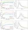 |
Fig. 1 Left panel: time evolution of the disc eccentricity for Kepler-16, Kepler-34 and Kepler-35. Right panel: disc surface density profile at quasi-steady state for the three systems. |
3. Evolution of the binary-disc system
3.1. Evolution of the disc eccentricity
Before presenting simulations of the evolution of embedded circumbinary planets, we first examine briefly the evolution of the binary-disc system and the growth of disc eccentricity. This is not intended to be an exhaustive analysis of this issue as our primary concern in this paper is the evolution of circumbinary planets. We will present a more detailed analysis of the evolution of circumbinary discs in a future publication, where we will consider the influence of radiative processes, self-gravity, binary mass ratios and binary eccentricities.
The left panel of Fig. 1 shows the time evolution of the disc eccentricity ed for the three systems, where ed is defined as (Pierens & Nelson 2007):  (1)In the previous equation, ec is the eccentricity of a fluid element computed at the centre of each grid cell and dS the surface area of one grid cell. For each run, the disc eccentricity initially increases and then reaches a saturated value once viscous damping equilibrates the eccentricity forcing rate due to the binary. The observed oscillations in the disc eccentricity arise because the binary longitude of pericentre maintains a constant value while the disc librates with a libration amplitude of ~108 degrees. This is illustrated in Fig. 2 which shows the time evolution of the disc longitude of pericentre ωd for the Kepler-16 run with α = 10-3 and h = 0.05, where ωd is defined by:
  (2)ωc is the longitude of pericentre of a fluid element evaluated at the centre of each grid cell. The fact that the eccentricity oscillation amplitudes are higher in models with h = 0.07 is likely due to pressure effects which tend to reduce the prograde precession rate of the disc.
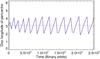 |
Fig. 2 Time evolution of the disc longitude of pericentre for the disc model with h = 0.05 and α = 10-3. The dashed line corresponds to the longitude of pericentre of the binary. |
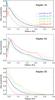 |
Fig. 3 Radial distribution of disc eccentricity for the Kepler-16, Kepler-34 and Kepler-35 runs |
We observe a clear tendency for the final value of ed to increase with increasing h. The Kepler-34 run with h = 0.03 is the one anomaly, which can perhaps be explained by the smaller viscous stress leading to weaker damping of the locally generated eccentricity at large radius. We leave further investigation of this issue for the future publication mentioned at the beginning of this section.
Comparing the upper and lower panels of Fig. 1 for Kepler-16 and Kepler-35, where the binaries have similar eccentricities but different mass ratios, reveals that the saturated value of the disc eccentricity is almost independent of the binary mass ratio. For example, for our fiducial disc model with h = 0.05 and α = 10-3, the steady state value for the disc eccentricity is ed ~ 0.55 in the Kepler-16 run while ed ~ 0.5 for Kepler-35. Comparing the middle and lower panels for Kepler-34 and Kepler-35, however, where the binaries have similar values for qb but very different eccentricities, demonstrates that the final value for ed strongly depends on the binary eccentricity. Not surprisingly, it is found to be higher in Kepler-34 runs with, for example, a stationary value of ed ~ 0.11 reached in the fiducial run with h = 0.05 and α = 10-3. Given that the value for the disc eccentricity is closely related to the size of the inner cavity, as we will see shortly, this is in good agreement with the results of Artymowicz & Lubow (1994) which suggest that the gap size is strongly dependent on the binary eccentricity but depends weakly on the binary mass ratio.
An issue that needs to be investigated is how the final value for the disc eccentricity compares with the expected forced eccentricity resulting from the secular interaction with the binary. The forced eccentricity ef at radius R is given by (Moriwaki & Nakagawa 2004): 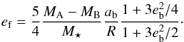 (3)For the Kepler-16 system, this gives ef ~ 0.02 at 1 AU while for Kepler-34 and Kepler-35 which have mass ratios close to unity, the forced eccentricity is much lower (ef ~ 10-3 at 1 AU). Except for the Kepler-16 run with h = 0.03 and α = 10-3, it therefore appears that the saturated value for ed is generally much higher than the forced eccentricity, which is in good agreement with the results of Pelupessy & Portegies Zwart (2013). This indicates that the contribution to the disc eccentricity growth from secular interaction is minimal.
The right panel of Fig. 1 displays the steady-state disc surface density profile for all calculations, time-averaged over 3 × 10³ binary orbits. As the values for h and α are decreased the inner cavity deepens and the cavity edge steepens. Not surprisingly there also appears a general trend for the location of the density peak Rgap to scale with the disc eccentricity. Here, we find that Rgap can be reasonably well approximated by the following fitting relation:  (4)
(4)
3.2. Origin of the disc eccentricity
Previous studies of circumbinary discs (e.g. Papaloizou et al. 2001; Pierens & Nelson 2007) have shown that interaction with the binary can cause the disc to become eccentric. As we have discussed above, the forced eccentricity of the disc due to secular interaction with the binary should be small. For a circular binary, Papaloizou et al. (2001) have shown that the origin of the disc eccentricity involves a parametric instability that causes a spiral wave to be launched at the 3:1 eccentric Lindblad resonance. This instability is generated by non-linear mode coupling between an initial m = 1 eccentric disturbance in the disc and the m = 1 component of the binary potential. This produces a m = 2 wave with pattern speed Ωb / 2 that is launched at the 3:1 Lindblad resonance. The wave transports angular momentum outward, causing the growth of disc eccentricity (Papaloizou et al. 2001). The mechanism at play is very similar to that described by Lubow (1991) in application to superhump phenomena in close binary systems where the disc orbits one component of the binary system. In this case a small binary mass ratio (qb ~ 0.1) allows the 1:3 Lindblad resonance to be present in the disc, leading to the growth of disc eccentricity through a similar instability.
To explore the origin of the disc eccentricity observed in Figs. 1 and 3 we have conducted a number of test calculations. The aim of this study is simply to explore the primary influences on the growth of the eccentricity. In a future paper we will provide an in-depth analysis of disc eccentricity growth in circumbinary systems. The findings of our modest present study may be summarised as follows:
-
Simulations of circumbinary discs with binary mass ratios equal to those in the Kepler-16 and 35 systems typically show the growth of substantial disc eccentricity when the binary eccentricity is set to zero. This clearly demonstrates that non-linear mode coupling and the 3:1 Lindblad resonance play an important role.
-
Simulations were performed for circular binary systems where the inner boundary of the computational domain was placed outside the location of the 3:1 resonance. Disc eccentricity growth was not observed in these cases, confirming the conclusion in the previous paragraph.
-
Simulations were performed for binary systems similar to Kepler-34 with the inner boundary of the computational domain placed between the locations of the 3:1 and 4:1 Lindblad resonance. Strong disc eccentricity growth was observed in this case, suggesting that non-linear mode coupling involving higher-order terms in the potential of the binary also cause the growth of disc eccentricity, at least for the highly eccentric Kepler-34 binary system.
-
(i)
We first considered the case of a fully-formed planet for whichthe planet mass is set to the observed value. For Kepler-16b, thiscorresponds to a mass ratioq = 3.7 × 10⁻⁴, and for Kepler-34b and Kepler-35b q = 1.1 × 10⁻⁴ and q = 7.5 × 10⁻⁵, respectively (see Table 1).
-
(ii)
We then performed a series of simulations in which the planet mass ratio is q = 3 × 10⁻⁵. In that case, the interaction with the disc is linear and we expect the planet to undergo Type I migration. A typical observed evolution outcome of such simulations is stopping of inward migration close to the tidally truncated cavity. Once the planet has reached a quasi-stationary orbit, we allow gas accretion onto the core and examine whether such a scenario can reasonably reproduce the observed systems. Removal of the gas disc occurs in these simulations to mimick photoevaporation on a specified time scale.
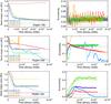 |
Fig. 4 Left panel: time evolution of the semi-major axis of an embedded planet with, from top to bottom, mass ratio corresponding to that of Kepler-16b, Kepler-34b and Kepler-35b. Right panel: time evolution of the eccentricity. For each parameter, the dashed line correspond to the observed value. |
4. Evolution of fully-formed planets
Here we examine the orbital evolution of embedded planets with masses corresponding to the observed values for the three systems Kepler-16, Kepler-34 and Kepler-35. The aim is to investigate how the evolution depends on the employed disc model, and whether or not decent agreement with the observed planet parameters can be obtained.
4.1. Kepler-16b
For our different isothermal disc models, the orbital evolution of an embedded planet with mass ratio corresponding to that of Kepler-16b (q = 3.7 × 10⁻⁴) is presented in the upper panel of Fig. 4. Using the gap opening criteria of Crida et al. (2006) which predicts that gap opening should occur provided that 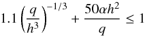 (5)we expect an embedded circumbinary planet with mass ratio q = 3.7 × 10⁻⁴ to significantly perturb the underlying surface density profile in the discs with h = 0.03, h = 0.05 and α ≤ 10-3. This is illustrated in the upper panel of Fig. 5 which displays the disc surface density profile at t = 4 × 10⁴ orbits for all disc models. Gap formation is clearly apparent in the case with h = 0.03, leading also to a substantial increase of the surface density in the inner disc. This results in a strong positive torque being exerted by the inner disc on the planet that prevents inward migration. This result is robust against the choice of inner boundary condition as we performed a simulation using a viscous outflow condition (see Pierens & Nelson 2008a,b) and found no differences.
For disc models with h ≥ 0.05, early evolution typically involves rapid inward migration due to the high surface density at the outer edge of the tidally truncated cavity. At later times the migration rate decreases as the planet enters the cavity and evolves in a region where the surface density gradient is positive. During the run with α = 10-2 and h = 0.05 inward migration stops with the planet settling into an orbit with eccentricity ep ~ 0.04. Migration appears to stop due to the development of a strong positive corotation torque which counterbalances the Lindblad torque within the inner cavity where the surface density has a positive gradient (Masset et al. 2006a), as illustrated in the upper panel of Fig. 5. Saturation of the corotation torque can be prevented provided the viscous time scale across the horseshoe region  , where xs is the half-width of the horseshoe region, is smaller than the horseshoe libration time scale τlib ~ 8πap / (3Ωpxs). Equating these time scales yields an estimate of the minimum value for the viscous stress parameter, α, required to avoid corotation torque saturation. We find:
 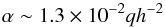 (6)where we have used the fact that for q > 10-4, the half-width of the horseshoe region is xs ~ RH (Masset et al. 2006b). For h = 0.05 this gives α ~ 2 × 10⁻³, indicating that the corotation torque is indeed unsaturated for this model. To clearly demonstrate that this effect is at work here, we have followed the approach of Pierens & Nelson (2007) and computed semi-analytically the torques experienced by the planet using the formulae in Paardekooper et al. (2011). The corotation, Lindblad and total torques exerted on the planet for the three models with h ≥ 0.05 and α ≥ 10-3 are presented as a function of the orbital radius in the lower panel of Fig. 5. Only in the model with h = 0.05 and α = 10-2 is the corotation torque seen to be larger than the Lindblad torque inside the cavity, giving rise to the location R ~ 1 AU where the total torque cancels. Such a value is consistent with the simulation result that migration stops at R ~ 0.82 AU.
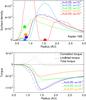 |
Fig. 5 Upper panel: surface density profile at t = 4 × 10⁴ binary orbits for the Kepler-16b runs. Lower panel: semi-analytical torques exerted on Kepler-16b as a function of the orbital radius. |
For the two models with h = 0.05, h = 0.07 and α = 10-3 the corotation torque is much more saturated and the planet is expected to migrate inward further. Consistent with this prediction, the planet is observed to migrate all the way into the inner cavity in the simulation with h = 0.07. Due to the very long run times required by the simulations, the evolution outcome remains uncertain but the fact that there is a significant amount of gas within the cavity for this disc model (see upper right panel of Fig. 1) suggests that inward migration may proceed until the planet enters the region of dynamical instability located at R ≤ 0.64 AU. Extrapolating the observed migration rate forward in time, we estimate that the planet will migrate from R = 0.83 AU to R = 0.64 AU in ~2 × 10⁴ yr, which is much smaller than the disc life time. An alternative outcome, however, may be capture in a mean motion resonance with the binary before dynamical instability occurs.
Contrary to the above prediction concerning saturation of the corotation torque, the run with h = 0.05 and α = 10-3 shows stalling of inward migration from t ~ 4 × 10⁴ P. This stalling does not arise because of a strong positive corotation torque, but rather because migration and gap formation by the planet, combined with tidal truncation by the binary, cause the disc material sitting between the planet and cavity to form a narrow ring. This increases the local surface density in the ring, giving a stronger positive contribution to the Lindblad torque experienced by the planet. This is illustrated in Fig. 6 which shows the evolution of the total torque experienced by the planet, and the contributions from the disc lying interior and exterior to the planet semi-major axis. As time proceeds the amplitude of the (positive) inner-disc torque increases while the (negative) outer-disc torque weakens and the planet halts when the inner and outer torque are in balance.
For the disc model with h = 0.05 and α = 10-4, a similar process does not occur simply because the inner cavity is much deeper in that case. As can be shown in the upper panel of Fig. 5, the inner disc is completely depleted and the evolution outcome appears to be inward migration until the amount of local gas in the cavity becomes too small to make the planet migrate further in. For this model we have performed a long term evolution run for ~1.5 × 10⁵ P and the results are presented in Fig. 7. At t ~ 105 P, we see that inward migration is temporarily halted as the planet reaches ap ~ 0.74 AU. This corresponds to the location of the 6:1 resonance with the binary. From this time the planet evolves for ~5 × 10⁴ binary orbits without migrating just outside the 6:1 resonance with its eccentricity oscillating between 0.007 ≤ ep ≤ 0.1. At t ~ 1.4 × 10⁵ P the planet migrates inward through the 6:1 resonance and halts at semi-major axis close to the currently observed value (ap ~ 0.7 AU). At the end of the simulation, the planet eccentricity oscillates between 0.005 ≤ ep ≤ 0.07, while Kepler data gives ep ~ 0.0069.
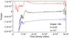 |
Fig. 6 Time evolution of the inner (red), outer (blue) and total (black) torque exerted on Kepler-16b for a disc model with h = 0.05 and α = 10-4. |
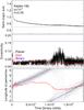 |
Fig. 7 Upper panel: time evolution of the planet semi-major-axis for the Kepler-16b run with α = 10-4 and h = 0.05. Middle panel: time evolution of the planet and disc eccentricities. Lower panel: time evolution of the planet and disc longitudes of pericentre. |
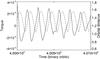 |
Fig. 8 Evolution of the orbital radius (dashed line) of Kepler-34b and evolution of the specific torque (solid line) experienced by the planet over ~5 orbital periods for the run with h = 0.05 and α = 10-2. |
4.2. Kepler-34b
The middle panel of Fig. 4 shows the temporal evolution of the semi-major axis and eccentricity of a planet with q ~ 1.1 × 10⁻⁴, the mass ratio reported for Kepler-34b. Equation (5) suggests that a shallow gap can be formed in the calculation with h = 0.03, and in the one with h = 0.05 and α = 10-4. Significant gap formation is not expected in the other runs.
The evolution is found to be unstable in the simulation with h = 0.07, with the planet experiencing a close encounter with the central binary at t ~ 1.5 × 10⁴ P. This is likely to arise because the disc is highly eccentric (as indicated by the left middle panel of Fig. 1), which drives a large planet eccentricity.
During the runs with h = 0.05 and α ≥ 10-3 the planet migrates inward until the eccentricity increases to ep ~ h, at which point migration stalls due to torque reversal. A planet on a significantly eccentric orbit has smaller angular velocity at apocentre than neighbouring disc material, resulting in the outer disc exerting a positive torque on the planet. The opposite happens at pericentre and the inner disc exerts a negative torque. In general the total orbit-averaged torque experienced by a planet is expected to go from having negative to positive values as the eccentricity grows above values ep > h (Papaloizou & Larwood 2000). For a single planet embedded in a disc this does not normally imply that migration changes from being inward to outward because energy loss associated with eccentricity damping still causes the semi-major axis to decrease, albeit more slowly than for a circular orbit (Cresswell et al. 2007). When the eccentricity is maintained through interaction with the central binary, however, then the total time averaged torque can equal zero and inward migration can be halted. In order to demonstrate that this effect is at work we follow Pierens & Nelson (2008a,b) and plot the disc torque and the planet orbital position over a few planet orbital periods for the run with α = 10-2 in Fig. 8. As expected, the torque exerted on the planet is positive (resp. negative) when the planet is at apocentre (resp. pericentre) and the orbit-averaged torque almost cancels. As noted by Pierens & Nelson (2008a,b), the slight phase shift between the two curves is due to the time needed for the planet to create an inner (outer) wake at apocentre (pericentre). While Kepler-34b is observed to orbit at ap ~ 1.1 AU from the central binary, we note that the final planet semi-major axis in the run with h = 0.05 and α = 10-3 is ap ~ 1.45 AU whereas it is ap ~ 1.3 AU in the calculation with α = 10-2. Interestingly, the final value for the eccentricity ep ~ 0.2 obtained in both runs is rather close from the observed value (ep ~ 0.18).
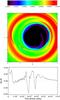 |
Fig. 9 Upper panel: snapshot of the disc surface density at t = for the Kepler-34b run with α = 10-4 and h = 0.05. Lower panel: time evolution for the change of the planet eccentricity induced by the disc. |
For the two runs with (h = 0.03, α = 10-3) and (h = 0.05, α = 10-4) early evolution proceeds similarly, with the planet migrating inward until its eccentricity has increased to a value of ep ~ 0.2, at which point migration stops. As mentioned above, however, the planet can significantly perturb the disc surface density profile in these two cases and this causes the planet to migrate inward at later times because the balance of torques is modified. In both cases the planet migrates inward again from t ~ 1.5 × 10⁴ binary orbits but the final outcome of each run differs. In the h = 0.03 run the planet eccentricity decreases somewhat as the planet migrates deep inside the truncated cavity. Continuation of the run until ~1.5 × 10⁵ binary orbits shows that migration eventually halts when the total orbit-averaged torque vanishes due to the finite eccentricity (see discussion above). At the end of the run the planet semi-major axis reaches a constant value ap ~ 1.35 AU and the eccentricity ep ~ 0.1, much smaller than the observed eccentricity of Kepler-34b. In the simulation with h = 0.05 and α = 10-4 significant growth of the planet eccentricity occurs at t ~ 2.5 × 10⁴ binary orbits, causing the planet to undergo an episode of outward migration. Analysis of this simulation shows that this sudden growth of ep is caused by interaction between the planet and an arc-shaped high density structure related to the m = 1 eccentric mode in the disc, with pattern speed of ~2 × 10³ binary orbits. This is illustrated in the upper panel of Fig. 9 which shows a snapshot of the disc surface density at t ~ 2.5 × 10⁴ binary orbits. In the lower panel of Fig. 9, we plot the temporal evolution of the theoretical change of the planet eccentricity ėp due to the disc with (e.g. Bitsch & Kley 2010): 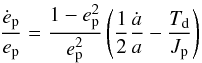 (7)where ȧ is the estimated planet orbital decay rate, Td is the torque exerted by the disc on the planet and Jp is the angular momentum of the planet. This figure clearly demonstrates that the disc is responsible for driving the planet eccentricity upward at t ~ 2.5 × 10⁴. At later times it appears that the combined effect of eccentricity growth and outward migration cause the planet to be in contact with the disc density bump located at ~1.8 AU (see upper panel of Fig. 9), corresponding to material with higher specific angular momentum than the planet. Strong damping of the planet eccentricity occurs at t ~ 2.7 × 10⁴ and the planet migrates inward again. The long-term trend is of decreasing semi-major axis and eccentricity until the torque on the planet becomes negligible. At t ~ 6 × 10⁴ binary orbits the planet semi-major axis is ap ~ 1 AU and its eccentricity has reached a quasi-stationary value of ep ~ 0.03, much smaller than the observed value (ep ~ 0.18). The low value for ep arises because the planet orbits deep inside the tidally-truncated cavity where interaction with the eccentric disc is small. It is also related to the fact that qb ~ 1 for Kepler-34, so that the forced eccentricity due to interaction with the binary is small. Continuation of this run for ~1.5 × 10⁵ binary orbits confirms that the planet migrates very slowly into the gas depleted cavity on a near-circular orbit, but too close to the central binary to be consistent with the observed orbital parameters of Kepler-34b. At t ~ 1.5 × 10⁵ binary orbits, the planet semi-major axis is ap ~ 0.95 AU but there remains evidence that inward migration has not stalled completely.
4.3. Kepler-35b
The orbital evolution of the Kepler-35b simulations are shown for the different disc models in the lower panel of Fig. 4. Compared with Kepler-34b, for which q ~ 1.1 × 10⁴, the mass ratio of Kepler-35b is q ~ 7.5 × 10⁻⁵. Despite the lower binary eccentricity the results for this system look rather similar to the corresponding Kepler-34b runs.
For disc models with h ≥ 0.05 and α ≥ 10-3 the evolution outcomes are stalling of inward migration leaving the planet on an eccentric orbit at fixed semi-major axis. As we have seen in the previous section, this quasi-equilibrium state is reached when the large positive torque experienced by the planet at apocentre is in exact balance with the weaker negative torque felt by the planet at pericentre. The final position of the planet is clearly correlated with the size of the tidally truncated inner cavity. For example, in the run with h = 0.07 and α = 10-3, the density peak is located at R ~ 1.3 AU (see lower right panel of Fig. 1) and the final planet semi-major axis is ap ~ 1.25 AU whereas in the simulation with h = 0.05 and α = 10-3, the density peak is at R ~ 1 AU and migration stops at ap ~ 0.9 AU. Not surprisingly, the final value for the planet eccentricity appears to scale with the disc eccentricity. For instance, in the run with h = 0.05 and α = 10-3, the disc eccentricity is ed ~ 0.05 (see left panel of Fig. 1) and the final ep ~ 0.11. In the run with α = 10-2, the disc eccentricity ed ~ 0.07 and ep ~ 0.21 at the end of the calculation.
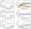 |
Fig. 10 Left panel: time evolution of the semi-major axis of an embedded protoplanet with mass ratio q = 3 × 10⁻⁵. Right panel: time evolution of the planet eccentricity. For each parameter, the dashed line correspond to the observed value. |
A similar outcome is observed in the run with h = 0.03. Here the planet migrates rapidly inward at early times until it reaches a stable, non-migrating configuration with ap ~ 0.7 AU and ep ~ 0.06. Although not shown here, analysis of the torque experienced by the planet clearly reveals a positive (resp. negative) disc torque at planet apocentre (resp. pericentre) and a zero time-averaged total torque.
For the simulation with h = 0.05 and α = 10-4 the process described above makes migration stall at t ~ 104 binary orbits once the planet eccentricity has reached ep ~ 0.12 and its semi-major axis ap ~ 1.1 AU. Similarly to the case of Kepler-34b, the planet is found to migrate inward again at later times due to gap formation by the planet. Subsequent evolution again corresponds to the planet migrating deep inside the inner cavity until the local disc mass becomes too small for further substantial migration. Despite a runtime of ~ 1.5 × 10⁵ binary orbits, an equilibrium state was not reached for this case. At the end of the run, the planet semi-major axis is ap ~ 0.69 but inward migration still proceeds. Its eccentricity, however, has reached a constant value of ep ~ 0.01. Again, such a low value for ep with respect to the observed one (ep ~ 0.04) arises because interaction betwen the planet and the eccentric disc is weak inside the cavity, and the binary mass ratio qb ~ 1 for Kepler-35 so the forced eccentricity remains small.
5. Evolution of migrating and accreting protoplanets
We now consider a scenario in which a ~20 M⊕ core forms in the disc at large distance from the central binary and migrates inward via type I migration until it reaches a location where migration halts. For a 20 M⊕ planet and for the fiducial value of the disc aspect ratio h = 0.05, the half-width of the horseshoe region is 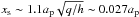 (Paardekooper et al. 2010), which means that at 1 AU (R = 2 in the computational domain), the horseshoe region is resolved by about 5 grid cells in the radial direction. For such a resolution, the relative error on the corotation torque is estimated to be ~15% (Masset 2002). Once migration is stalled, the planet then accretes gas from the disc until the disc has been dispersed by photoevaporation. The primary reason for including photoevaporation is that the planets in the Kepler-16, Kepler-34 and Kepler-35 systems are ~Saturnian mass, and we know from calculations of giant planet formation that such planets are able to accrete gas at very rapid rates (e.g. Pollack et al. 1996). It seems likely that Saturn-mass planets embedded in a substantial reservoir of gas will grow rapidly, so we work with the assumption that growth beyond their observed masses was prevented by removal of the gas disc.
Our procedure is as follows. We first calculate the orbital evolution of protoplanets with mass ratio q = 3 × 10⁻⁵ interacting with the different circumbinary disc models to illustrate the behaviour for different disc parameters. A typical outcome is stopping of inward migration close to the edge of the tidally truncated cavity, and this arises when the planet eccentricity reaches a value ep ~ h. For each of the Kepler binary systems we restart the simulation which uses the disc model that best reproduces the orbital parameters of the observed planet among the simulations presented in Sect. 4, switching on gas accretion onto the core. The final mass and orbital parameters of the planet are set by the gas dispersion time scale.
5.1. Evolution of a protoplanetary core
For the different isothermal disc models we consider, the orbital evolution of an embedded circumbinary protoplanet with mass ratio q = 3 × 10⁻⁵ is presented in Fig. 10. The upper panel shows the results of simulations in which the binary parameters are those of Kepler-16. The middle and lower panels correspond to the Kepler-34 and Kepler-35 systems.
We begin presentation of the simulation results by focusing on these two latter cases, for which similar outcomes are observed. Early evolution typically involves inward migration of the protoplanet and continued growth of its eccentricity due to its interaction with both the central binary and the eccentric disc. At later times inward migration slows down significantly in the run with h = 0.07, and completely stalls or even reverses for thinner disc models. In these cases the final location of the planet is clearly correlated with the position of the gap edge in the right panel of Fig. 1. For example, considering the Kepler-34 system, the density peak is located at R ~ 2 AU in the simulation with h = 0.03 while the middle panel of Fig. 10 shows that migration stops at R ~ 1.8 AU for the same disc model. In the fiducial run with h = 0.05 and α = 10-3, the density peak is located at R ~ 1.5 AU and the planet migrates to ap ~ 1.5 AU before migration halts. We plot both the surface density profile and the planet position at t = 2 × 10⁴ binary orbits in the upper panel of Fig. 11 for this run, showing that the planet halts at the edge of the cavity. As with a number of the simulations described in Sect. 3, the halting of migration occurs because of the torque reversal that occurs when ep ≥ h. For eccentric orbits the corotation torque is expected to be substantially diminished (e.g. Bitsch & Kley 2010), so they cannot be responsible for the halting of migration. Following a strategy similar to that described in Sect. 4.2, where the correlation between the disc torque and the planet orbital radius is examined, we confirm that at late times the planet experiences a positive torque at apocentre and a negative torque at pericentre, leading to a null time-averaged total torque. This is illustrated in the lower panel of Fig. 11 where we plot both the disc torque and the planet orbital position over a few orbital periods of the planet for the run with h = 0.05 and α = 10-3.
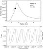 |
Fig. 11 Upper panel: surface density profile and planet position for the Kepler-34 run with h = 0.05 and α = 10-3 at t = 2 × 10⁴ binary orbits. Lower panel: evolution of the orbital radius (dashed line) of a planet with mass ratio q = 3 × 10⁻⁵ and evolution of the specific torque (solid line) experienced by the protoplanet over ~5 orbital periods for the same run. |
The outward migration that we observe in simulations with h ≤ 0.05 and α ≤ 10-3 is likely related to the steepness of the inner cavity edge for these disc models, which combined with the fact that the planet spends more time at apocentre, favours a net positive torque on the planet. In runs with h = 0.07, however, the gradient of surface density in the inner cavity is shallower and so less favourable for stalling or reversing of migration for an eccentric planet. This explains why type I migration is not halted in that case.
The results of the Kepler-16 runs are displayed in the upper panel of Fig. 10. Overall, these are consistent with the corresponding Kepler-34 and Kepler-35 simulations, except for the runs with (h = 0.03, α = 10-3) and (h = 0.05, α = 10-2) in which the final fate of the planet is found to be very different. In the simulation with h = 0.03, migration reverses at ~104 binary orbits due to the eccentric planet orbit, but outward migration accelerates from t ~ 3.5 × 10⁴ binary orbits onward. Inspection of the apsidal lines for both the disc and the planet reveals that from this time these become misaligned, with a tendency for the apsidal line of the disc to slightly lead that of the planet. This promotes outward migration because the planet interacts preferentially with matter whose angular velocity is greater than that of the planet at apocentre (Pierens & Nelson 2008a,b). As outward migration proceeds, the planet eccentricity progressively decreases. Continuation of the run shows that the planet eventually migrates inward again once its semi-major axis has reached ap ~ 1.3 AU. Therefore we can reasonably expect the long term evolution for this run to consist of periods of inward followed by outward migration until disc dispersal.
With respect to the other disc models, the positive gradient of surface density at the inner edge of the tidally truncated cavity is shallower in the simulation with (h = 0.05, α = 10-2) (see upper right panel of Fig. 1). Consequently, torque reversal is not observed in that case and the planet migrates inward continuously. This inward migration is accompanied by significant growth of the planet eccentricity due to its interaction with both the binary and eccentric disc. The eccentricity increases to ep ~ 0.3 at t ~ 4 × 10⁴ P. At t ~ 4.3 × 10⁴ P, the eccentricity growth causes the planet to undergo a close encounter with the binary and to be subsequently ejected from the system.
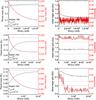 |
Fig. 12 Left panel: time evolution of the planet mass (black) and disc mass (red) for simulations in which a migrating embryo grows by accreting gas material from the disc. Right panel: time evolution of semi-major axis (black) and eccentricity (red). For each parameter, the dashed line correspond to the observed value. |
5.2. Evolution of an accreting core
In this section we use the disc model that best reproduces the observed parameters of each of the three Kepler systems to focus on a more realistic evolution scenario in which a migrating embryo grows by accreting gas from the disc at the same time as the disc is being dispersed. We expect both core growth and inward migration to be terminated as a result of disc clearing, which is thought to be mainly driven by photoevaporation induced by UV irradiation and/or X-rays at late times (Owen et al. 2011). Gas disc dispersal by photoevaporation is modelled in the simplest possible manner by forcing the gas surface density to decay exponentially with an e-folding time tdis, for which we consider values 104 and 105 P. These values are broadly consistent with estimates of the gas dispersal time scale due to UV photoevaporation which give tdis ~ 105 years (Alexander et al. 2006). We also vary the rate at which the planet accretes gas from the disc by choosing different values for the accretion parameter, facc, defined in Sect. 2.2. For each value of disc dispersal time tdis we perform simulations for values of facc = 1, 2, 3, ..., 10. We note that facc = 1 corresponds to the maximally accreting planet (e.g. Kley 1999).
5.2.1. Kepler-16
A core mass of mp ~ 20M⊕ is close to the value required for runaway gas accretion in the core accretion scenario of gas giant planet formation (Pollack et al. 1996; Papaloizou & Nelson 2005), which is why this core mass was chosen for these simulations. The disc model that gave best agreement with the observed orbital parameters of Kepler-16b in Sect. 4.1 had h = 0.05 and α = 10-4, so we consider a model that was run with planetary mass ratio q = 6.7 × 10⁻⁵ (mp ~ 20M⊕) until migration halts, and then restart with gas accretion and photoevaporation switched on for the model parameters described above.
The evolution of the model that best fits the observed Kepler-16b system is shown in the top panels of Fig. 12, and had parameters facc = 1 and tdis = 105 P. The left panel shows the planet and disc masses, and the right panel shows the semi-major axis and eccentricity. The planet mass slightly exceeds the inferred mass of Kepler-16b, the semi-major axis stalls just outside of the observed value, and the eccentricity has a mean value ep ≃ 0.03 (to be compared with the smaller value of 7 × 10⁻³ inferred from observations). It seems very likely that subtle tweaking of the model parameters could lead to a planet whose mass and semi-major axis agrees much more accurately with the observed values, but our aim here is not to obtain perfect agreement with the observed values using a highly-simplified disc model so we do not attempt to refine the values of facc and tdis here. Obtaining a mean eccentricity equal to the very small value reported for this system would appear to present a greater challenge. It remains to be seen whether a more realistic disc model will lead to a smaller final planet eccentricity.
5.2.2. Kepler-34
The simulations in Sect. 4.2 indicate that the disc parameters h = 0.05 and α = 10-2 best produce a final planetary configuration that approximates the observed values. The simulation with planetary mass ratio q = 3 × 10⁻⁵ described in Sect. 5.1 above was restarted with gas accretion and disc dispersal switched on, and the results from the run whose outcome best matches the observed Kepler-34b system are shown in the middle panels of Fig. 12. This simulation adopted facc = 3 and tdis = 104 P. We see that the simulated planet mass undershoots the observed value slightly (a slightly larger value of tdis would presumably improve this). We see that the semi-major axes and eccentricities barely change at all during the time when gas accretion occurs, suggesting that the final orbital configuration obtained for the 20 M⊕ embryo is very similar to that for the final planet after accretion. Inspection of Fig. 4 shows that migration of the fully-formed planet also leads to very similar final values for ap and ep. Unlike in the Kepler-16 run, the simulations of Kepler-34b using the disc model h = 0.05 and α = 10-2 produce the same set of orbital elements when considering a fully-formed planet, a migrating 20 M⊕ core, and a gas-accreting core. Producing a closer approximation to the observed system will therefore require modest tweaking of the disc physics rather than the parameters facc and tdis.
5.2.3. Kepler-35
The disc model with h = 0.03 and α = 10-3 was shown to be the best candidate for reproducing the orbital configuration of Kepler-35b in Sect. 4.3. The simulation with planetary mass ratio q = 3 × 10⁻⁵ described in Sect. 5.1 above was restarted with gas accretion and disc dispersal switched on, and the results from the run whose outcome best matches the observed Kepler-35b system are shown in the lower panels of Fig. 12. This simulation adopted facc = 4 and tdis = 104 P, and produces a planet mass close to the one observed, but a semi-major axis that is larger than the observed value (ap = 0.7 AU versus 0.6 AU). This is consistent with the corresponding run with the fully formed planet in Sect. 4.3 which also resulted in a planet with ap ≃ 0.7. Reducing this value to agree with the observed one will therefore require moderate adjustment of the disc model. The eccentricity evolution results in a final mean value of ep ≃ 0.015. Interestingly this is smaller than the observed value of 0.04, unlike the value obtained from the simulation of the fully-formed planet which resulted in ep ≃ 0.06 (see Fig. 4).
It is clear from this and the other simulations described for Kepler-35b and Kepler-16b that obtaining fits to the observations for all system parameters would require implementation of a multi-dimensional fitting procedure whose complexity would not be justified given the simplicity of our underlying model.
5.3. Validity of the isothermal approximation
In the locally isothermal limit, the only contribution to the corotation torque is the vorticity-related corotation torque which scales with the vortensity (i.e. the ratio between vorticity and surface density) gradient. In the context of circumbinary discs, it has been shown that at the inner edge of the tidally truncated cavity where the surface density has a large positive gradient, the (positive) vorticity-related corotation torque can be strong enough to counterbalance the (negative) differential Lindblad torque, leading to halting of Type I migration (Masset et al. 2006a,b; Pierens & Nelson 2007). This arises provided that the amplitude of the corotation torque is close to its optimal value, which is reached when: i) the viscous diffusion time scales across the horseshoe region are approximately equal to half the libration time scale (Baruteau & Masset 2013); ii) the planet eccentricity ep is significantly smaller than the dimensionless half-width of the horseshoe region  . We expect indeed that when
  , the radial excursion of the planet becomes larger than the half-width of the horseshoe region and consequently the corotation torque to be strongly attenuated (Bitsch & Kley 2010). For ep ~ 0.1, which is a value typical to what is observed in the isothermal simulations of 20M⊕ cores presented above, it is likely that the contribution of the corotation torque to the total torque is relatively weak (see Fig. 2 of Bitsch & Kley 2010).
In non-isothermal discs, the corotation torque consists of the vorticity-related corotation torque plus an additional component which scales with the entropy gradient (Paardekooper & Papaloizou 2008; Baruteau & Masset 2008). For a negative entropy gradient inside the disc, this entropy-related corotation torque is positive and can be responsible for significantly slowing down or even reverse Type I migration. Depending on whether or not a locally isothermal equation of state is used and provided that the amplitude of the corotation torque is close to its fully-unsaturated value, simulations of the evolution of 20M⊕ cores in the Kepler-16, Kepler-34 and Kepler-35 systems may therefore lead to very different outcomes. Regarding the simulations with fully-formed planets, we note that the issue of the equation of state does not really matter since we expect a Saturn-mass planet to open a partial gap in the disc, with the consequence that the corotation torque is weakened (Kley & Crida 2008).
Assuming a 20M⊕ core forming at ≳10 AU (Marzari et al. 2013), namely in a region of small disc eccentricity, its migration can be directed either outward or inward in the non-isothermal case, depending on the level of saturation of the corotation torque. In both cases, however, we expect the protoplanet to reach a zero-migration line where it becomes trapped (Lyra et al. 2010; Hellary & Nelson 2012). As the disc disperses, the zero-migration line is shifted inward with the main consequence that the planet eventually enters a region of high disc eccentricity. In that case, the embryo should decouple from the zero-migration line at a point in time where its eccentricity becomes high enough for the corotation torque to be significantly weakened. The planet then migrates inward again and we expect evolution outcomes rather similar to those arising in isothermal runs. This implies that in the phase after the embryos eccentricities have reached values  , the results of isothermal runs presented above are relatively robust regarding the equation of state.
In disc models with moderate values of disc eccentricity, if any, an alternative outcome is that the planet moves inward as the disc disperses until it reaches the inner edge of the inner cavity where it becomes trapped due to the action of the vorticity-related corotation torque.
As the planet eccentricity is mainly driven by the eccentric disc, this raises the issue of the disc eccentricity in the radiative case. Clearly, this issue needs to be examined in more details and we will address this issue and its consequence on the evolution of protoplanetary cores in the Kepler-16, Kepler-34 and Kepler-35 systems in a future publication.
6. Discussion and conclusion
In this paper, we have presented the results of hydrodynamic simulations that examine the migration and orbital evolution of embedded circumbinary planets orbiting around the three close binary systems Kepler-16, Kepler-34 and Kepler-35. We began our study by examining the evolution of the binary-plus-disc system in the absence of an embedded planet in order to obtain an improved understanding of how circumbinary discs are structured by the central binary as a function of binary and disc parameters. In particular, we examined how the mean surface density radial profile and disc eccentricity vary for the three Kepler binary systems as a function of disc aspect ratio, h, and viscosity parameter α. Our results indicate that for each binary system the disc structure is a sensitive function of the disc parameters, with the tidally trucated cavity displaying significant changes in both radius and internal density structure as a function of h and α. Furthermore, the eccentricity of the disc also shows strong dependence on disc parameters: we observe a general tendency for the disc eccentricity to increase with increasing h, which is likely due to the fact that the eccentricity is more effectively communicated through the disc for larger values of h.
Our investigation confirms that the origin of the disc eccentricity is non-linear mode coupling as described previously for circumbinary and circumstellar discs by Papaloizou et al. (2001) and Lubow (1991), respectively. The forced eccentricity due to secular interaction with the binary is too small to explain the simulations (see Sect. 3.1). The Papaloizou et al. (2001) study indicated that coupling between an initial m = 1 eccentric disc disturbance and the m = 1 component of the binary potential with pattern speed equal to the mean motion of the binary leads to excitation of a wave at the 3:1 eccentric Lindblad resonance which transports angular momentum outward, increasing the disc eccentricity. Our study indicates that the 3:1 resonance is important also for the eccentric Kepler binary systems, but also suggests that mode coupling involving higher order terms in the binary potential may also be important. Given the importance of the disc eccentricity for determining the orbital parameters of embedded circumbinary planets, a further, more in-depth study of circumbinary disc dynamics is certainly warranted.
Our study of the evolution of circumbinary planets embedded in the circumbinary discs described above adopted two basic scenarios. In the first we considered the orbital evolution of a fully-formed planet in a variety of disc models for each binary system, and attempted to determine which of the disc models resulted in planet orbits that best agree with the Kepler observations. The basic mode of evolution in these runs was inward migration of the planet, followed by stalling of migration in the tidally truncated disc cavity. The planetary orbits typically become non-circular due to interaction with the circumbinary disc and binary, with the former effect usually being dominant. In the second, more realistic scenario, we consider the evolution of a low-mass (~20 M⊕) core, which migrates inward until it stalls when it enters the inner disc cavity. Gas accretion onto this core is then initiated, along with dispersal of the gas disc (mimicking photoevaporation for example), until the planet achieves its final mass and orbital configuration. We examine the outcome of this scenario as a function of gas accretion rate onto the planet and disc dispersal time scale, and for each of the Kepler binary systems we form circumbinary planets which are similar to the observed systems. Furthermore, we generally find that for each of the Kepler binary systems the final orbital configuration of the planet is similar, independent of the two migration scenarios adopted (fully-formed planet versus migrating and accreting core).
We find that the simulation that produces the closest approximation to the observed system for each of the Kepler binaries uses a different disc model: no single disc model produces a final planet that is in close agreement with the observational data for all planets. For Kepler-16b, a disc model with h = 0.05 and α = 10-4 produces the best-fit. Good agreement with the observed planet mass and semi-major axis can be obtained, but all models consistently predict a larger eccentricity for the planet than observed (typically ep ≳ 0.03 is obtained, compared with the observed value of 7 × 10⁻³). Given that the eccentric disc is largely responsible for the eccentricity growth, this indicates that a model with smaller disc eccentricity may be required to provide a better fit. For Kepler-34b the disc with h = 0.05 and α = 10-2 best reproduces the orbital parameters of the planet. For this system a plausible model of core formation at large radius followed by inward migration and gas accretion can be constructed that provides a good fit to the planet mass and eccentricity, but none of our simulations were successful in forming a planet whose final semi-major axis is as small as observed (values of ap ≃ 1.3 AU were obtained, to be compared with the observed value of 1.1 AU). The stalling of migration occurs through an interplay between the planetary eccentricity and the surface density profile in the inner cavity, since this is what determines the averaged torque balance. Obtaining the required surface density profile very likely requires a more sophisticated disc model in which either h or α are not constant. For Kepler-35b a disc model with h = 0.03 and α = 10-3 produces the best fit to the planet orbital parameters. A simple model of core migration followed by gas accretion and disc dispersal can form a planet with mass close to the observed value, but in general the semi-major axis stalls at a value that is too large (values of ap ≃ 0.7 AU are obtained, compared with the observed value 0.6 AU). The best-fit migration-plus-accretion model for this system produces an eccentricity that is too small (in stark contrast to the Kepler-16b runs), with a mean value of ep ≃ 0.01 being obtained, versus the observed value of 0.04. Interestingly, the best-fit model for a fully-formed planet that migrates in and stalls produces a value ep ≃ 0.06, so the observed value falls neatly between these two simulated values. Again, it is likely that the details of the disc eccentricity distribution and the surface density profile in the inner disc cavity determine the fine details of the planetary orbital parameters, and obtaining improved fits may simply require a more sophisticated disc model than we have considered.
In summary, our simulation results indicate strongly that the Kepler-16, Kepler-34 and Kepler-35 planets can be explained by a scenario in which a massive rocky/icy core forms at large distance from the central binary in a circumbinary disc and migrates inward until it stalls in the tidally truncated cavity formed by the central binary. Subsequent gas accretion leads to the growth of the planet, and the changing balance of torques leads to a further episode of modest inward migration. We argue that the final configurations of these planets are likely to be determined in part by dispersal of the gas disc, since the observed planets are all expected to be in the regime where runaway gas accretion can occur (e.g. Pollack et al. 1996; Papaloizou & Nelson 2005) – i.e. in the Saturnian or sub-Saturnian mass range.
The models we have presented are in essence the simplest we can compute, so our intention has not been to provide rigorous fits to the observational data. Instead, our aim was to demonstrate the plausibility of the core formation, migration and gas accretion picture for each of the Kepler circumbinary planets. Our simulations demonstrate the importance of the circumbinary disc structure for determining the final parameters of forming circumbinary planets, and it is clear that improved understanding of these systems will require more in-depth modelling that includes radiation transport, self-gravity and additional processes that determine the detailed stucture of the circumbinary disc. These issues will be examined in a future publication.
Acknowledgments
Computer time for this study was provided by the computing facilities MCIA (Mésocentre de Calcul Intensif Aquitain) of the Université de Bordeaux and by HPC resources from GENCI-cines (c2012046957).
References
- Alexander, R. D., Clarke, C. J., & Pringle, J. E. 2006, MNRAS, 369, 229 [NASA ADS] [CrossRef] [Google Scholar]
- Artymowicz, P., & Lubow, S. H. 1994, ApJ, 421, 651 [NASA ADS] [CrossRef] [Google Scholar]
- Baruteau, C., & Masset, F. 2008, ApJ, 672, 1054 [NASA ADS] [CrossRef] [Google Scholar]
- Baruteau, C., & Masset, F. 2013, Lect. Notes Phys. (Berlin: Springer Verlag), 861, 201 [NASA ADS] [CrossRef] [Google Scholar]
- Bell, K. R., & Lin, D. N. C. 1994, ApJ, 427, 987 [NASA ADS] [CrossRef] [Google Scholar]
- Binney, J., & Tremaine, S. 1987, Galactic Dynamics (Princeton, NJ: Princeton University Press), 747 [Google Scholar]
- Bitsch, B., & Kley, W. 2010, A&A, 523, A30 [NASA ADS] [CrossRef] [EDP Sciences] [Google Scholar]
- Cresswell, P., Dirksen, G., Kley, W., & Nelson, R. P. 2007, A&A, 473, 329 [NASA ADS] [CrossRef] [EDP Sciences] [Google Scholar]
- Crida, A., Morbidelli, A., & Masset, F. 2006, Icarus, 181, 587 [Google Scholar]
- Crida, A., Baruteau, C., Kley, W., & Masset, F. 2009, A&A, 502, 679 [NASA ADS] [CrossRef] [EDP Sciences] [Google Scholar]
- de Val-Borro, M., Edgar, R. G., Artymowicz, P., et al. 2006, MNRAS, 370, 529 [NASA ADS] [CrossRef] [Google Scholar]
- Doyle, L. R., Carter, J. A., Fabrycky, D. C., et al. 2011, Science, 333, 1602 [NASA ADS] [CrossRef] [MathSciNet] [PubMed] [Google Scholar]
- Dutrey, A., Guilloteau, S., & Simon, M. 1994, A&A, 286, 149 [NASA ADS] [Google Scholar]
- Günther, R., Schäfer, C., & Kley, W. 2004, A&A, 423, 559 [NASA ADS] [CrossRef] [EDP Sciences] [Google Scholar]
- Hellary, P., & Nelson, R. P. 2012, MNRAS, 419, 2737 [NASA ADS] [CrossRef] [Google Scholar]
- Holman, M. J., & Wiegert, P. A. 1999, AJ, 117, 621 [NASA ADS] [CrossRef] [Google Scholar]
- Hubeny, I. 1990, ApJ, 351, 632 [NASA ADS] [CrossRef] [Google Scholar]
- Kley, W. 1999, MNRAS, 303, 696 [NASA ADS] [CrossRef] [Google Scholar]
- Kley, W., & Nelson, R. P. 2010, Astrophys. Space Sci. Lib., 366, 135 [NASA ADS] [CrossRef] [Google Scholar]
- Lin, D. N. C., & Papaloizou, J. 1986, ApJ, 309, 846 [NASA ADS] [CrossRef] [Google Scholar]
- Lubow, S. H. 1991, ApJ, 381, 259 [NASA ADS] [CrossRef] [Google Scholar]
- Lyra, W., Paardekooper, S.-J., & Mac Low, M.-M. 2010, ApJ, 715, L68 [NASA ADS] [CrossRef] [Google Scholar]
- Masset, F. 2000, A&AS, 141, 165 [NASA ADS] [CrossRef] [EDP Sciences] [Google Scholar]
- Masset, F. S., D’Angelo, G., & Kley, W. 2006a, ApJ, 652, 730 [NASA ADS] [CrossRef] [Google Scholar]
- Masset, F. S., Morbidelli, A., Crida, A., & Ferreira, J. 2006b, ApJ, 642, 478 [NASA ADS] [CrossRef] [Google Scholar]
- Marzari, F., Thébault, P., & Scholl, H. 2008, ApJ, 681, 1599 [NASA ADS] [CrossRef] [Google Scholar]
- Marzari, F., Scholl, H., Thébault, P., & Baruteau, C. 2009, A&A, 508, 1493 [NASA ADS] [CrossRef] [EDP Sciences] [Google Scholar]
- Marzari, F., Baruteau, C., Scholl, H., & Thebault, P. 2012, A&A, 539, A98 [NASA ADS] [CrossRef] [EDP Sciences] [Google Scholar]
- Marzari, F., Thebault, P., Scholl, H., Picogna, G., & Baruteau, C. 2013, A&A, 553, A71 [NASA ADS] [CrossRef] [EDP Sciences] [Google Scholar]
- Meschiari, S. 2012a, ApJ, 752, 71 [NASA ADS] [CrossRef] [Google Scholar]
- Meschiari, S. 2012b, ApJ, 761, L7 [NASA ADS] [CrossRef] [Google Scholar]
- Moriwaki, K., & Nakagawa, Y. 2004, ApJ, 609, 1065 [NASA ADS] [CrossRef] [Google Scholar]
- Nelson, R. P. 2003, MNRAS, 345, 233 [NASA ADS] [CrossRef] [Google Scholar]
- Nelson, R. P., Papaloizou, J. C. B., Masset, F., & Kley, W. 2000, MNRAS, 318, 18 [NASA ADS] [CrossRef] [Google Scholar]
- Orosz, J. A., Welsh, W. F., Carter, J. A., et al. 2012a, ApJ, 758, 87 [NASA ADS] [CrossRef] [Google Scholar]
- Orosz, J. A., Welsh, W. F., Carter, J. A., et al. 2012b, Science, 337, 1511 [NASA ADS] [CrossRef] [PubMed] [Google Scholar]
- Owen, J. E., Ercolano, B., & Clarke, C. J. 2011, MNRAS, 412, 13 [NASA ADS] [CrossRef] [Google Scholar]
- Paardekooper, S.-J., & Papaloizou, J. C. B. 2008, A&A, 485, 877 [NASA ADS] [CrossRef] [EDP Sciences] [Google Scholar]
- Paardekooper, S.-J., Baruteau, C., Crida, A., & Kley, W. 2010, MNRAS, 401, 1950 [NASA ADS] [CrossRef] [Google Scholar]
- Paardekooper, S.-J., Baruteau, C., & Kley, W. 2011, MNRAS, 410, 293 [NASA ADS] [CrossRef] [Google Scholar]
- Paardekooper, S.-J., Leinhardt, Z. M., Thébault, P., & Baruteau, C. 2012, ApJ, 754, L16 [NASA ADS] [CrossRef] [Google Scholar]
- Papaloizou, J. C. B., & Larwood, J. D. 2000, MNRAS, 315, 823 [NASA ADS] [CrossRef] [Google Scholar]
- Papaloizou, J. C. B., & Nelson, R. P. 2005, A&A, 433, 247 [NASA ADS] [CrossRef] [EDP Sciences] [Google Scholar]
- Papaloizou, J. C. B., Nelson, R. P., & Masset, F. 2001, A&A, 366, 263 [NASA ADS] [CrossRef] [EDP Sciences] [Google Scholar]
- Pelupessy, F. I., & Portegies Zwart, S. 2013, MNRAS, 429, 895 [NASA ADS] [CrossRef] [Google Scholar]
- Pierens, A., & Nelson, R. P. 2007, A&A, 472, 993 [NASA ADS] [CrossRef] [EDP Sciences] [Google Scholar]
- Pierens, A., & Nelson, R. P. 2008a, A&A, 478, 939 [NASA ADS] [CrossRef] [EDP Sciences] [Google Scholar]
- Pierens, A., & Nelson, R. P. 2008b, A&A, 483, 633 [NASA ADS] [CrossRef] [EDP Sciences] [Google Scholar]
- Pollack, J. B., Hubickyj, O., Bodenheimer, P., et al. 1996, Icarus, 124, 62 [NASA ADS] [CrossRef] [Google Scholar]
- Press, W. H., Teukolsky, S. A., Vetterling, W. T., & Flannery, B. P. 1992, Numerical Recipes in C: The Art of Scientific Computing, 2nd edn. (Cambridge: University Press) [Google Scholar]
- Scholl, H., Marzari, F., & Thébault, P. 2007, MNRAS, 380, 1119 [NASA ADS] [CrossRef] [Google Scholar]
- Schwamb, M. E., Orosz, J. A., Carter, J. A., et al. 2013, ApJ, 768, 127 [NASA ADS] [CrossRef] [Google Scholar]
- Shakura, N. I., & Sunyaev, R. A. 1973, A&A, 24, 337 [NASA ADS] [Google Scholar]
- Tanaka, H., Takeuchi, T., & Ward, W. R. 2002, ApJ, 565, 1257 [NASA ADS] [CrossRef] [Google Scholar]
- van Leer, B. 1977, J. Computat. Phys., 23, 276 [NASA ADS] [CrossRef] [Google Scholar]
- Ward, W. R. 1997, Icarus, 126, 261 [NASA ADS] [CrossRef] [Google Scholar]
- Welsh, W. F., Orosz, J. A., Carter, J. A., et al. 2012, Nature, 481, 475 [NASA ADS] [CrossRef] [PubMed] [Google Scholar]
- Winn, J. N., Albrecht, S., Johnson, J. A., et al. 2011, ApJ, 741, L1 [NASA ADS] [CrossRef] [Google Scholar]
All Tables
All Figures
|
Fig. 1 Left panel: time evolution of the disc eccentricity for Kepler-16, Kepler-34 and Kepler-35. Right panel: disc surface density profile at quasi-steady state for the three systems. |
| In the text | |
|
Fig. 2 Time evolution of the disc longitude of pericentre for the disc model with h = 0.05 and α = 10-3. The dashed line corresponds to the longitude of pericentre of the binary. |
| In the text | |
|
Fig. 3 Radial distribution of disc eccentricity for the Kepler-16, Kepler-34 and Kepler-35 runs |
| In the text | |
|
Fig. 4 Left panel: time evolution of the semi-major axis of an embedded planet with, from top to bottom, mass ratio corresponding to that of Kepler-16b, Kepler-34b and Kepler-35b. Right panel: time evolution of the eccentricity. For each parameter, the dashed line correspond to the observed value. |
| In the text | |
|
Fig. 5 Upper panel: surface density profile at t = 4 × 10⁴ binary orbits for the Kepler-16b runs. Lower panel: semi-analytical torques exerted on Kepler-16b as a function of the orbital radius. |
| In the text | |
|
Fig. 6 Time evolution of the inner (red), outer (blue) and total (black) torque exerted on Kepler-16b for a disc model with h = 0.05 and α = 10-4. |
| In the text | |
|
Fig. 7 Upper panel: time evolution of the planet semi-major-axis for the Kepler-16b run with α = 10-4 and h = 0.05. Middle panel: time evolution of the planet and disc eccentricities. Lower panel: time evolution of the planet and disc longitudes of pericentre. |
| In the text | |
|
Fig. 8 Evolution of the orbital radius (dashed line) of Kepler-34b and evolution of the specific torque (solid line) experienced by the planet over ~5 orbital periods for the run with h = 0.05 and α = 10-2. |
| In the text | |
|
Fig. 9 Upper panel: snapshot of the disc surface density at t = for the Kepler-34b run with α = 10-4 and h = 0.05. Lower panel: time evolution for the change of the planet eccentricity induced by the disc. |
| In the text | |
|
Fig. 10 Left panel: time evolution of the semi-major axis of an embedded protoplanet with mass ratio q = 3 × 10⁻⁵. Right panel: time evolution of the planet eccentricity. For each parameter, the dashed line correspond to the observed value. |
| In the text | |
|
Fig. 11 Upper panel: surface density profile and planet position for the Kepler-34 run with h = 0.05 and α = 10-3 at t = 2 × 10⁴ binary orbits. Lower panel: evolution of the orbital radius (dashed line) of a planet with mass ratio q = 3 × 10⁻⁵ and evolution of the specific torque (solid line) experienced by the protoplanet over ~5 orbital periods for the same run. |
| In the text | |
|
Fig. 12 Left panel: time evolution of the planet mass (black) and disc mass (red) for simulations in which a migrating embryo grows by accreting gas material from the disc. Right panel: time evolution of semi-major axis (black) and eccentricity (red). For each parameter, the dashed line correspond to the observed value. |
| In the text | |
Current usage metrics show cumulative count of Article Views (full-text article views including HTML views, PDF and ePub downloads, according to the available data) and Abstracts Views on Vision4Press platform.
Data correspond to usage on the plateform after 2015. The current usage metrics is available 48-96 hours after online publication and is updated daily on week days.
Initial download of the metrics may take a while.