| Issue |
A&A
Volume 556, August 2013
|
|
|---|---|---|
| Article Number | A81 | |
| Number of page(s) | 7 | |
| Section | Interstellar and circumstellar matter | |
| DOI | https://doi.org/10.1051/0004-6361/201220419 | |
| Published online | 31 July 2013 | |
A representative sample of Be stars
V. Hα variability⋆
Astrophysics Research Institute, Liverpool John Moores University, Twelve Quays House, Birkenhead CH41 1LD, UK
e-mail: This email address is being protected from spambots. You need JavaScript enabled to view it.
Received: 20 September 2012
Accepted: 9 May 2013
Abstract
Aims. We attempt to determine if a dependency on spectral subtype or vsin i exists for stars undergoing phase-changes between B and Be states, as well as for those stars exhibiting variability in Hα emission.
Methods. We analysed the changes in Hα line strength for a sample of 55 Be stars of varying spectral types and luminosity classes using five epochs of observations taken over a ten year period between 1998 and 2010.
Results. We find i) that the typical timescale between which full phase transitions occur is most likely of the order of centuries, although no dependency on spectral subtype or vsin i could be determined due to the low frequency of phase-changing events observed in our sample; ii) that stars with earlier spectral types and larger values of vsin i show a greater degree of variability in Hα emission over the timescales probed in this study; and iii) a trend of increasing variability between the shortest and longest baselines for stars of later spectral types and with smaller values of vsin i.
Key words: stars: emission-line, Be / circumstellar matter
Table 1 is available in electronic form at http://www.aanda.org
© ESO, 2013
1. Introduction
The emission lines displayed by Be stars are known to be transient (Kogure 1990), with emission varying over timescales ranging from less than a day (Percy et al. 2002) to years (Miroshnichenko et al. 2002). This emission variability is reflected in the first working definition given by Collins (1987) who defined a Be star as “a non-supergiant B star whose spectrum has, or had at some time, one or more Balmer lines in emission”.
More recently, this definition has had to be refined to exclude emission-line stars whose disk formation mechanisms were accretion, e.g. Herbig AeBe stars. Consequently, a new subgroup of these emission-line stars, termed “classical Be stars”, was created. Classical Be stars are characterised by their rapid rotation and decretion disks (see Porter & Rivinius 2003). Martayan et al. (2011) proposed a refinement of Collins’ definition to “... a star with innate or acquired very fast rotation which combined to other mechanisms ... leads to episodic matter ejections creating a circumstellar decretion disk or envelope” to not only reflect the larger range of spectral types over which the phenomena have been observed to occur (Conti & Leep 1974; Rauw et al. 2007) albeit with lesser frequency (Negueruela et al. 2004), but also to constrain the method whereby the disk is formed. It is these classical Be stars that are the subject of the following study.
In 1999, a multiwavelength survey of a representative sample of 58 Be stars was undertaken (Steele et al. 1999; Clark & Steele 2000; Steele & Clark 2001; Howells et al. 2001). The sample is “representative” in that it attempted to include objects of each spectral type and luminosity class and so does not serve to reflect the spectral type or luminosity class distribution of Be stars.
One of the conclusions drawn from this survey was that at the time of observation, non-emission line stars in the sample (i.e. by definition, ones that must have shown emission in the past) had lower rotational velocities and earlier spectral types, an implication being that they may be more prone to B/Be phase changes (Steele & Clark 2001). Using optical spectrographic follow up taken ten years after the sample was first observed, the validity of these statements will be investigated further in this paper.
2. Observations and data reduction
The targets observed were taken from Steele et al. (1999, hereafter S99). The catalogue names of the targets and some of their fundamental properties (viz. spectral class, luminosity class, V band mag., vsin i) are shown in Table 1.
In S99, the stars were reclassified under the MK scheme (Morgan & Keenan 1973) using spectra taken by the Intermediate Dispersion Spectrograph (IDS) on the Isaac Newton Telescope (INT), rather than relying on values taken from the literature. Rotational velocities were also determined in S99 by fitting Gaussian profiles to 4 HeI lines at 4026 Å, 4143 Å, 4387 Å and 4471 Å and applying the full width half maximum – vsin i correlation of Slettebak et al. (1975). It should be noted that this method of inferring a vsin i has not taken into account the effect of gravity darkening, which has been shown to introduce a redundancy between line profile width and vsin i at the largest rotation speeds (Townsend et al. 2004; Frémat et al. 2005), leading to underestimates of the true rotation speed for the fastest rotators. Residual emission within the HeI lines may have also introduced a bias towards lower vsin i for earlier subtypes.
Five epochs of observations were used in the following analysis (hereafter referred to as the INT, F1, F2, F3 and F4 datasets) and were obtained using both the IDS and FRODOSpec (Morales-Rueda et al. 2004) on the Liverpool Telescope (Steele et al. 2004).
The IDS observations used in this analysis were made on the night of 1998 August 3 using the R1200Y grating with a slit width of 1.15 arcsec, corresponding to a dispersion of ~0.5 Å/pixel on the EEV12 CCD. A central wavelength of 6560 Å was chosen, giving a wavelength range between 5800−7100 Å.
Reduction of INT data was performed using Figaro according to the standard prescription for long-slit spectra. Tungsten lamp flats were used to map the slit response and sky flats the pixel-to-pixel flat field variations. Target spectra were extracted using simple extraction and a sky region of the same size was also extracted and subtracted from each target spectrum. To wavelength calibrate the target frames, arc exposures were taken at the start, middle and end of the night using CuAr and CuNe lamps. After extracting their spectra, the calibrations were determined and copied onto the target spectra.
All FRODOSpec observations were taken over a period between September 2009 and November 2010. Observations for the F1 dataset were made between 08/09/2009 and 26/09/2009, F2 between 03/11/2009 and 26/12/2009, F3 between 18/07/2010 and 29/08/2010 and F4 between 10/10/2010 and 23/11/2010.
The first two epochs of data, F1 and F2, were taken using the red diffraction gratings. The last two, F3 and F4, were taken using the higher resolution red VPH gratings. FRODOSpec provides wavelength coverage from 3900−5700 Å (blue arm) and 5800−9400 Å (red arm) for the lower resolution configuration (R = 2600 and 2200 respectively) and 3900−5100 Å (blue arm) and 5900−8000 Å (red arm) for the higher resolution (R = 5500 and 5300 respectively). FRODOSpec reduction was performed using the pipeline discussed in Barnsley et al. (2012).
3. Method
Emission in the Balmer series is commonly used to provide an insight into the circumstellar environment surrounding Be stars (Grundstrom & Gies 2006) and results from recombination of photospheric radiation within the disk. In this paper, only the line strength of Hα is measured. Hα is observed in Be stars with a variety of profile shapes (Banerjee et al. 2000), ranging from single and double peaked emission to absorption, where no identifiable emission component can be detected (i.e. the star is not currently in an emission phase).
3.1. Quantifying the extent of disk loss/formation
Due to in-filling of photospheric absorption lines, visual inspection alone is not reliable at being able to discern between a star that shows weak emission and a star showing no emission at all, especially when the observations vary in resolution. It was therefore necessary to use a more quantitative method, capable of quantifying the extent of disk emission in a more robust manner. For this reason, the equivalent width (EW) of the line was used to both assess phase change and quantify the variability of the emission.
In order to measure the EWs, the spectra were first normalised by fitting a polynomial to the shape of the underlying continuum. The EW was then calculated over a suitable wavelength range encompassing the line. The EW measurement was performed in IDL using the line_eqwidth routine from the ltools package1.
The dominant source of error in measuring the EW is the determination of the continuum level and subsequent normalisation (Jones et al. 2011), with any scaling error in determining the level of the continuum leading directly to a multiplicative error in the EW. To obtain an empirical estimate of this uncertainty, sets of repeated observations of B stars with different brightnesses spanning the sample range (V = 5,8.5 and 10) were taken. These observations were taken sequentially on the same night with both FRODOSpec’s resolution configurations, using corresponding exposure times similar to those used to observe the sample.
The standard deviation of the measured Hα absorption EWs was calculated for each set of target spectra. The V band mags. and the measurement errors for each target are shown in Table 2.
These errors were associated to all measurements of EW, matching them to the nearest target brightness. In the absence of equivalent INT observations, IDS spectra were assigned the same error figures as those used for FRODOSpec. In analysis requiring the photospheric contribution to be subtracted off, the errors in measuring the EW and the error in assigning a photospheric EW were added in quadrature.
V band mags and values of EW used as the continuum normalisation error.
Before EW measurements of the Hα line could be used to assess if an object exhibited complete disk loss/formation, it was required that the photospheric contribution to the EW from the central star, Wphot, be subtracted off the measurement of the total EW of the line, Wtot, i.e.  (1)where Wdisk is the EW of the emission line arising from the disk only.
Wphot can be established by either using models of stellar atmospheres (e.g. Kurucz 1979) or by measuring the EW for a set of B stars (with no history of emission) over a range of spectral types and luminosity classes and assuming a linear fit to EW and spectral type for each luminosity class. In order to retain model independency in the following analysis, the latter method was prefered and a set of B stars, shown in Table 3, were observed.
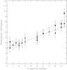 |
Fig. 1 Photospheric EW as a function of spectral subtype for luminosity class III (circle), IV (triangle) and V (square) with linear best-fit lines overplotted (solid, dotted and dashed for classes III, IV and V respectively). |
Observed standards with their corresponding stellar parameters and measured Hα equivalent widths.
A plot of the EW against spectral subtype for each luminosity class is shown in Fig. 1. The corresponding Pearson correlation coefficients for luminosity classes III, IV and V are −0.97, −0.94 and −0.88 respectively, indicating that the data are reasonably well described by a linear fit.
As an aside, the measured EWs were compared with those determined from using Kurucz models. The model was found to underestimate for earlier spectral types and overestimate for later, possibly due to the effects of line blending at the 20 Å resolution of the grid around the Hα line.
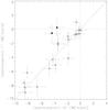 |
Fig. 2 Determined exophotospheric EWs plotted for the INT-F1 baseline. The scale has been selected to show all targets that exhibited either disk loss or formation. Targets that have been identified as losing their disk are illustrated with filled circles. The stability line (y = x) and disk loss/formation (y = 0, x = 0) axes are shown. |
4. Results and discussion
The measured EWs of the sample Hα lines are shown for each epoch in Table 1.
4.1. Complete disk loss/formation
To determine complete disk loss/formation using the calculated exophotospheric EWs, values for consecutive pairs of epochs (with corresponding baselines of INT – F1 (~10 years), F1 − F2 (~2 months), F2 – F3 (~9 months) and F3 – F4 (~3 months)) were plotted against each other; see Fig. 2 for an example plot. Candidates for disk loss were selected by identification of those targets that lay off the stability line (where no EW change could reliably be inferred), but whose EW and associated error lay within the disk loss (y = 0) axis. Likewise, candidates for disk formation were selected using similar criteria, except only those that lay within the disk formation (x = 0) axis were selected. The resulting phase-changers are shown with filled symbols in Fig. 2. As phase-changing was seen to occur only over the timescale of 10 years, only this baseline is shown.
One of the aims of this analysis was to assess if there was any correlation between spectral type and frequency of B/Be phase change. Because of the low number of targets that were identified undergoing this change, no attempt has been made to determine if a dependency on this fundamental parameter exists. Indeed, complete phase change could only be confirmed at the 3σ level for two targets in the sample, BD +05 03704 and BD +30 03227, with the longest baseline of ten years (INT – F1).
If these targets are believed to have truly changed state between B and Be phases, it is possible to estimate the approximate time over which complete phase change is expected to occur. As little observational evidence is available regarding both the distribution of phase-changing timescales and the fraction of Be stars which undergo complete phase change (most likely due to observational bias from incomplete coverage of the time domain), the following assumptions have been made:
-
the time between complete phase changes is randomly distributed (neither shorter nor longer times are preferred), and
all Be stars are subject to these episodic events of complete disk loss/formation.
With these in mind, a Monte Carlo simulation was set up to predict the number of observed phase-changers over a ten year period for different timescales (whilst constraining the minimum time to 10 years – the only baseline over which phase change was observed in this sample). The simulation was run iteratively using a 55 star dataset, recording how many were observed to change phase an odd number of times within a defined ten year window (an even number would imply that no phase change would be observed). In a sample of 55 objects, the maximum time for phase-changing to yield 2 targets observed over a ten year baseline was found to be most likely between 500 and 1000 years.
However, this maximum time comes with a possible caveat. Since Be phenomena are time variable, selection of candidate Be stars for the sample was based on heterogenous data taken from a multitide of different sources and observers that has been compiled over decades to produce a single catalogue (Jaschek & Egret 1982). If the original classification of the targets used in the sample is untrustworthy, the sample may be contaminated by B stars that have never truly shown reliable exophotospheric emission. This is certainly a real possibility for the fainter targets recorded in the catalogue, and to some extent may even be true for some of the brighter targets.
If fewer true Be targets were present in the sample, the observed fraction of phase-changers to total targets increases, increasing the frequency of phase-changes over the timescales surveyed by this study and effectively decreasing the maximum time over which the targets are expected to change phase. To determine the lower limit for the maximum time, the sample was filtered by-eye to remove targets that were always in absorption. As noted previously, due to in-filling of photospheric absorption lines this is not necessarily indicative that the star is not in emission, but serves as an upper limit to the number of stars that are non-variable, and thus could have been misclassified. The previous Monte Carlo simulation was repeated using the smaller dataset, and in this smaller sample of 44 objects, the maximum time for phase-changing to yield 2 targets observed over a ten year baseline was found to be most likely between 250 and 500 years. Finally, we note that this value will drop further if all Be stars are not subject to these episodic events of complete disk/loss formation.
4.2. Partial disk variability
In the following analysis, partial disk variability is conservatively defined as a 5σ change in EW measurement, where the previous constraints placed to force the targets to lie upon either the axis of disk loss or formation are removed. As the underlying photospheric contribution from the central star will not change between epochs, the total EW is used in the analysis of partial disk variability.
4.2.1. As a function of spectral subtype
An initial approach to the analysis of partial variability is to assess its presence over all of the possible baselines. Specifically, if an object is seen to vary in at least one of the baselines, it should be classed as variable. A plot illustrating variability over any baseline as a function of spectral subtype is shown in Fig. 3.
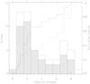 |
Fig. 3 Targets showing partial variability over any of the baselines. The hollow histogram represents the distribution of targets as a function of spectral subtype. The hatched histogram shows the distribution of those targets displaying partial variability. The cumulative fractions have been overplotted for those targets displaying partial variability (solid line) and those not (dashed line). |
Analysis regarding variability as a function of spectral subtype is presented by Hubert & Floquet (1998) who found that in a homogenously obtained Hipparcos sample of 273 Be stars, ≥98% of early Be stars (B0 – B3e) showed some degree of variability, compared with only 45% of late Be stars (B7 – B9e) over the four years during which the survey was conducted. Using the same definition of early and late types, similar figures are found in this sample, where 84% of the early Be stars in the sample were variable with only 46% of the later type showing some variation at the 5σ level over all baselines. Jones et al. (2011) find the same trend in their sample, but with only 45% of early and 29% of later types classified as variable. These smaller fractions could be the result of the statistic they use to quantify variability, which they state as being “sensitive to significant changes in disk density”.
There are several possible explanations for the observation of increased variability in earlier spectral types. It could be the case that a false-positive misclassification has introduced a bias, but such a bias would only alter the trend if later type non-variable B stars were preferentially misclassified as being variable. Filtering the sample by-eye to remove targets that were always in absorption (as in Sect. 4.1), it is found that the trend remains with 100% of the earlier type and 53% of the later type varying. Non-variability was found for 7 out of the remaining 45 stars, with all 7 stars of spectral type B5 or later.
Discounting this, the most obvious explanation would be that later spectral types are genuinely less variable than earlier. However, this may not necessarily be the complete picture, in so much that the timescales over which later types vary may not have been adequately probed by the timescales in this study.
To assess if there is any trend in the degree of variability across different timescales, pairs of epochs were grouped together to construct sets of similar baseline timescales. For the purposes of the following analysis, the baselines have been separated into <1 year (F1-F2, F3-F4), about one year (F1-F3, F2-F3, F1-F4, F2-F4) and ten years (INT-F1, INT-F2, INT-F3, INT-F4). The previous analysis was then redone using the each of the sets; the result is shown in Fig. 4. The following figures are presented for both the full dataset and the previous emission-only filtered dataset (given in brackets after the full dataset).
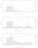 |
Fig. 4 Targets showing partial variability over <1 yr (top), ~1 yr (middle) and ~10 yrs (bottom). The hollow histograms represent the distribution of targets as a function of spectral subtype. The hatched histograms show the distribution of those targets displaying partial variability. The cumulative fractions have been overplotted for those targets displaying partial variability (solid line) and those not (dashed line). |
For partial variability over timescales less than a year, no later types could be confirmed at the 5σ level to be partially varying in either dataset, whilst 64% (79%) of the earlier type were. For timescales of around 10 years, the number of later types varying were found to be 46% in both datasets, with the number of earlier types also rising to 84% (100%). This would seem to imply some dependency of partial variability as a function of spectral type on baseline, but there is little difference in the distributions between timescales of one year and timescales of 10 years. It is worth noting that as the distribution of Be stars peaks at around a spectral type of B2 (Martayan et al. 2010) and tails off sharply towards later spectral types, quantitative statistics derived using these later objects are less certain.
A two sample Kolmogorov-Smirnov (K-S) test was also used to determine if the observed distribution of targets showing partial variability over any baseline differed from the underlying parent distribution of those which were non-variable as a function of spectral type. The calculated rejection probability for the same distribution hypothesis was found to be 75% (99%), the implication being that the stars displaying partial variability may have a different parent distribution, and thus dependency on spectral type, than those which do not.
4.2.2. As a function of rotational velocity
A plot illustrating variability over any baseline as a function of vsin i is shown in Fig. 5. From visual inspection of the plot, it would appear that stars with lower rotational velocity are less variable over the timescales probed by this study.
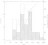 |
Fig. 5 Targets showing partial variability over any of the baselines. The hollow histogram represents the distribution of targets as a function of vsin i. The hatched histogram shows the distribution of those targets displaying partial variability. The cumulative fractions have been overplotted for those targets displaying partial variability (solid line) and those not (dashed line). |
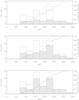 |
Fig. 6 Targets showing partial variability over <1 yr (top), ~1 yr (middle) and ~10 yrs (bottom). The hollow histograms represent the distribution of targets as a function of vsin i. The hatched histograms show the distribution of those targets displaying partial variability. The cumulative fractions have been overplotted for those targets displaying partial variability (solid line) and those not (dashed line). |
For completeness, the trend of variability as a function of vsin i is also presented using the same epoch pairings discussed in Sect. 4.2.1; the result is shown in Fig. 6. Partial variability is seen to occur for nearly 100% of those targets with the highest vsin i over all baselines, with a trend of increasing variability for longer baselines seen for stars with lower vsin i.
The two sample K-S test was also used to determine if the observed distribution of targets showing partial variability over any baseline differed from the underlying parent distribution of those which were non-variable as a function of vsin i. The calculated rejection probability for the same distribution hypothesis was found to be >99% (89%), the implication being that the stars displaying partial variability may have a different parent distribution, and thus dependency on vsin i, than those which do not.
It is noted that analysis using vsin i may be misleading. To compare stars using this quantity is to compare stars which may have different inclination angles (the angle between the rotation axis and the line of sight), spectral types and luminosity classes. A more useful parameter is the ratio of the observed rotational velocity to the critical, or break-up, velocity of the star (which in itself is a function of spectral type and luminosity class) given by ω = vrot/vcrit. However, a model-independent determination of vcrit is not attainable, and as such we do not attempt to perform analysis using this quantity.
5. Conclusions
-
The observed frequency at which transitions between the B and Be states occur is too low (2/55) for the purposes of ascertaining any dependency on spectral type or vsin i. Given this, we predict that the typical timescale between which these complete phase transitions occur is likely to be of the order of centuries.
-
Using a measure of spectral type dependency akin to that used by previous authors, we find evidence to suggest that stars of an earlier subtype may be more variable. We also find a rise in variability for later types (B7-9) when observed over baselines greater than a year. However, the weight with which this conclusion is made is limited by the small number of stars observed at later subtypes.
-
Similar to the previous conclusion, we find that stars with larger values of vsin i may be more variable. Again we note a rise in variability for stars with lower values when observed over baselines greater than a year.
-
The distributions of variable and non-variable stars with respect to both spectral type and vsin i are found to be different under a two sample K-S test.
Online material
Sample targets with their corresponding stellar parameters taken from S99.
Acknowledgments
The Liverpool Telescope is operated on the island of La Palma by Liverpool John Moores University in the Spanish Observatorio del Roque de los Muchachos of the Instituto de Astrofísica de Canarias with financial support from the UK Science and Technology Facilities Council. R.M.B. acknowledges STFC for a postgraduate studentship during which this work was undertaken. We thank the anonymous referee whose detailed review has helped to improve this paper.
References
- Banerjee, D. P. K., Rawat, S. D., & Janardhan, P. 2000, A&AS, 147, 229 [NASA ADS] [CrossRef] [EDP Sciences] [Google Scholar]
- Barnsley, R. M., Smith, R. J., & Steele, I. A. 2012, Astron. Nachr., 333, 101 [NASA ADS] [CrossRef] [Google Scholar]
- Clark, J. S., & Steele, I. A. 2000, A&AS, 141, 65 [NASA ADS] [CrossRef] [EDP Sciences] [Google Scholar]
- Collins, II, G. W. 1987, in Physics of Be Stars, eds. A. Slettebak, & T. P. Snow, IAU Colloq., 92, 3 [Google Scholar]
- Conti, P. S., & Leep, E. M. 1974, ApJ, 193, 113 [NASA ADS] [CrossRef] [Google Scholar]
- Frémat, Y., Zorec, J., Hubert, A.-M., & Floquet, M. 2005, A&A, 440, 305 [NASA ADS] [CrossRef] [EDP Sciences] [Google Scholar]
- Grundstrom, E. D., & Gies, D. R. 2006, ApJ, 651, L53 [NASA ADS] [CrossRef] [Google Scholar]
- Howells, L., Steele, I. A., Porter, J. M., & Etherton, J. 2001, A&A, 369, 99 [NASA ADS] [CrossRef] [EDP Sciences] [Google Scholar]
- Hubert, A. M., & Floquet, M. 1998, A&A, 335, 565 [NASA ADS] [Google Scholar]
- Jaschek, M., & Egret, D. 1982, in Be Stars, eds. M. Jaschek, & H.-G. Groth, IAU Symp., 98, 261 [Google Scholar]
- Jones, C. E., Tycner, C., & Smith, A. D. 2011, AJ, 141, 150 [NASA ADS] [CrossRef] [Google Scholar]
- Kogure, T. 1990, Ap&SS, 163, 7 [Google Scholar]
- Kurucz, R. L. 1979, ApJS, 40, 1 [NASA ADS] [CrossRef] [Google Scholar]
- Martayan, C., Baade, D., & Fabregat, J. 2010, A&A, 509, A11 [NASA ADS] [CrossRef] [EDP Sciences] [Google Scholar]
- Martayan, C., Rivinius, T., Baade, D., Hubert, A.-M., & Zorec, J. 2011, in IAU Symp. 272, eds. C. Neiner, G. Wade, G. Meynet, & G. Peters, 242 [Google Scholar]
- Miroshnichenko, A. S., Bjorkman, K. S., & Krugov, V. D. 2002, PASP, 114, 1226 [NASA ADS] [CrossRef] [Google Scholar]
- Morales-Rueda, L., Carter, D., Steele, I. A., Charles, P. A., & Worswick, S. 2004, Astron. Nachr., 325, 215 [NASA ADS] [CrossRef] [Google Scholar]
- Morgan, W. W., & Keenan, P. C. 1973, ARA&A, 11, 29 [NASA ADS] [CrossRef] [Google Scholar]
- Negueruela, I., Steele, I. A., & Bernabeu, G. 2004, Astron. Nachr., 325, 749 [Google Scholar]
- Percy, J. R., Hosick, J., Kincaide, H., & Pang, C. 2002, PASP, 114, 551 [NASA ADS] [CrossRef] [Google Scholar]
- Porter, J. M., & Rivinius, T. 2003, PASP, 115, 1153 [NASA ADS] [CrossRef] [Google Scholar]
- Rauw, G., Naźe, Y., Marique, P. X., et al. 2007, Information Bulletin on Variable Stars, 5773, 1 [Google Scholar]
- Slettebak, A., Collins, II, G. W., Parkinson, T. D., Boyce, P. B., & White, N. M. 1975, ApJS, 29, 137 [NASA ADS] [CrossRef] [Google Scholar]
- Steele, I. A., & Clark, J. S. 2001, A&A, 371, 643 [NASA ADS] [CrossRef] [EDP Sciences] [Google Scholar]
- Steele, I. A., Negueruela, I., & Clark, J. S. 1999, A&AS, 137, 147 [NASA ADS] [CrossRef] [EDP Sciences] [Google Scholar]
- Steele, I. A., Smith, R. J., Rees, P. C., et al. 2004, in SPIE Conf. Ser. 5489, ed. J. M. Oschmann Jr., 679 [Google Scholar]
- Townsend, R. H. D., Owocki, S. P., & Howarth, I. D. 2004, MNRAS, 350, 189 [Google Scholar]
All Tables
Observed standards with their corresponding stellar parameters and measured Hα equivalent widths.
All Figures
|
Fig. 1 Photospheric EW as a function of spectral subtype for luminosity class III (circle), IV (triangle) and V (square) with linear best-fit lines overplotted (solid, dotted and dashed for classes III, IV and V respectively). |
| In the text | |
|
Fig. 2 Determined exophotospheric EWs plotted for the INT-F1 baseline. The scale has been selected to show all targets that exhibited either disk loss or formation. Targets that have been identified as losing their disk are illustrated with filled circles. The stability line (y = x) and disk loss/formation (y = 0, x = 0) axes are shown. |
| In the text | |
|
Fig. 3 Targets showing partial variability over any of the baselines. The hollow histogram represents the distribution of targets as a function of spectral subtype. The hatched histogram shows the distribution of those targets displaying partial variability. The cumulative fractions have been overplotted for those targets displaying partial variability (solid line) and those not (dashed line). |
| In the text | |
|
Fig. 4 Targets showing partial variability over <1 yr (top), ~1 yr (middle) and ~10 yrs (bottom). The hollow histograms represent the distribution of targets as a function of spectral subtype. The hatched histograms show the distribution of those targets displaying partial variability. The cumulative fractions have been overplotted for those targets displaying partial variability (solid line) and those not (dashed line). |
| In the text | |
|
Fig. 5 Targets showing partial variability over any of the baselines. The hollow histogram represents the distribution of targets as a function of vsin i. The hatched histogram shows the distribution of those targets displaying partial variability. The cumulative fractions have been overplotted for those targets displaying partial variability (solid line) and those not (dashed line). |
| In the text | |
|
Fig. 6 Targets showing partial variability over <1 yr (top), ~1 yr (middle) and ~10 yrs (bottom). The hollow histograms represent the distribution of targets as a function of vsin i. The hatched histograms show the distribution of those targets displaying partial variability. The cumulative fractions have been overplotted for those targets displaying partial variability (solid line) and those not (dashed line). |
| In the text | |
Current usage metrics show cumulative count of Article Views (full-text article views including HTML views, PDF and ePub downloads, according to the available data) and Abstracts Views on Vision4Press platform.
Data correspond to usage on the plateform after 2015. The current usage metrics is available 48-96 hours after online publication and is updated daily on week days.
Initial download of the metrics may take a while.