| Issue |
A&A
Volume 556, August 2013
|
|
|---|---|---|
| Article Number | A121 | |
| Number of page(s) | 11 | |
| Section | Numerical methods and codes | |
| DOI | https://doi.org/10.1051/0004-6361/201219918 | |
| Published online | 07 August 2013 | |
Identification of metal-poor stars using the artificial neural network
1
Indian Institute of Astrophysics, Koramangala, 560034
Bangalore, India
e-mail: giridhar@iiap.res.in; aruna@iiap.res.in
2
Cerro Tololo Inter-American Observatory,
NOAO, Casilla 603, La Serena, Chile
e-mail: akunder@ctio.noao.edu
3
CREST Campus, Indian Institute of Astrophysics,
562114
Hosakote,
India
e-mail: muneers@iiap.res.in
4
Vainu Bappu Observatory, Indian Institute of
Astrophysics, 635701
Kavalur,
India
e-mail: selva@iiap.res.in
Received: 29 June 2012
Accepted: 23 May 2013
Context. Identification of metal-poor stars among field stars is extremely useful for studying the structure and evolution of the Galaxy and of external galaxies.
Aims. We search for metal-poor stars using the artificial neural network (ANN) and extend its usage to determine absolute magnitudes.
Methods. We have constructed a library of 167 medium-resolution stellar spectra (R ~ 1200) covering the stellar temperature range of 4200 to 8000 K, log g range of 0.5 to 5.0, and [Fe/H] range of −3.0 to +0.3 dex. This empirical spectral library was used to train ANNs, yielding an accuracy of 0.3 dex in [Fe/H] , 200 K in temperature, and 0.3 dex in log g. We found that the independent calibrations of near-solar metallicity stars and metal-poor stars decreases the errors in Teff and log g by nearly a factor of two.
Results. We calculated Teff, log g, and [Fe/H] on a consistent scale for a large number of field stars and candidate metal-poor stars. We extended the application of this method to the calibration of absolute magnitudes using nearby stars with well-estimated parallaxes. A better calibration accuracy for MV could be obtained by training separate ANNs for cool, warm, and metal-poor stars. The current accuracy of MV calibration is ±0.3 mag.
Conclusions. A list of newly identified metal-poor stars is presented. The MV calibration procedure developed here is reddening-independent and hence may serve as a powerful tool in studying galactic structure.
Key words: stars: solar-type / stars: fundamental parameters
© ESO, 2013
1. Introduction
Metallicity estimates for large samples of stars among different Galactic components can provide a wealth of information on the structure and formation of our Galaxy. Extremely metal-poor stars are the relics of early Galaxy, while moderately metal-poor stars can provide indications of whether it is a thick or thin disk when supplemented by additional information such as the kinematics of these objects. A high spectral resolution follow-up of these metal-poor stars (identified mostly through low- and intermediate-resolution spectral surveys) has resulted in identifications of exotic objects such as very metal-poor (VMP), extremely metal-poor (EMP), ultra metal-poor (UMP), and hyper metal-poor (HMP; explained in Beers & Christlieb 2005), which show different degrees of metal deficiencies. Among these metal-poor class, subclasses comprising carbon-enhanced metal-poor stars (CEMPs) have also been identified, which show a wide range in s- and r-process element enhancements. These objects are important tools for understanding the enrichment of the interstellar medium (ISM) caused by stars of different mass range in our Galaxy.
Intrinsic luminosity is another important parameter that not only helps in deriving the distances of the objects, but also helps in distinguishing objects at different evolutionary stages. The photometric determination of MV, however, requires a good reddening estimate. The spectroscopic approaches based on line strengths, line ratio, and profiles of H i, Ca ii, etc. are reddening independent. A list of luminosity-sensitive features for different spectral types can be found in Gray & Corbally (2009), and a condensed review in Giridhar (2010).
A large number of metal-poor stars have been identified with the help of earlier surveys such as the HK Survey (Beers et al. 1992). However, multi-object spectrometers like 6df on the UK Schmidt telescope (Watson et al. 1998), AAOMEGA at the Anglo-Australian Telescope (AAT) (Sharp et al. 2006), and the LAMOST project (Zhao et al. 2006) can provide a large number of spectra per night. The ongoing and future surveys and space missions will collect a vast amount of spectra for stars belonging to different components of our Galaxy and nearby galaxies. The wide variety of objects covered in these surveys require good pipelines for data handling and automated procedures that are efficient as well as robust in deriving accurate stellar parameters that are essential ingredients in studying the structure and evolution of our Galaxy.
Several automated methods of spectral classification and parametrization such as the minimum distance method (MDM), the gaussian probabilistic model (GPM), the principal component analysis (PCA), and the neural network have been developed over the last two decades. These methods have been summarized in Bailer-Jones (2002).
These automated methods differ in two major ways. Real stellar spectra of well-known calibrated stars, referred to as the empirical library, are employed by some groups (including us), while others prefer using a synthetic spectral library. Both approaches have their merits and disadvantages. Synthetic spectra depend on the quality with which the model atmosphere (often assuming local thermodynamic equilibrium) represents actual stars, and the line lists used are sometimes poor; in particular the line data for molecular lines are not very accurate. Our attempt at validating these line lists by comparing the synthetic spectra with spectra of well-known stars has shown disagreements that indicate that there are unidentified lines or that the oscillator strengths of poor quality. The problem is more severe for cool stars with molecular lines.
In empirical libraries, the stars are assigned a spectral class based upon the appearance of spectral features and therefore are model independent. Earlier reference libraries did not have the required uniform range in atmospheric parameters. The empirical libraries assembled by Jacoby et al. (1984), Pickles (1985), and Silva & Cornell (1992) mostly contained solar-metallicity objects; the last two libraries also have lower resolution. The libraries assembled by Worthey et al. (1994) and Kirkpatrick et al. (1991) had lower resolution, and the library by Serote Roos et al. (1996) had insufficient spectral coverage. At the inception of our program (more than a decade ago) the database of stellar libraries was not satisfactory (particularly for metallicity coverage), hence we chose to develop our own reference library. The situation has changed considerably now. In the past decade, several new empirical libraries providing good spectral coverage at good resolution (R ~ 2000 or better) have been developed. For the optical region, libraries such as STELIB (Le Borgne et al. 2003), ELODIE (Prugniel & Soubiran 2004; Prugniel et al. 2007), INDO-US (Valdes et al. 2004), and more recently MILES (Sánchez-Blázquez et al. 2006) have been provided while NGSL (Gregg et al. 2006), IRTF-Spex (Rayner et al. (2009), and XSL (Chen et al. 2011) provide extended coverage from the ultraviolet to the infrared. With the help of softwares such as ULySS (Koleva et al. 2009) large samples of stars can be classified and parametrized (see e.g. Prugniel et al. 2011). These empirical libraries are very important tools for building population-synthesis models and also for the automated classification and parametrization of stars. Notwithstanding its modest size, the reference library developed by us is very useful for the present problem because of its uniform coverage in metallicity, temperature, and gravity.
From the medium-resolution spectra metal-poor stars have been detected using different approaches; some are based upon the usage of strong features such as the Ca II lines (e.g. Allende Prieto et al. 2000 on INT spectra), while others employ PCA or even full spectra (e.g. Snider et al. 2001). A good account of stellar parametrization approaches developed for handling data from different surveys can be found in the volume edited by Bailer-Jones (2008).
In this paper we used the artificial neural network (ANN) to estimate stellar parameters Teff, log g, and [Fe/H] and MV for a modest sample of candidate metal-poor stars using medium-resolution spectra.
List of observed stars and their parameters.
In Sect. 2 we describe the stellar spectra database developed by us and the subset used for calibrating the ANN. Section 3 describes the observations and spectral analysis. Section 4 deals with the network configuration and the adopted network-training approach. We present in Sect. 5 the atmospheric parameters and calibration errors and the use of trained networks to estimate the parameters for a sample of candidate metal-poor stars and some unexplored field stars. The determination of absolute magnitudes is presented in Sect. 6, derived parameters for candidate metal-poor stars are given in Sect. 7. We summarize our results in Sect. 8.
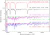 |
Fig. 1 Spectra of a selected sample of stars with near-solar metallicity displayed in decreasing temperature sequence from top to bottom. The spectra of a few metal-poor stars are superposed on solar-metallicity stars of similar temperatures. The atmospheric parameters Teff, log g, and [Fe/H] for each star are given in parenthesis. |
2. Calibrated stars
We have initiated a program for the definite identification of metal-poor candidates from different surveys such as the objective prism survey of Beers et al. (1992), which is generally referred to as the HK survey, the Edinburgh − Cape blue-object survey by Stobie et al. (1997), and the high tangential velocity objects listed by Lee (1984). During 1999–2001 we obtained spectra of a modest sample and also a good number of stars of known parameters. The semi-empirical approach adopted in Giridhar & Goswami (2002) resulted in identifying and parametrizing the metal-poor star candidates at a very slow pace, hence we chose to explore an ANN-based approach. Our earlier attempt at using the spectra of calibrated stars from the known empirical library (e.g. Jacoby et al. 1984) for training the network and then employing them for parametrizing our sample proved to be difficult despite our attempts at matching the resolution of two spectra. We faced convergence problems, and the calibration errors were unacceptably large. The spectral libraries available then also had no stars with good coverage in metallicity.
On the other hand, using stellar spectra of calibrated stars obtained with the same instrument configuration and comprising stars evenly distributed in parameter space yielded a very good calibration accuracy even for calibrated samples of modest size. It should be noted that the spectral resolution and spectral coverage of our spectra are well suited for our objective.
We therefore created a library of observed stellar spectra for stars with well-determined parameters (adding more spectra in 2004–06), which was used for training ANNs. These were used to estimate the astrophysical parameters, Teff, log g, [Fe/H] , and MV for a modest sample of unexplored field stars using medium-resolution stellar spectra.
Our database of stars with known spectral classification and parallaxes is presented in Table 1, which contains the star name, the Hipparcos number, the V magnitude, (B − V), log g, Teff, [Fe/H] , and references for the stellar [Fe/H] . Many objects were observed more than once. These objects with known atmospheric parameters were selected primarily from Gray et al. (2001), Allende Prieto & Lambert (1999), Snider et al. (2001), and Cayrel de Strobel et al. (2001). Gray et al. (2001) have calculated atmospheric parameters with the following uncertainties: 80 K in Teff, 0.1 in log g, and 0.1 in [M/H]. The temperatures tabulated by Allende Prieto & Lambert (1999) have an uncertainty of 200 K, while the uncertainty in log g varies from ±0.1 at log g of 4.5 to as much as ±0.5 at log g of 2.2. The uncertainties in the Snider et al. (2001) data are the following: 150 K in Teff, 0.3 in log g, and 0.2 in [Fe/H] . We also made use of the [Fe/H] derived from the high-resolution spectroscopy of the individual stars available in literature and those from the Elodie data base (Soubiran et al. 1998), whose parameter uncertainties are 145 K in Teff, 0.3 in log g, and 0.2 in [Fe/H] . The 73 metallicity calibration stars with known log g, Teff, and [Fe/H] contained in Table 1 (full table available in electronic form) are indicated with an asterisk mark. We observed more than two hundred stars and rejected those with binarity or other peculiarities such as Ap-Am spectra and those with emission lines. Some spectra were rejected due to poor signal to noise ratios (S/N).
3. Observation and data handling
The spectra were obtained using a medium-resolution Cassegrain spectrograph mounted on the 2.3 m Vainu Bappu Telescope at VBO, Kavalur, India. When used with a grating of 600 grooves mm-1 and a camera of 1500 mm focal length, the spectrograph gives an average dispersion of 2.6 Å per pixel. During the extended period of several years, over 200 medium-resolution spectra were obtained. The spectral coverage is 3800–6000 Å. The spectra were recorded on a 1K × 1K CCD (with Thomson TH77883) with a pixel size of 24 μ. The setup gave a two-pixel resolution of 1200.
The reduction and analysis of the spectroscopic data were performed using the standard spectroscopic packages in IRAF. All CCD frames were bias-corrected, response-calibrated using dome-flat spectra, and cleaned for cosmic rays. Even before converting them to wavelength scale, the extracted spectra were aligned accurately using a script to ensure that a given spectral feature fell on the same pixel number in all spectra. This procedure has the disadvantage that radial velocity information is not retrieved. No absolute flux calibration was performed. For fainter stars 2−3 exposures were combined to attain an S/N of at least 50. For the continuum-fitting we adopted a procedure similar to that given in Snider et al. (2001). The spectra exhibiting emission lines were excluded from the sample. The spectra were trimmed such that all spectra (700 pixels) covered exactly the same spectral region. The alignment of the spectra is crucial to obtain the desired accuracy. Figure 1 shows representative stars from our sample; the stars with near-solar metallicity arranged in decreasing temperature sequence from top to bottom. We superposed the spectra of metal-poor stars with similar temperature and show their atmospheric parameters Teff, log g, and [Fe/H] within parenthesis.
4. Atmospheric parameters of the training set
Table 1 lists the atmospheric parameters [Fe/H] , Teff, and log g compiled from the literature and adopted for each star in our study. We took particular care to select stars that span a wide range in [Fe/H] , Teff, and log g; these values were used to train the ANNs; the reference for [Fe/H] is given in the last column of Table 1. These [Fe/H] are estimated using high-resolution spectra and model atmospheres, hence their accuracy probably is about ±0.2 dex. The stars used for metallicity correction (with known [Fe/H] , Teff, and log g) are indicated by an asterisk following the star name. We used the back-propagation ANN code developed by B.D. Ripley (see Ripley 1993, 1994). The ANN configuration is same as that employed in our earlier work (Giridhar et al. 2006). Separate ANNs were trained for each parameter.
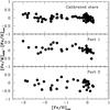 |
Fig. 2 [Fe/H]ANN − [Fe/H]Cat versus their catalog values, [Fe/H]Cat for all calibrated stars (top panel). The middle panel shows the result for part 1 obtained using weights from the ANN trained for part 2. In the bottom panel the weights from part 2 are applied to part 1. The rms error for the full sample (top panel) is 0.15 dex, for part 1 (middle panel) it is 0.31 dex, and for part 2 (bottom panel) it is 0.22 dex. |
5. ANN atmospheric parameter results
5.1. Metallicity, [Fe/H]
The top panel in Fig. 2 shows a plot of the [Fe/H] residuals obtained using the ANN for the 73 stars against their [Fe/H] taken from the literature and given in Table 1. The [Fe/H] metallicities range from −3.0 dex to 0.3 dex, and the reduced mean scatter about the line of unity is 0.15 dex. The [Fe/H] estimates quoted in the literature often have uncertainties in the range 0.2−0.4 dex. To test the goodness of the ANN, we divided the sample into two parts and trained the network separately on each part. Then the weights of ANN trained for part 1 were used to estimate [Fe/H] for the stars in part 2. The middle and bottom panels of Fig. 2 show an rms error of 0.31 and 0.22, which is indicative of the accuracy with which the ANN can predict the metallicity of a given star within the trained metallicity range.
Using the weights from the ANN trained for the sample of calibrated stars, the metallicity of the candidate metal-poor stars could be estimated. These estimates were subjected to independent tests to avoid higher temperature – low-metallicity degeneracy, but they were still useful in segregating the stars of near-solar metallicity ([Fe/H] in −0.5 to +0.3 dex range) from significantly metal-poor objects with [Fe/H] < −0.5 dex.
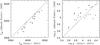 |
Fig. 3 Comparison of Teff and log g values for stars common between Allende Prieto & Lambert (1999) and Gray et al. (2001). |
5.2. Temperature and surface gravity
The literature contains a larger number of stars with good estimates of Teff and log g values compared with those with [Fe/H] values. For stars with near-solar metallicity we used temperatures and gravities given in Allende Prieto & Lambert (1999) and Gray et al. (2001) for temperature and calibration. For metal-poor stars Teff and log g were mostly taken from Snider et al. (2001). In Fig. 3 we plotted these parameters for the common stars to estimate systematic differences between the two works. We found that the Teff values obtained by Gray et al. (2001) are systematically higher by about 1.5% and for log g the systematic difference is 3% to 4%. Hence we believe that our compiled calibrating set is not affected by large systematic errors.
On the other hand, it should be noted that the metal-poor stars do not have strong features in their spectra because of their lack of metals, while hotter stars lack strong metallic features in their spectra because of ionization. To ensure that the ANN does not become confused by this, we divided the stars into solar metallicity ([Fe/H] > −0.5 dex) and metal-poor ([Fe/H] < −0.5 dex) groups.
We estimated the [Fe/H] for the sample stars in Table 1 with known Teff and log g using the ANN trained for [Fe/H] as explained in Sect. 5.1. We have spectra of 110 calibrated stars with near-solar metallicity and spectra of 33 metal-poor stars. We trained the temperature ANN separately for each metallicity group.
The solar-metallicity stars were separated into two random groups of 55, and a sanity check similar to that demonstrated in Fig. 2 was performed. The rms about the line of unity was found to be 150 K for both groups. As the temperatures found in the literature have errors that can be as high as 200 K, this is not surprising.
We trained two ANNs for log g, one ANN with stars with [Fe/H] < −0.5 dex, and the other with [Fe/H] > −0.5 dex. A procedure similar to that given for Teff was adopted. The accuracy of the log g estimate is in the range 0.3 to 0.5.
6. ANN absolute magnitude results
A large portion of the stars observed by us have parallax estimates. Combining the V-magnitudes with the Hipparcos parallaxes and absolute V-magnitudes, the MV could be calculated. Stars with a parallax error greater than 20% were excluded. Since most of the sample stars are nearby bright stars, the effect of interstellar reddening in most cases will be weak or even negligible. We therefore excluded this correction from our MV calculations. Our spectral region contains many luminosity-sensitive features such as wings of hydrogen lines, lines of Fe ii, Ti ii, Mg i lines at 5172−83 Å, and for later spectral types G-band blends of MgH, TiO, VO, etc. However, the same features cannot serve the whole range of spectral types; hence, we divided the sample stars into two groups based upon their temperatures. Group I had stars in the temperature range 4300−6300 K labeled Vc and group II those in the 6600−8000 K range labeled Vh. Yet another group, group III, which contains metal-poor stars Vm, was handled separately. The stars in this group have temperatures in a range similar to that of group I.
Figure 4 illustrates the errors associated with these three groups. The ANN trained for group I (with 76 stars labeled Vc in Fig. 4) could predict MV with an accuracy of 0.22 mag, while the ANN for group II (with 39 stars) attained an accuracy of 0.18. The group III of metal-poor stars had a very few stars (14) and could predict MV with an accuracy of only 0.29. An error of 0.3 mag in luminosity would result in an error of 150 parsec in distance at a distance of 1 kpc. One likely reason for MV error could be that luminosity sensitive features like lines of the Fe ii, Ti ii, and Mg i lines at 5172−83 Å are also metallicity dependent. Furthermore, the number of metal-poor stars with good parallaxes is woefully small. The large systematic error for low-luminosity objects with MV of 5 deserves to be analysed with additional data. Another possible solution is the usage of line ratios appropriate for metal-poor stars, as suggested by Corbally (1987) and Gray (1989).
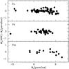 |
Fig. 4 MV ANN − MV Par versus Mv (parallax). The subset of cool stars (Vc) is plotted in the top; the middle panel contains the results for hot stars (Vh), and the bottom panel the results for metal-poor stars (Vm). |
7. Stellar parameters for the candidate metal-poor stars
The metallicity distribution of the calibrated sample is presented in the top panel of Fig. 5. The figure shows the distribution of the stars with [Fe/H] taken from the literature with a thick continuous line. An additional 110 stars with well-determined Teff and log g were lacking good [Fe/H] estimates. We determined [Fe/H] for these objects using the ANN, and their metallicity distribution is presented with a dotted line. The distribution shows that we had a good coverage of training stars in different metallicity bins.
We observed candidate metal-poor stars from the objective prism surveys of Beers et al. (1992) (BPS), the Edinburgh − Cape blue-object survey (EC) by Stobie et al. (1997), and the high tangential velocity objects listed by Lee-Sang (1984). We also included some unexplored high proper motion field stars. Using three separate ANNs, we estimated atmospheric parameters for the candidate metal-poor stars. At first, the metallicity was estimated using an ANN trained for metallicity. This helped us in separating the metal-poor stars from those of near-solar metallicity or moderately metal-poor objects. A separate ANN trained for these two groups was employed to estimate the Teff and log g for these stars. The estimated atmospheric parameters are presented in Table 2. A few stars had more than one spectrum and the small differences between the parameters estimated from each spectrum are indicative of internal errors. The (B − V) colors were available in SIMBAD for many of them, which were used to verify the temperatures estimated by the ANN. We used the calibration tables of Schmidt-Kaler (1982) to estimate the photometric temperatures. We tabulated the difference between Teff(ANN) and Teff(photometric) in Table 2. We obtained surprisingly high residuals for EC 11175-3214, EC 11260-2413, EC 13506-1845, and G 149-34. While the observed spectrum strongly supports the Teff estimated from the ANN, a misidentification cannot be ruled out. Excluding these exceptions, residuals indicate an rms error of 265 K. Many metal-poor candidate stars were near the faint limit, hence the S/N was in the range of 40–50, while most of the calibrated star spectra had an S/N higher than 100.
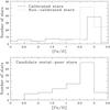 |
Fig. 5 Metallicity distribution for the calibrated sample and candidate metal-poor stars. |
Within our modest sample of stars, a good fraction (about 20%) are significantly metal-poor with [Fe/H] in −1.0 to − 2.5 range. We find that 33% of the BPS stars and 21% of the EC stars belong to the [Fe/H] range of −1.0 to −2.5. A few high proper motion Giclas objects studied also contain metal-poor stars, but the number studied is currently very small, therefore we do not offer statistics.
The bottom panel of Fig. 5 shows the metallicity distribution of candidate metal-poor stars, which shows that our candidate sample has a large portion of moderately metal-poor stars, but the fraction of significantly metal-poor star is also encouraging.
We have plotted in Fig. 6, a newly identified metal-poor star, BS 16474-0054 along with a near-solar-metalicity star of similar temperature to substantiate our findings.
With these encouraging results (notwithstanding the small sample) we propose to extend this work to a much larger sample of candidate metal-poor stars from surveys such as the HK II decribed in Beers & Christlieb (2005).
Estimated atmospheric parameters for candidate metal-poor stars.
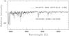 |
Fig. 6 Spectra of metal-poor stars compared with stars of similar temperature, gravity, and near-solar composition. The solid line indicates the metal-poor stars and the dashed line indicates solar-metallicity stars. The atmospheric parameters Teff, log g, and [Fe/H] for each star are given in parenthesis. |
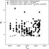 |
Fig. 7 Mv as a function of Teff for the luminosity-calibration stars and candidate metal-poor stars. |
With the help of the estimated Teff and MV, we are able to place the program stars in the H-R diagram, as shown in Fig. 7. The luminosity-calibration stars with MV taken from the literature are shown by open circles; their MV estimated from the ANN is shown by a filled circle. The difference between the two is indicative of internal errors. In both cases the Teff is the catalog value. It should be noted that our calibrated stars do not represent the local neighborhood alone since the objects were taken from different sources to encompass the required range of stellar parameters (metallicity in particular). Hence the Teff and MV diagram has a large scatter even for the calibrated stars.
A good fraction of candidate metal-poor stars are dwarfs or subgiants (which possibly are slowly evolving low-mass stars) although the calibrated stars in Table 1 also contain several giants among the significantly metal-poor stars.
7.1. Limitation of our approach and future strategy
We are aware of the problems caused by degeneracies in certain parameter domains. We avoided these sources of inaccuracies by incorporating a branching procedure that resulted in the segregation of data into meaningful subgroups. This additional step considerably improved the accuracies of the derived parameters compared with our earlier work (Giridhar et al. 2006).
It should be noted that our ANN-based approach does not allow for extrapolation. For example, the [Fe/H] network is trained for a [Fe/H] range of −3.0 to +0.3 and therefore may not give reliable results for super-metal-rich stars or Ap-Am stars. This approach is also not applicable for double-line spectroscopic binaries.
As mentioned earlier, the ANN procedure adopted here is not suitable for handling peculiar stars; however, it does provide a good estimate of Teff, log g, and metallicty for candidate metal-poor stars from the surveys mentioned previously. The Teff estimated here agree with those estimated from (B − V) within ±265 K for candidate stars with the exception of a few stars.
Although this maiden effort of estimating MV from spectral features is quite accurate for solar metallicity objects, the errors are large particularly in the low-luminosity regime for the metal-poor stars. In addition to full spectra, we propose to input some important line ratios and explore near-IR features in our future work.
8. Summary and conclusions
We have developed an empirical library of stellar spectra for stars covering a temperature range of 4200 <Teff< 8000 K, a gravity range 0.5 < log g< 5.0, and a metallicity range of −3.0 < [Fe/H] < +0.3. With the good spectral coverage of 3800–6000 Å, several spectral features showing strong sensitivity to the stellar parameters were available, which were used by the ANN in the learning process.
The procedure of pre-classifying the data and training separate ANN for each subgroup resulted in a significant increase in accuracies. Now temperatures could be estimated within ±150 K. Similarly, using of three separate ANNs for hot, cool, and metal-poor stars yielded a very good accuracy in MV calibration.
We used these trained networks primarily to detect metal-poor objects from a modest sample of unexplored objects. However, the empirical library developed may be useful for other applications and can be accessed by interested users on request. We believe that it will be useful in studying stellar population in large samples of galactic stars.
We extended the application of ANN to MV with an accuracy of ±0.3 dex. The primary application of MV is in distance determination, and the spectroscopic approach based upon the strength and profiles of the lines is independent of reddening. In addition, the MV calibration can be used for the quick identification of objects of various luminosity types in large databases containing heterogeneous objects.
Future prospects
With the ANN procedure giving the desired accuracy established here, we would like to explore a much larger sample of candidate metal-poor stars. We also need to extend the empirical library toward hotter temperatures and also overcome the poor coverage of low-gravity objects. We also contemplate including near-IR O i feature, Ca ii lines, and line ratios suggested by Corbally (1987) and Gray (1989) for the luminosity calibration of metal-poor stars. In this preliminary work, we used (for calibration) MV for nearby stars estimated from the parallaxes omitting reddening corrections. Better and enlarged samples of MV from upcoming surveys or data releases of the ongoing survey could be used to attain consistent MV accuracy in the full temperature range, which will help in understanding the evolutionary status of the candidate stars.
We have an ambitious project of observing an extended sample of F-G stars covering a broad range in galactocentric distance to study the metallicity gradient, which is known to exhibit two slopes and also some wriggles near the spiral arm locations. We hope to attain the required accuracy in metallicity by carefully binning the data in a more narrow range in temperatures and gravities, and also including important line ratios.
Acknowledgments
Sunetra Giridhar wishes to thank T. Van Hippel for his help with the ANN code. This work was partially funded by the National Science Foundations Office of International Science and Education, Grant Number 0554111: International Research Experience for Students, and managed by the National Solar Observatorys Global Oscillation Network Group. This work made use of the SIMBAD astronomical database, operated at CDS, Strasbourg, France, and the NASA ADS, USA. We thank the anonymous referees for their constructive comments, which helped us to improve the manuscript.
References
- Adelman, S. J., & Philip, A. G. D. 1994, MNRAS, 269, 579 [NASA ADS] [Google Scholar]
- Allen de Prieto, C., & Lambert, D. L. 1999, A&A, 352, 555 [NASA ADS] [Google Scholar]
- Allende Prieto, C., Rebolo, R., García López, R. J., et al. 2000, AJ, 120, 1516 [NASA ADS] [CrossRef] [Google Scholar]
- Axer, M., Fuhrmann, K., & Gehren, T. 1994, A&A, 291, 895 [NASA ADS] [Google Scholar]
- Bailer-Jones, C. A. L. 2002, Automated Data Analysis in Astronomy, 83 [Google Scholar]
- Bailer-Jones, C. A. L. 2008, in, Classification and Discovery in Large Astronomical Surveys, AIPC Conf. Proc., 1082 [Google Scholar]
- Balachandran, S. 1990, ApJ, 354, 310 [NASA ADS] [CrossRef] [Google Scholar]
- Beers, T. C., & Christlieb, N. 2005, ARA&A, 43, 531 [NASA ADS] [CrossRef] [Google Scholar]
- Beers, T. C., Preston, G. W., & Shectman, S. A. 1992, AJ, 103, 1987 [NASA ADS] [CrossRef] [Google Scholar]
- Burkhart, C., & Coupry, M. F. 1989, A&A, 220, 197 [NASA ADS] [Google Scholar]
- Cayrel de Strobel, G., Soubiran, C., & Ralite, N. 2001, A&A, 373, 159 [NASA ADS] [CrossRef] [EDP Sciences] [Google Scholar]
- Chen, Y., Trager, S., Peletier, R., & Lancon, A. 2011, JPhCS, 328, 012023 [NASA ADS] [Google Scholar]
- Corbally, C. J. 1987, AJ, 94, 161 [NASA ADS] [CrossRef] [Google Scholar]
- Edvardsson, B., Andersen, J., Gustafsson, B., et al. 1993, A&A, 275, 101 [NASA ADS] [Google Scholar]
- Giridhar, S. 2010, BASI, 38, 1 [NASA ADS] [Google Scholar]
- Giridhar, S., & Goswami, A. 2002, BASI, 30, 501 [NASA ADS] [Google Scholar]
- Giridhar, S., Muneer, S., & Goswami, A. 2006, MmSAI, 77, 1130 [Google Scholar]
- Gratton, R. G., & Ortolani, S. 1986, A&A, 169, 201 [NASA ADS] [Google Scholar]
- Gray, R. O. 1989, AJ, 98, 1049 [NASA ADS] [CrossRef] [Google Scholar]
- Gray, R. O., & Corbally, J. 2009, in Stellar Spectral Classification. Princeton Series in Astrophysics (Princeton and Oxford: Princeton Univ. Press) [Google Scholar]
- Gray, R. O., Graham, P. W., & Hoyt, S. R. 2001, AJ, 121, 2159 [NASA ADS] [CrossRef] [Google Scholar]
- Gregg, M. D., et al. 2006, in The 2005 HST calibration workshop, Vol NASA/CP2006- 214134, (Greenbelt MD: NASA), eds. A. M. Koekemoer, P., Goudfrooij, & L. L. Dressel [Google Scholar]
- Jacoby, G. H., Hunter, D. A., & Christian, C. A. 1984, ApJS, 56, 257 [NASA ADS] [CrossRef] [Google Scholar]
- Kirkpatrick, J. D., Henry, T. J., & McCarthy, D. W., Jr. 1991, ApJS, 77, 417 [NASA ADS] [CrossRef] [Google Scholar]
- Koleva, M., Prugniel, P., Bouchard, A., & Wu, Y. 2009, A&A, 501, 1269 [NASA ADS] [CrossRef] [EDP Sciences] [Google Scholar]
- Le Borgne, J. F., Bruzual, G., Pello, R., et al. 2003, A&A, 402, 433 [NASA ADS] [CrossRef] [EDP Sciences] [Google Scholar]
- Lee, S.-G. 1984, AJ, 89, 702 [NASA ADS] [CrossRef] [Google Scholar]
- Luck, R. E., & Lambert, D. L. 1981, ApJ, 245, 1018 [NASA ADS] [CrossRef] [Google Scholar]
- Luck, R. E., & Lambert, D. L. 1985, ApJ, 298, 782 [NASA ADS] [CrossRef] [Google Scholar]
- Moultaka, J., Ilovaisky, S. A., Prugniel, P., & Soubiran, C. 2004, PASP, 116, 693 [NASA ADS] [CrossRef] [Google Scholar]
- Oinas, V. 1974, ApJS, 27, 405 [NASA ADS] [CrossRef] [Google Scholar]
- Patchett, B. E., McCall, A., & Stickland, D. J. 1973, MNRAS, 164, 329 [NASA ADS] [Google Scholar]
- Pickles, A. J. 1985, ApJS, 59, 33 [NASA ADS] [CrossRef] [Google Scholar]
- Prugniel, P., & Soubiran, C. 2004 [arXiv:astro-ph/0409214] [Google Scholar]
- Prugniel, P., Soubiran, C., Koleva, M., & Le Borgne, D. 2007 [arXiv:astro-ph/0703658] [Google Scholar]
- Prugniel, P., Vauglin, I., & Koleva, M. 2011, A&A, 531, A165 [NASA ADS] [CrossRef] [EDP Sciences] [Google Scholar]
- Rayner, J. T., Cushing, M. C., & Vacca, W. D. 2009, ApJS, 185, 289 [NASA ADS] [CrossRef] [Google Scholar]
- Ripley, B. D. 1993, in Networks and Chaos: Statistical and Probabilistic Aspects, eds. O. E. Barndorff-Nielsen, J. L. Jensen, & W. S. Kendall (London: Chapman & Hall), 40 [Google Scholar]
- Ripley, B. D. 1994, in Statistics and Images, Advances in Applied Statistics, ed. K. V. Mardia (Abingdon: Carfax), 37 [Google Scholar]
- Ryan, S. G., & Lambert, D. L. 1995, AJ, 109, 2068 [NASA ADS] [CrossRef] [Google Scholar]
- Sánchez-Blázquez, P., Peltier, R. F., Jiménez-Vicente, J., et al. 2006, MNRAS, 371, 703 [NASA ADS] [CrossRef] [Google Scholar]
- Schmidt-Kaler, T. S. 1982, Landolt-Bornstein Group 6, 2b (Springer Verlag) [Google Scholar]
- Serote Roos, M., Boisson, C., & Joly, M. 1996, A&AS, 117, 93 [NASA ADS] [CrossRef] [EDP Sciences] [Google Scholar]
- Sharp, R., Saunders, W., Smith, G., et al. 2006, SPIE, 6269 [Google Scholar]
- Silva, D. R., & Cornell, M. E. 1992, ApJS, 81, 865 [NASA ADS] [CrossRef] [Google Scholar]
- Snider, S., Allen de Prieto, C., von Hippel, T., et al. 2001, ApJ, 562, 528 [NASA ADS] [CrossRef] [Google Scholar]
- Soubiran, C., Katz, D., & Cayrel, R. 1998, A&AS, 133, 221 [NASA ADS] [CrossRef] [EDP Sciences] [Google Scholar]
- Spite, M., Pasquini, L., & Spite, F. 1994, A&A, 290, 217 [NASA ADS] [Google Scholar]
- Stobie, R. S., Kilkenny, D., O’Donoghue, D., et al. 1997, MNRAS, 287, 848 [NASA ADS] [CrossRef] [Google Scholar]
- Tomkin, J., & Lambert, D. L. 1999, ApJ, 523, 234 [NASA ADS] [CrossRef] [Google Scholar]
- Tomkin, J., Lemke, M., Lambert, D. L., & Sneden, C. 1992, AJ, 104, 1568 [NASA ADS] [CrossRef] [Google Scholar]
- Valdes, F., Gupta, R., Rose, J. A., Singh, H. P., & Bell, D. J. 2004, ApJS, 152, 251 [NASA ADS] [CrossRef] [Google Scholar]
- Venn, K. A. 1995, ApJS, 99, 659 [NASA ADS] [CrossRef] [Google Scholar]
- Watson, F. G., Parker, Q. A., & Miziarski, S. 1998, Proc. SPIE, 3355, 834 [NASA ADS] [CrossRef] [Google Scholar]
- Worthey, G., Faber, S. M., Gonzalez, J. J., & Burstein, D. 1994, ApJS, 94, 687 [NASA ADS] [CrossRef] [Google Scholar]
- Zhao, G., Chen, Y.-Q., Shi, J.-R., et al. 2006, ChJAA, 6, 265 [NASA ADS] [CrossRef] [Google Scholar]
All Tables
All Figures
|
Fig. 1 Spectra of a selected sample of stars with near-solar metallicity displayed in decreasing temperature sequence from top to bottom. The spectra of a few metal-poor stars are superposed on solar-metallicity stars of similar temperatures. The atmospheric parameters Teff, log g, and [Fe/H] for each star are given in parenthesis. |
| In the text | |
|
Fig. 2 [Fe/H]ANN − [Fe/H]Cat versus their catalog values, [Fe/H]Cat for all calibrated stars (top panel). The middle panel shows the result for part 1 obtained using weights from the ANN trained for part 2. In the bottom panel the weights from part 2 are applied to part 1. The rms error for the full sample (top panel) is 0.15 dex, for part 1 (middle panel) it is 0.31 dex, and for part 2 (bottom panel) it is 0.22 dex. |
| In the text | |
|
Fig. 3 Comparison of Teff and log g values for stars common between Allende Prieto & Lambert (1999) and Gray et al. (2001). |
| In the text | |
|
Fig. 4 MV ANN − MV Par versus Mv (parallax). The subset of cool stars (Vc) is plotted in the top; the middle panel contains the results for hot stars (Vh), and the bottom panel the results for metal-poor stars (Vm). |
| In the text | |
|
Fig. 5 Metallicity distribution for the calibrated sample and candidate metal-poor stars. |
| In the text | |
|
Fig. 6 Spectra of metal-poor stars compared with stars of similar temperature, gravity, and near-solar composition. The solid line indicates the metal-poor stars and the dashed line indicates solar-metallicity stars. The atmospheric parameters Teff, log g, and [Fe/H] for each star are given in parenthesis. |
| In the text | |
|
Fig. 7 Mv as a function of Teff for the luminosity-calibration stars and candidate metal-poor stars. |
| In the text | |
Current usage metrics show cumulative count of Article Views (full-text article views including HTML views, PDF and ePub downloads, according to the available data) and Abstracts Views on Vision4Press platform.
Data correspond to usage on the plateform after 2015. The current usage metrics is available 48-96 hours after online publication and is updated daily on week days.
Initial download of the metrics may take a while.