| Issue |
A&A
Volume 556, August 2013
|
|
|---|---|---|
| Article Number | A95 | |
| Number of page(s) | 8 | |
| Section | The Sun | |
| DOI | https://doi.org/10.1051/0004-6361/201219478 | |
| Published online | 02 August 2013 | |
Flare line impact polarization
Na D2 589 nm line polarization in the 2001 June 15 flare⋆
1
Laboratoire d’Études Spatiales et d’Instrumentation en Astrophysique,
Observatoire de Paris,
5 place Jules Janssen,
92190
Meudon,
France
e-meil:
This email address is being protected from spambots. You need JavaScript enabled to view it.
2
Astronomical Institute, Academy of Sciences of the Czech Republic,
25165
Ondřejov, Czech
Republic
e-meil:
This email address is being protected from spambots. You need JavaScript enabled to view it.
Received:
25
April
2012
Accepted:
9
June
2013
Abstract
Context. The impact polarization of optical chromospheric lines in solar flares is still being debated. For this reason, additional observations and improved flare atmosphere models are needed still.
Aims. The polarization-free telescope THEMIS used in multiline 2 MulTiRaies (MTR) mode allows accurate simultaneous linear polarization measurements in various spectral lines.
Methods. In the 2001 June 15 flare, Hα, Hβ, and Mg D2 lines linear impact polarization was reported as present in THEMIS 2 MTR observations. In this paper, THEMIS data analysis was extended to the Na D2 line. Sets of I ± U and I ± Q flare Stokes S 2D-spectra were corrected from dark-current, spectral-line curvature and from transmission differences. Then, we derived the linear polarization degree P and polarization orientation angle α 2D-spectra. No change in relative positioning could be found that would reduce the Stokes parameters U and Q values. No V and I crosstalks could explain our results either.
Results. The Na D2 line is linearly polarized with a polarization degree exceeding 5% at some locations. The polarization was found to be radial at outer ribbons edges, and tangential at their inner edges. This orientation change may be due to differences in electron distribution functions on the opposite borders of flare chromospheric ribbons. Electron beams propagating along magnetic field lines, together with return currents, could explain both radial and tangential polarization. At the inner ribbon edges, intensity profile-width enlargements and blueshifts in polarization profiles are observed. This suggests chromospheric evaporation.
Key words: polarization / Sun: activity / Sun: flares / acceleration of particles
Appendix A is available in electronic form at http://www.aanda.org
© ESO, 2013
1. Introduction
According to their atomic structures, atoms and ions may generate linearly polarized line emission when collisionally excited by particles beams. Laboratory observations, made perpendicularly to a beam, show that the impact line center linear polarization degree and linear polarization direction are both particle energy dependent.
At particle energies close to threshold excitation energy, impact polarization is parallel to the beam’s travelling direction. At high energies, the polarization direction becomes perpendicular to the beam. Electrons and protons with equal velocities lead to the same polarization degree. As shown in Fig. 1 (see also Hénoux & Vogt 1998, and references therein), for a beam falling vertically on the solar chromosphere, particles with velocities close to threshold excitation velocity generate radial linear polarization. Polarization becomes tangential at higher energies.
Owing to the Na hyperfine structures, the D2 line polarization degree observed at 90deg from the particle beam direction is close to 14% at threshold energy. However, in a 200 G magnetic field or more, the polarization degree is determined by the atomic fine structure, and rises to 40% (Kleinpoppen & Neugart 1967). In solar active regions, such magnetic field intensity is expected to be present at the chromospheric level. This means a significant polarization signal is expected.
However, in the solar atmosphere additional collisional and radiative excitation processes may reduce the net polarization degree. Theoretical models and theoretical arguments for or against the generation of chromospheric line linear polarization in solar flares do exist. Štěpán et al. (2007) find that, in a flaring chromosphere represented by classical plane parallel dense and hot 2D models, radiative and collisional depolarization reduces hydrogen Hα polarization. However, filamentary flare models (Fletcher & Brown 1998) predict a low radiative and collisional depolarization level. Therefore, reliable observations are mandatory when selecting the most appropriate model.
According to various authors, Hα and Hβ lines are linearly polarized in solar flares (Hénoux & Semel 1981; Metcalf et al. 1992; 1994; Vogt & Hénoux 1996, 1999; Firstova et al. 1997, 2003, 2005; Vogt et al. 2001; Firstova & Kashapova 2002; Hénoux & Karlický 2003; Hanaoka 2003; Xu et al. 2005). On the other hand, Bianda et al. (2005), using the ZIMPOL instrument, and Hanaoka (2005) did not find any linear polarization signature in solar flares above a sensitivity level of 0.1%.
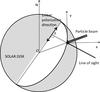 |
Fig. 1 Radial polarization orientation generated by a vertical beam of particles moving
along vertical magnetic field lines. These particles are supposed to have velocities
close to the electron Na D2 collisional excitation threshold-velocity
|

On 2001 June 15, an M6.3 flare that was following a filament eruption near 10:06 was observed from 10:07:20 to 10:30:56 UT in the NOAA Active Region 9502 by THEMIS in the MulTiRaies (MTR) multiline spectropolarimetric mode. The flare location, at S26° E41°, was favorable to impact polarization observations, and the Hα, Hβ, and Mg D2 lines (Xu et al. 2005, 2006) were found to be linearly polarized. In all cases polarization was radial or tangential, that is to say parallel or perpendicular to the flare to disk center direction. This data set contains also Na 5890.97 Å D2 line observations. The results of their analysis are reported here.
2. THEMIS flare multiwavelength polarization observations
In the MTR, multiline spectropolarimetric mode1, two I(y, λ) + S(y, λ) and I(y, λ) − S(y, λ) 2D spectra are shifted one above the other and recorded simultaneously. The Stokes parameters I(y, λ) and S(y, λ) are functions of the pixel position, y, along the spectrograph slit direction and of wavelength. These 2D spectra cover two 143 × 382 pixels bands, on a single CDD camera. Here S(y, λ) is either U(y, λ) or Q(y, λ). Each band corresponds to one arc min along the spectrograph slit direction y and 0.70 nm in the spectral direction. The spectrograph slit is parallel to the celestial north direction. Scans were made by moving the solar image perpendicularly to the slit, so in the x spatial direction (see Fig. 1). Below, the space and wavelength dependence will not be explained. In what follows, all Stokes parameters S(y, λ) will be simply written as S.
2.1. Definition of the Stokes parameters measured with THEMIS and observational mode used
The axis used to define the Stokes parameters Q, U, and I are represented in Fig. 2:
 The
U−axis is parallel to the celestial north direction, so
parallel to the slit y direction. U,Q, and
I are all functions of y and λ. For
Q ≠ 0, the angle θ between the direction of the linearly
polarized part of the radiation and the U−direction is given
by
The
U−axis is parallel to the celestial north direction, so
parallel to the slit y direction. U,Q, and
I are all functions of y and λ. For
Q ≠ 0, the angle θ between the direction of the linearly
polarized part of the radiation and the U−direction is given
by  and
for Q = 0:
and
for Q = 0:  Here
θ is counted clockwise. Then, from the Stokes parameters
I, U, Q, the polarization degree
P and the angle α between linear polarization and
flare to disk center directions were derived:
Here
θ is counted clockwise. Then, from the Stokes parameters
I, U, Q, the polarization degree
P and the angle α between linear polarization and
flare to disk center directions were derived:  , and
α = Θ−ΘAR. Here ΘAR is the
angle between the flare to disk center direction OF and the
U−axis. ΘAR is equal to 65°. Both
P and α are 2D
P(y, λ) and α(y, λ)
functions.
, and
α = Θ−ΘAR. Here ΘAR is the
angle between the flare to disk center direction OF and the
U−axis. ΘAR is equal to 65°. Both
P and α are 2D
P(y, λ) and α(y, λ)
functions.
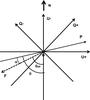 |
Fig. 2 Orientation, relative to the celestial north direction, N, of the axes used to define the Stokes parameters. OF indicates the Sun center to flare direction. ΘAR is the angle between this direction and the celestial north direction. |
2.2. THEMIS polarization measurements
On 2001 June 15, a GOES class M6 flare, 1N in the optical range, with radio and hard X-ray emissions (Fárník et al. 2001; Hénoux & Karlický 2003; Xu et al. 2005) starting at about 10:00 UT, was observed in AR 9502 (S27°E43°). The hard and soft X-ray emission time profiles are shown in Fig. 3. This flare was associated with a filament explosive rise (Brosius 2003; Romano et al. 2005). A coronal loop that was initially ascending with the filament began to contract, as soon as the filament rose (Liu & Wang 2009), and exploded.
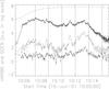 |
Fig. 3 2001 June 15 flare: GOES soft X-ray 1−8 A flux (dashed-dotted) in arbitrary units and HXRBS (Fárník et al. 2001) hard X-rays 19−29 keV (full line), 44−67 keV (dotted line) and 100−147 keV (dashed line) count rates. Vertical lines show times of observations presented in Figs. 4 and 6. |
From 10:07:20 until 11:01:49, the flaring active region AR 9502 was scanned sixteen times along the x direction. Each 90 s scan was made in 20 steps separated by 2.5 s of arc in space and 4.5 s in time. Along the spectrograph entrance slit, the spatial separation between two adjacent pixels was 0.42 arcsec. The slit width covered 1 arcsec along y on the solar surface. For a given solar image position on the spectrograph slit, two simultaneous I + S and I − S spectra were recorded successively, for S alternatively equal to U and Q. To reduce the time delay between two successive sets of U and Q measurements, there was no measurement of the V signal. A V contribution to the U or Q signals should be limited to the wavelength-shifted σ components in longitudinal magnetic fields regions, generating systematic and time-stable line wing linear polarization signals, which are not observed (see A.3).
Data were corrected from dark-current and spectral-line curvature. There was no significant size and relative position errors in the x and y directions (see Appendix). Then, as explained in Sect. 2.1, the polarization degree P and polarization orientation angle α were derived. The main false polarization source being the intensity gradient, a very accurate positionning of the I + S and I − S signals is needed. As shown in the Appendix, false polarization due to intensity crosstalk does not exceed 0.4%. Linear polarization directions are predominantly radial and tangential. D2 line linear polarization degree, below 0.4% in the wings, could exceed 4% at line center, and could even reach 8% at some locations and times.
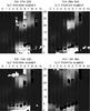 |
Fig. 4 Polarization pseudo-spectroheliograms of 2001 June 15th two-ribbon flare derived from four observing time sets. Intensity levels are in grey. y axis is labeled in arcsec. Each x axis label identifies a narrow 2D spectra in a set of eleven adjacent and successive 2D spectra of wavelength width 0.032 nm, covering 11 pixels. They correspond to scans made along the x direction (with a δx 2.5 arcsec scan step). Regions with Na D2 linear polarization degree higher than 3%, and with either tangential or radial polarization directions are in black or white. On the 10H 07M 20S pseudo-spectroheliogram, four letters, A, B, C, D, indicate locations where line intensity, polarization degree and orientation profiles were computed (see Fig. 5). |
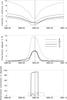 |
Fig. 5 Line intensity and line polarization degree spectral profiles (top) and line polarization orientation spectral profile (bottom), at locations A, B, C, and D (see Fig. 4). Dashed vertical lines give wavelength position of the Na D2 line, when solar rotation is taken into account. |
2.3. Pseudo-spectroheliograms of active region 9502
In every 2D spectrum, a narrow δλ wavelength band, centered on line center and covering 0.025 nm (eleven pixels along x direction), was selected. For each time sequence (for each scan), a set of eleven of such narrow spectra were selected among twenty, adjacent in space and consecutive in time. The interval δx between them is equal to the 2.5 arcsec scan step. In the y direction, 2.5 arcsec covers 6 x pixels. Therefore, to correct from this 11/6 x-scale to y-scale ratio, appropriate rescaling was used. Four of these pseudo-spectroheliograms − from 10:07:20 to 10:13:38 − are shown in Fig. 4.
The flare appears as a two-ribbon flare, both in intensity and in polarization. No significant polarization is observed in the brightest parts of the flare. As seen in Fig. 4, radial and tangential polarization higher than 4% are observed on outer (regions A, B, and D) and inner ribbons edges (region C), respectively. As the ribbons separate, Na D2 polarization fades away. At flare beginning, areas covered by radial polarization dominate the ones covered by tangential polarization. Later, tangential polarization regions become preponderant (see Figs. 4 and 6). This could be an artifact, since ribbon separation makes the outer edges leave the field of view.
2.4. Intensity and polarization line profiles on flare ribbon edges
The intensity, polarization degree, and polarization orientation profiles at locations A, B, C, and D are drawn in Fig. 5. These profiles have been selected at positions along the slit where the line core polarization is the higest. In line wings, the polarization degree is below 0.05%, while line center polarization varies from 4% to 8%. Conditions of energy transport in the 2001 June 15 flare derived from these profiles are discussed in following section.
3. Causes of the 2001 June 15 flare’s Na D2 line polarization
In laboratory plasmas, collisional excitation of Na atoms by beams of electrons or protons leads to linearly polarized Na D2 line emission. This linear polarization changes from parallel to perpendicular to the beam direction at a turnover energy of about 9 keV for protons (Balança & Dubois 2001) and 5 eV for electrons (Kleinpoppen 1969). The measured D2 line threshold polarization is parallel to the beam direction and reaches about 17% (Stumpf et al. 1978). At higher energies, polarization becomes perpendicular, with a polarization degree close to 20% for 20 keV protons and 10 eV electrons (energies at which the Na (3p, 3d) excitation cross section has a maximum) as computed by Balança & Dubois (2001).
In solar atmosphere, other excitation processes − radiative or collisional − have to be taken into account. Using a classical 2D dense and plane parallel flare model, Vogt et al. (1997) found that Hα -line impact polarization is strongly reduced by the local radiation field and by the thermal local electron contributions to line formation. Fine structure transitions induced by collisions would still reduce the polarization level. Using a more refined radiative transfer code, S˘tĕpán et al. (2007) reached a similar conclusion.
However, the flaring atmosphere is presumably filamentary. Fletcher & Brown (1998, see references therein) attributed the observed Hα-line impact polarization to fragmented evaporative upflows. They suggested that Hα polarization is generated in discrete upward chromospheric flows surrounded by a static and relatively cold atmosphere. In this model the upward flows are constituted by ionized hydrogen. The interaction between these protons and the laterally diffusing neutral hydrogen takes place at the interface between the flow and the quiet-atmosphere, with an interface of thickness of about 102 m. In such a fragmented flare atmosphere, the external radiation field is formed in the quiet surrounding atmosphere. Therefore, its contribution to line formation is significantly lower than in a hot and dense 2D classical flare atmosphere. Ignoring the radiative contribution to line formation, Fletcher and Brown applied their model to radially polarized Hα line formation. Radial polarization was found to be generated. The highest polarization compatible with observational results is obtained for filaments with a radius comparable to the interaction distance. This model could well be applied to Na D2 line polarization observations.
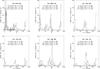 |
Fig. 6 Number dN(θ) of pseudo-spectroheliograms pixels with polarization orientation equal to θ +/− one degree, as a function of θ. Three sets of pixels, with a polarization degree respectively higher than 6, 4, and 3%, have been selected. The associated histograms are drown in full, dashed, and dotted lines. |
3.1. Conditions of energy transport in the 2001 June 15 flare as derived from impact polarization observations
Na D2 line polarization intensity, orientation, and flare energy transport mechanisms are all linked. The polarization could be due either to particle beams with return currents, to neutral beams, to chromospheric evaporation, or to heat conduction. We propose below a scenario where chromospheric evaporation and return currents in connection with electron beams could explain the main characteristics of Na D2 line linear polarization on the outer and inner ribbon edges.
On outer ribbon edges Na D2 linear polarization is nearly radial. No significant Doppler shift is observed. Low-energy protons could be responsible for such polarization. However, additional arguments do support the hypothesis of electron beams being responsible for such polarization; i.e., hard X-ray emission is observed in this flare until 10:21 UT, and it is known that hard X-ray sources are observed only on outer ribbon edges (Czaykowska et al. 1999). Return currents are presumably associated with electron beams. They have been shown as able to contribute significantly to Hα line excitation and impact polarization (Karlický & Hénoux 2002; Hénoux & Karlický 2003). They can also contribute to Na D2 line impact polarization.
Return currents are carried by electrons of density
 and
velocity
and
velocity such that
 where
Φ is the number flux of beam superthermal electrons, Φ is equal to
where
Φ is the number flux of beam superthermal electrons, Φ is equal to
 , and
, and
 and
and
 are the beam
electrons mean density and mean velocity. The return current electron number density
can be either
the background electron number density ne or the runaway
electron density. Return current electrons can also be produced in thin double layers
formed in the electron-beam-return current system (Karlický 2012). is expected
to be higher than , and
consequently the electron velocity in a return
current is believed to be lower than the electron velocity of a monoenergetic electron
beam. Then, return current electrons energies and beam electrons energies could well be
respectively below and above the turnover energy. In such a case, radial and tangential
linear polarization should be generated. The net polarization orientation will depend on
their relative contributions.
are the beam
electrons mean density and mean velocity. The return current electron number density
can be either
the background electron number density ne or the runaway
electron density. Return current electrons can also be produced in thin double layers
formed in the electron-beam-return current system (Karlický 2012). is expected
to be higher than , and
consequently the electron velocity in a return
current is believed to be lower than the electron velocity of a monoenergetic electron
beam. Then, return current electrons energies and beam electrons energies could well be
respectively below and above the turnover energy. In such a case, radial and tangential
linear polarization should be generated. The net polarization orientation will depend on
their relative contributions.
Beam and return current electron fluxes are equal. Consequently, return current and beam electrons contributions to line intensity and polarization are proportional to their excitation cross sections. Particle excitation cross sections decrease with increasing energy. Therefore, the polarization direction will be close to the one generated by the return current, hence close to radial. Such mechanism is presumably at work on the outer edges. Here, the polarization direction deviates from radial by only 10°. This slight departure from radial direction, as well as the 5° deviation from the tangential direction at location C, is presumably due to deviations from the verticality of the chromospheric magnetic lines of force. The 2D spatial distribution of the transverse photospheric magnetic field (Xu et al. 2005) shows deviations from the radial direction that agree with this hypothesis.
Tangential Na D2 linear polarization is located on inner flare ribbon edges (like at location C in Fig. 4). There, the intensity profile is wide and asymmetrical (Fig. 5), indicating the presence of turbulent motions. In addition, the associated polarization profile does show a strong blue wing, that could well be due to upward motions of Na atoms excited by impact in fragmented evaporative upflows. This observation agrees with the Fletcher & Brown (1998) model based upon evaporation in filamentary channels. Initially made to explain Hα line polarization observations, this model assumes an electron and proton upward flow speed of 500 km s-1 (electron and proton energies of 1ev and 2 keV, respectively). A two to three time higher velocity is compatible with the blueshifts observed both in the polarization and intensity line profiles. Then, the electron and proton energies in the upward flow would exceed, respectively, the 5 eV (electrons impact excitation) and 9 keV (proton impact excitation) turnover energies above which tangential polarization is generated. Therefore, fragmented evaporating upflows can explain the tangential polarization observed on inner ribbon edges.
EUV observations agree with a chromospheric evaporation model. In the 2001 June 15 flare, the flare precursor seen in O III and O V preceded the onset of the Fe XIX emisssion by nearly two minutes. This led Brosius (2003) to conclude that the first response to flare’s magnetic energy release was not in the corona but rather at the chromospheric level. At 10:05, the full OIII line profile of a 2′′ × 20′′ area above the O III-O V flare kernel is blueshifted. At 10:07, this profile becomes redshifted, even if a blueshifted component is still present. This agree with the blueshift observed at location C and with the hypothesis of tangential polarization as the signature of chromospheric evaporation. However, we cannot prove that the O III-O V flare kernel is located above the C position.
4. Conclusions
Linear impact polarization was already observed on 15 June 2001 flare in Hα, Hβ and Mg D2 lines. Analysis of Na D2 line linear polarization spectra confirms the existence of impact polarization. Negligible over flare kernels, the polarization degree reaches 3 to 9% at the ribbon edges. The highest polarization is observed at the time of the first 19−29 keV hard X-ray emission peak. Such a high degree of polarization does support a filamentary solar-flare model.
The polarization is found to be radial at outer ribbons edges, and tangential at their inner edges. This change in polarization direction should be related to differences in the conditions of energy release and energy deposit at these chromospheric edges. Filamentary chromospheric evaporation, acting presumably at location C, together with electron beams and return currents (at locations A, B, and D), are good candidates for explaining the polarization temporal and spatial characteristics.
Online material
Appendix A: Flare data processing
Some authors have reported an Hα-line impact polarization level below 1% in flares. Others like Bianda et al. (2005) did not find any clear linear polarization signature above a sensitivity level of 0.1% in Hα flare observations.Their measurements were made in filter mode with 1′′ × 1′′ pixels and 2 s integration time. Stokes polarization images were obtained by averaging over a 10′′ × 10′′ area, covered in 40 s. Polarization islands in THEMIS observations do not exceed 4′′ × 4′′; i.e., Bianda et al. integrated their measurements over a six times bigger area. For uniform intensity, after integrating over such extended area, a 6% polarization degree would go down below 1%. Moreover, including brighter flare unpolarized regions in this area − which extends over 24 pixels along the slit − would make the polarization degree go further down to the 0.1 to 0.5% level. A 40 s. integration time would reduce this level even more. Bianda et al. observations and the ones presented here were made in Na D2. The set of THEMIS mutiwavelength simultaneous observations included Hα, Hβ, and Mg lines. All these lines were also found to be polarized (Xu et al. 2005, 2006).
After rebinning, the complementary Bianda et al. spectrograph observation of a X17.1 flare has temporal and spatial resolutions (5 arcsec, 10 s) lower than the ones given by THEMIS. The arguments given above also apply to these measurements. Moreover, the spectrograph entrance slit may not have been put at the right place at the right time.
In high-frequency polarization measurements, Hanaoka (2005) find degrees of polarization in the 0.5 to 1% range. However, these measurements include contributions of all flare kernels over one minute of time. As in Bianda et al. observations, unpolarized bright flare kernel intensity may reduce the flare edge’s polarization signal by one order of magnitude.
These contradictory results justify discussing THEMIS data calibration and Intensity and Stokes V crosstalks below.
Appendix A.1: Flare data calibration
Flat-field and dark-current measurements are made before and after each set of active region observations. These flat-field measurements were used to correct the spectra from line curvature. They were also used for positioning the two spectra in y and correcting for possible y size differences.
The optical paths of the two I ± S beams, where
S could be either U or Q, are
different. Therefore, even for unpolarized light, as in line wings, observed
T = (I + S)/(I − S)
intensity ratio differs from unity. Relative correction factors
Rl and
Rr
(R = 1/T) have to be applied to
band 0 (I + S) left and right line wings
(wavelengths λl and
λr). The correction factor
Rλ to apply to band 0 observations
along the line profile was obtained by linear interpolation between the right and left
wings: ![Mathematical equation: \appendix \setcounter{section}{1} \begin{eqnarray*} R_{\lambda} = [R_l \times (\lambda - \lambda_r) - R_r \times (\lambda - \lambda_l)]/(\lambda_l - \lambda_r). \end{eqnarray*}](/articles/aa/full_html/2013/08/aa19478-12/aa19478-12-eq76.png)
Appendix A.2: Intensity crosstalk
For fast time-varying phenomena like solar flares, simultaneous observations of
I ± S are mandatory. Such observations require a
perfect relative positioning of these two 2D spectra, in order to avoid an intensity
gradient effect spoiling the Stokes parameter measurements. An error
δy in relative positioning leads to a spurious
 /ℐ
signal equal to ≅
/ℐ
signal equal to ≅ .
On each side along y of an I(y)
intensity peak, the intensity gradient changes sign, and the resulting spurious
.
On each side along y of an I(y)
intensity peak, the intensity gradient changes sign, and the resulting spurious
 /ℐ
and
/ℐ
and  /ℐ
signals are opposite. This is consequently interpreted as a 90° rotation of
the linear polarization direction.
/ℐ
signals are opposite. This is consequently interpreted as a 90° rotation of
the linear polarization direction.
Intensity crosstalk as the source of the observed polarization signal can be easily ruled out, because the association between intensity gradient and polarization orientation is opposite on the two ribbons. Nevertheless, we looked for signatures of a bad relative y positioning of the two I ± S spectra in two other different ways:
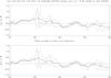 |
Fig. A.1
|
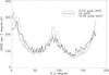 |
Fig. A.2 Histograms of the polarization orientation for the best y relative positioning of the two I + S and I − S spectra and for additional ± 0.25 pixels (± 1 arcsec) relative shifts. |
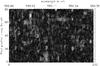 |
Fig. A.3 Mean |

First, line wings were used. True polarization is expected to be low in the wings.
After integration over time and space, the line wings polarization degree does not
exceed 0.4%. Therefore, the intensity gradient term may dominate the Stokes one. For
every slit position in all time sequences, we shifted one spectrum relative to the
other by ±0.25 pixels along the y direction, i.e. ±0.25 arcsec. The
resulting mean  and
and
 profiles are plotted in
Fig. A.1. They show a remaining non null polarization that exceeds the 0.4% maximum
amplitude in the absence of an imposed δy shift. Consequently, the
two I + S and
I − S 2D spectra’s relative positioning does not
need any correction. The 0.4% polarization degree maximum amplitude, observed in the
absence of additional δy shift, gives an estimate of the polarization
measurement noise.
profiles are plotted in
Fig. A.1. They show a remaining non null polarization that exceeds the 0.4% maximum
amplitude in the absence of an imposed δy shift. Consequently, the
two I + S and
I − S 2D spectra’s relative positioning does not
need any correction. The 0.4% polarization degree maximum amplitude, observed in the
absence of additional δy shift, gives an estimate of the polarization
measurement noise.
Building histograms of the line-center polarization-direction, orientation angular distribution is a second way to check the quality of the relativepositioning. On each side of an I(y) intensity peak, a relative shift in the y direction generates positive and negative intensity gradients and, therefore, radial and tangential polarizations. Consequently, a bad relative positioning of the two I + S and I − S spectra would generate two peaks at these perpendicular radial and tangential directions. As seen in Fig. A.2, shifting one spectrum relative to the other by ± 0.25 arcsec increases significantly the intensities of the polarization-direction orientation angular distribution function at θ = 0 and θ = 90. This, regardless the shift sign. Both these methods lead to the same conclusion; i.e., the observed polarization signal is not due to a bad relative positioning of the I + S and I − S 2D spectra.
Appendix A.3: V crosstalk
Significant V crosstalk requires a magnetic field of significant amplitude to be present at the observed location. V crosstalk does not play any role at line center, where impact polarization is observed. According to the magnetic field polarity, V crosstalk
should affect either the red or the blue wing. This contribution should be constant in time and position. Such time constant line-wing polarization enhancements are not observed. V crosstalk cannot explain the line-center strong polarization signals temporary observed.
Appendix A.4: Polarization fringes
Periodic structures in both the y and the wavelength directions are
present in THEMIS spectra (Semel 2003). The
false polarization signal that these fringes could introduce in the line 2D spectra,
is detectable by adding these spectra over time and over slit positions. For each
Stokes parameter, this leads to a mean Stokes S2D spectrum:
 The
resulting mean 2D polarization spectrum
The
resulting mean 2D polarization spectrum 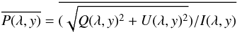 is
shown in Fig. A.3. This mean spectrum includes erroneous
is
shown in Fig. A.3. This mean spectrum includes erroneous
 contributions, due to a
few deficient couples of CCD pixels, and the contribution of the strongest
contributions, due to a
few deficient couples of CCD pixels, and the contribution of the strongest
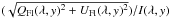 flare degrees of
polarization. Polarization fringes
flare degrees of
polarization. Polarization fringes  are the main contributors. They have amplitudes lower than 1%.
Fringes and CCD pixel default contributions to the Stokes polarization signal were
eliminated by subtracting mean  and
and  from all U/I and
Q/I 2D-spectra. In this
process, the noisy signal, expected to be constant over all the observing time, is
eliminated. Flare
UFl/I and
QFl/I Stokes
signals, present only during only nobs observations, are
marginally affected by this treatment. These Stokes signals are reduced by
nobs/(Ntime × Nslitpos),
where Ntime (= 12) and Nslitpos (=10) are
respectively the number of scans and the number of observations per scan. According on
the nobs value, this reduction factor does vary from 1 to
10%. Such a reduction does not significantly affect the flare linear polarization
measurements.
from all U/I and
Q/I 2D-spectra. In this
process, the noisy signal, expected to be constant over all the observing time, is
eliminated. Flare
UFl/I and
QFl/I Stokes
signals, present only during only nobs observations, are
marginally affected by this treatment. These Stokes signals are reduced by
nobs/(Ntime × Nslitpos),
where Ntime (= 12) and Nslitpos (=10) are
respectively the number of scans and the number of observations per scan. According on
the nobs value, this reduction factor does vary from 1 to
10%. Such a reduction does not significantly affect the flare linear polarization
measurements.
Acknowledgments
J. C. Hénoux wishes to thank the THEMIS team, Paris Observatory and the Laboratoire d’Etudes Spatiales et d’Instrumentation en Astrophysique (LESIA). This research was also supported by the grant P209/12/0103 (GA CR).
References
- Balança, C., & Dubois, A. 2001, 20th International Sacramento Peak Summer Workshop Advanced Solar Polarimetry, ed. M. Sigwarth, ASP Conf. Ser., 236 [Google Scholar]
- Bianda, M., Benz, A. O., Stenflo, J. O., Küveler, G., & Ramelli, R. 2005, A&A, 434, 11 [Google Scholar]
- Brosius, J. W. 2003, ApJ, 586, 1417 [NASA ADS] [CrossRef] [Google Scholar]
- Czaykowska, A., de Pontieu, B., Alexander, D., & Rank, G. 1999, ApJ, 521, 75 [Google Scholar]
- Fárník, F., Garcia, H., & Karlický, M. 2001, Sol. Phys., 201, 357 [NASA ADS] [CrossRef] [Google Scholar]
- Firstova, N. M., & Kashapova, L. K. 2002, A&A, 388, L17 [NASA ADS] [CrossRef] [EDP Sciences] [Google Scholar]
- Firstova, N. M., Hénoux, J.-C., Kazantsev, S. A., & Bulatov, A. V. 1997, Sol. Phys., 171, 12 [Google Scholar]
- Firstova, N. M., Xu, Z., & Fang, C. 2003, ApJ, 595, L131 [NASA ADS] [CrossRef] [Google Scholar]
- Firstova, N. M., Polyakov, V. I., & Firstova, A. V. 2005, Sol. Phys., 249, 53 [NASA ADS] [CrossRef] [Google Scholar]
- Fletcher, L., & Brown, J. C. 1998, A&A, 338, 737 [NASA ADS] [Google Scholar]
- Hanaoka, Y. 2003, ApJ, 596, 1347 [NASA ADS] [CrossRef] [Google Scholar]
- Hénoux, J.-C., & Karlický, M. 2003, A&A, 407, 1103 [NASA ADS] [CrossRef] [EDP Sciences] [Google Scholar]
- Hénoux, J.-C., & Semel, M. 1981, in Proc. Solar Maximum Workshop, eds. V. N. Obridko, & E. V. Ivanov (Moscow, Ismiran), 1, 207 [Google Scholar]
- Hénoux, J.-C., & Vogt, E. 1998, Phys. Scr., 78, 60 [CrossRef] [Google Scholar]
- Karlický, M. 2012, ApJ, 750, 49 [NASA ADS] [CrossRef] [Google Scholar]
- Karlický, M., & Hénoux, J.-C. 2002, A&A, 383, 713 [NASA ADS] [CrossRef] [EDP Sciences] [Google Scholar]
- Karlický, M., & Kosugi, T. 2004, A&A, 419, 1159 [NASA ADS] [CrossRef] [EDP Sciences] [Google Scholar]
- Kazantsev, S. A., & Henoux, J.-C. 1995, Polarization Spectroscopy of Ionized Gases (Dordrecht: Kluwer) [Google Scholar]
- Kleinpoppen, H. 1969, Physics of the One and Two-Electrons Atoms, eds. F. Bopp, & H. Kleinpoppen (Amsterdam: North-Holland), 612 [Google Scholar]
- Kleinpoppen, H., & Neugart, R. 1967, Z. Phys., 198, 321 [Google Scholar]
- Landi Degl’Innocenti, E., & Landolfi, M. 2004, Polarization in spectral lines (Dordrecht: Kluwer) [Google Scholar]
- Liu, R., & Wang, H. 2009, ApJ, 703, L23 [NASA ADS] [CrossRef] [Google Scholar]
- Metcalf, T., Wulzer, J.-P., Canfield, R., & Hudson, H. 1992, in the Compton Observatory Science Workshop, NASA Conf. Proc., 3137, 536 [Google Scholar]
- Metcalf, T., Mickey, D., Canfield, R., & Wulzer, J.-P. 1994, in High Energy Solar Phenomena, AIP Conf. Proc., 294, 59 [Google Scholar]
- Romano, P., Contarino, L., & Zuccarello, F. 2005, A&A, 433, 683 [NASA ADS] [CrossRef] [EDP Sciences] [Google Scholar]
- Semel, M. 2003, A&A, 401, 1 [NASA ADS] [CrossRef] [EDP Sciences] [Google Scholar]
- Somov, B. V., & Kosugi, T. 1997, ApJ, 485, 859 [NASA ADS] [CrossRef] [Google Scholar]
- Štěpán, J., Heinzel, P., & Sahal-Bréchot, S. 2007, A&A, 465, 621 [NASA ADS] [CrossRef] [EDP Sciences] [Google Scholar]
- Stumpf, B., Becker, K., & Schulz, G. 1978, J. Phys. B: At. Mol. Phys., 11, L639 [NASA ADS] [CrossRef] [Google Scholar]
- Vogt, E., & Hénoux, J.-C. 1996, Sol. Phys., 164, 345 [NASA ADS] [CrossRef] [Google Scholar]
- Vogt, E., & Hénoux, J.-C. 1999, A&A, 349, 283 [NASA ADS] [Google Scholar]
- Vogt, E., Sahal-Bréchot, S. & Hénoux, J.-C. 1997, A&A, 324, 1211 [NASA ADS] [Google Scholar]
- Vogt, E., Sahal-Bréchot, S., & Bommier, V. 2001, A&A, 374, 1127 [NASA ADS] [CrossRef] [EDP Sciences] [Google Scholar]
- Xu, Z., Hénoux, J.-C., Chambe, G., Karlický, M., & Fang C. 2005, ApJ, 631, 618 [NASA ADS] [CrossRef] [Google Scholar]
- Xu, Z., Hénoux, J.-C., Chambe, G., Petrashen, A. G., & Fang C. 2006, ApJ, 650, 1193 [NASA ADS] [CrossRef] [Google Scholar]
All Figures
|
Fig. 1 Radial polarization orientation generated by a vertical beam of particles moving
along vertical magnetic field lines. These particles are supposed to have velocities
close to the electron Na D2 collisional excitation threshold-velocity
|
| In the text | |
|
Fig. 2 Orientation, relative to the celestial north direction, N, of the axes used to define the Stokes parameters. OF indicates the Sun center to flare direction. ΘAR is the angle between this direction and the celestial north direction. |
| In the text | |
|
Fig. 3 2001 June 15 flare: GOES soft X-ray 1−8 A flux (dashed-dotted) in arbitrary units and HXRBS (Fárník et al. 2001) hard X-rays 19−29 keV (full line), 44−67 keV (dotted line) and 100−147 keV (dashed line) count rates. Vertical lines show times of observations presented in Figs. 4 and 6. |
| In the text | |
|
Fig. 4 Polarization pseudo-spectroheliograms of 2001 June 15th two-ribbon flare derived from four observing time sets. Intensity levels are in grey. y axis is labeled in arcsec. Each x axis label identifies a narrow 2D spectra in a set of eleven adjacent and successive 2D spectra of wavelength width 0.032 nm, covering 11 pixels. They correspond to scans made along the x direction (with a δx 2.5 arcsec scan step). Regions with Na D2 linear polarization degree higher than 3%, and with either tangential or radial polarization directions are in black or white. On the 10H 07M 20S pseudo-spectroheliogram, four letters, A, B, C, D, indicate locations where line intensity, polarization degree and orientation profiles were computed (see Fig. 5). |
| In the text | |
|
Fig. 5 Line intensity and line polarization degree spectral profiles (top) and line polarization orientation spectral profile (bottom), at locations A, B, C, and D (see Fig. 4). Dashed vertical lines give wavelength position of the Na D2 line, when solar rotation is taken into account. |
| In the text | |
|
Fig. 6 Number dN(θ) of pseudo-spectroheliograms pixels with polarization orientation equal to θ +/− one degree, as a function of θ. Three sets of pixels, with a polarization degree respectively higher than 6, 4, and 3%, have been selected. The associated histograms are drown in full, dashed, and dotted lines. |
| In the text | |
|
Fig. A.1
|
| In the text | |
|
Fig. A.2 Histograms of the polarization orientation for the best y relative positioning of the two I + S and I − S spectra and for additional ± 0.25 pixels (± 1 arcsec) relative shifts. |
| In the text | |
|
Fig. A.3 Mean |
| In the text | |
Current usage metrics show cumulative count of Article Views (full-text article views including HTML views, PDF and ePub downloads, according to the available data) and Abstracts Views on Vision4Press platform.
Data correspond to usage on the plateform after 2015. The current usage metrics is available 48-96 hours after online publication and is updated daily on week days.
Initial download of the metrics may take a while.