| Issue |
A&A
Volume 555, July 2013
|
|
|---|---|---|
| Article Number | L5 | |
| Number of page(s) | 4 | |
| Section | Letters | |
| DOI | https://doi.org/10.1051/0004-6361/201321620 | |
| Published online | 09 July 2013 | |
Fast-evolving weather for the coolest of our two new substellar neighbours
1 Institut d’Astrophysique et Géophysique, Université de Liège, allée du 6 Août 17, 4000 Liège, Belgium
e-mail: This email address is being protected from spambots. You need JavaScript enabled to view it.
2 Department of Physics, and Kavli Institute for Astrophysics and Space Research, Massachusetts Institute of Technology, Cambridge, MA 02139, USA
3 Observatoire de Genève, Université de Genève, 51 Chemin des Maillettes, 1290 Sauverny, Switzerland
Received: 1 April 2013
Accepted: 13 June 2013
Abstract
We present the results of intense photometric monitoring in the near-infrared (~0.9 μm) with the TRAPPIST robotic telescope of the newly discovered binary brown dwarf WISE J104915.57-531906.1, the third closest system to the Sun at a distance of only 2 pc. Our twelve nights of time-series photometry reveal a quasi-periodic (P = 4.87 ± 0.01h) variability with a maximum peak-peak amplitude of ~11% and strong night-to-night evolution. We attribute this variability to the rotational modulation of fast-evolving weather patterns in the atmosphere of the coolest component (~T1-type) of the binary. No periodic signal is detected for the hottest component (~L8-type). For both brown dwarfs, our data allow us to firmly discard any unique transit during our observations for planets ≥2 R⊕. For orbital periods smaller than ~9.5 h, transiting planets are excluded down to an Earth-size.
Key words: brown dwarfs / stars: individual: WISE-J104915.57-531906.1 / solar neighborhood / techniques: photometric
Fellow of the Swiss National Science Foundation.
© ESO, 2013
1. Introduction
The observational studies of brown dwarfs (BD) and exoplanets, both of which started in 1995 (Rebolo et al. 1995; Mayor & Queloz 1995), are two of the most active fields of modern astronomy. Notably, the atmospheric study of these substellar objects has seen tremendous advances recently, thanks to the sophistication of models and to the constant improvement of instruments (see e.g. Seager & Deming 2010; Kirckpatrick 2005; Showman & Kaspi 2012 for reviews). With effective temperatures ranging from ~300–2000 K, L, and T-types field BDs amenable for detailed direct studies represent critical precursors to the atmospheric characterization of giant exoplanets. The data gathered so far outline the important role of atmospheric condensates on the spectral morphologies of these objects (Kirckpatrick 2005). This is especially true at the L-T transition (~L7-T4 spectral types) that is characterized by an increase of the J-band luminosity with decreasing temperature (Vrba et al. 2004). This has been explained by the gradual depletion of silicates in the cooler atmospheres resulting in increasingly patchy cloud covers and thus increasingly small condensate opacity. Still, the details of this transition remain poorly understood (e.g. Saumon & Marley 2008). Most mechanisms put forward to explain the condensate depletion involve the fragmentation of the clouds (Ackerman & Marley 2001; Burgasser et al. 2002) driven by convection in the troposphere. They predict relatively large (~1–20%) photometric variability around 1μm on rotational timescales, driven by the constant formation, evolution, and complex dynamics of clouds clearing in the upper atmosphere.
Brown dwarfs are very rapid rotators (typically a few hours, Herbst et al. 2007), and this variability is observable within a few nights of photometric monitoring. Because of the extreme faintness in the optical at the L/T transition, only a handful of near-infrared (NIR) observations using medium-sized ground-based telescopes or space-based facilities could reach the photometric precision required to detect these predicted semi-periodic variabilities (Clarke et al. 2008; Artigau et al. 2009; Radigan et al. 2012; Khandrika et al. 2013; Apai et al. 2013). Overall, these results support a variant of the cloud fragmentation mechanism, with atmospheric patches of low opacity not entirely free of condensates. Still, there is no clear evidence yet that BDs at the L/T transition are drastically more variable than the other BDs (Khandrika et al. 2013). Additional high-precision photometric monitoring of L/T transition BDs is thus highly desirable. High-precision time-series photometry can also inform us of the spatial and temporal distribution of cloud structures, vertical thermal profiles, degrees of differential rotation, and of the age of brown dwarfs since their rotation period decreases monotonically with time.
A unique opportunity for this domain has come recently with the detection by Luhman (2013, hereafter L13) of a nearby binary BD at only 2.02 ± 0.15 pc. This system, WISE J104915.57-531906.1 (hereafter Luhman 16, following Mamajek 2013), is the third closest system to Earth, making it an exquisite target for high signal-to-noise ratio follow-up (J = 10.7, K = 8.8). With spectral types L8±1 for Luhman 16A and T1±2 for Luhman 16B (Kniazev et al. 2013, hereafter K13; see also Burgasser et al. 2013), both of its components lie within the L/T transition. This amazing system is an invaluable target for high-precision time-series photometry, an interest further reinforced by the classification of the pair as a possible variable in WISE All-Sky Source Catalog (L13). This motivated us to perform an intensive photometric monitoring of the system in the NIR using the 60cm robotic telescope TRAPPIST. We observed Luhman 16 for twelve nights, reaching a typical precision ~0.2% per bin of 10 min, thanks to the relatively large brightness of the system. This high precision allowed us to detect for the T-dwarf Luhman 16B a clear quasi-periodic variability combined with a fast evolution of the observed patterns.
The next section presents our TRAPPIST data and their reduction. Our analysis of the resulting photometric time series is described in Sect. 3. Finally, we discuss our results briefly in Sect. 4.
2. Data description
We monitored WISE 1049-5319 for twelve nights between 2013 March 14 and 26 with the robotic 60 cm telescope TRAPPIST (TRAnsiting Planets and Planetes Imals Small Telescope; Jehin et al. 2011) located at ESO La Silla Observatory in the Atacama Desert, Chile. The TRAPPIST telescope is equipped with a thermoelectrically-cooled 2 K × 2 K CCD having a pixel scale of 0.65′′ that translates into a 22′ × 22′ field of view. The observations were obtained with an exposure time of 115 s, with the telescope focused and through a special I + z filter having a transmittance >90% from 750 nm to beyond 1100 nm1. Considering the transmission curve of this I + z filter, the spectral response curve of the CCD detector, and the spectral type of the target, we derive an effective wavelength of ~910 nm for the observations. The positions of the stars on the chip were maintained to within a few pixels over the course of each run, thanks to a software guiding system that regularly derives an astrometric solution for the most recently acquired image and sends pointing corrections to the mount if needed.
After a standard pre-reduction (bias, dark, flatfield correction), the stellar fluxes for each run were extracted from the images using the IRAF/DAOPHOT2 aperture photometry software (Stetson 1987). The same photometric aperture of 8 pixels (~5.1′′) was used for all nights. After a careful selection of ten stable reference stars of similar brightness (|Δmag| < 1), differential photometry was then obtained. Finally, the light curves were normalized. The twelve resulting light curves are shown in Fig. 1. To assess the night-to-night variability of the target, we also extracted a global differential light curve that is shown in Fig. 2.
The typical full width at half maximum (FWHM) of the TRAPPIST point-spread function (PSF) is ~3 pixels = ~2′′. At this resolution, the two components of the 1.5′′ binary are only partially resolved, and our photometry extracted with an aperture of ~5.1′′ radius shows the evolution of the sum of the fluxes of both components.
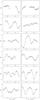 |
Fig. 1 Normalized TRAPPIST light curves for Luhman 16 binned per 10 min intervals. For each light curve, the best-fit global model (see Sect. 3) is over-imposed in red. Gaps for night #1 and #5 correspond to cloudy conditions. The gap for night #2 corresponds to the observation of another target. |
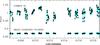 |
Fig. 2 Globally normalized TRAPPIST differential photometry for Luhman 16 (top) and for one of the comparison stars used in the reduction (bottom, shifted along the y-axis for the sake of clarity), unbinned (cyan) and binned per interval of 30 min (black). The standard deviation of the binned light curves are 2.2% and 0.1% for Luhman 16 and the comparison star, respectively. |
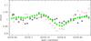 |
Fig. 3 Differential photometry for the second part of night 10, binned per 10 min intervals, obtained with an aperture encompassing both components of the binary (green filled circles), and with apertures encompassing only the PSF centre of Luhman 16A (black empty symbols) and Luhman 16B (red vertical bars). The variations are amplified on Luhman 16B, indicating that they originate from this T-dwarf. |
3. Data analysis
Although it is relatively stable on longer timescales (Fig. 2), Luhman 16 shows a clear variability on a nightly timescale (Fig. 1). Furthermore, the observed patterns evolve strongly from one night to the next. A Lomb-Scargle periodogram (Lomb 1976; Scargle 1982) applied to our photometry shows a strong power excess around ~0.2 d, matching well the typical separation between similar features in the light curves.
We performed a global analysis of our twelve light curves, adapting for that purpose the Markov chain Monte Carlo (MCMC) code described in Gillon et al. (2012, hereafter G12). In a first step, we assumed that the observed variability originated from only one of the two BDs. Elected by minimizing the Bayesian information criterion (BIC, Schwarz 1978), our model for the rotational modulation was based on a division of the brown dwarf into ten longitudinal slices. For each of them, the surface flux was assumed to be constant during each night, and the measured flux was modelled by a semi-sinusoidal function falling to zero when the slice disappeared from view. To this rotational model, we added a baseline model accounting for (i) the flip of the equatorial mount of the telescope at the meridian, putting the stellar images on different pixels and thus possibly creating small offsets in the differential photometry; (ii) a second-order airmass polynomial aiming to model the differential extinction curvature due to the much redder colour of the target compared to the comparison stars; and (iii) a fourth-order time polynomial representing the low-frequency variability of the system, including the evolution of the patterns from one rotation to the other. In this global model, the only two perturbed parameters in the MCMC were the rotation period and an arbitrary phase; the solution for the remaining parameters were obtained by linear regression at each step of the Markov chains (see G12 for details). Two MCMC chains of 100 000 steps were performed to probe the posterior distribution of the rotational period efficiently.
In the end, we obtained Prot = 4.87 ± 0.01 h, with an excellent fit between the model and the data (see Fig. 1). While a periodogram of the residuals reveals no additional period, we performed an additional analysis by adding a second rotational model to the MCMC. This analysis also failed to identify a second period. The BIC significantly increased by +360, indicating that a model including a single rotation period is a more likely representation of the data. We thus conclude that only one of the two BDs dominates the photometric variability since a same rotational period for both BDs is unlikely.
Aiming to determine which of the two BDs is the source of the observed variability, we performed a new photometric reduction of a fraction of our images with the IRAF/DAOPHOT ALLSTAR PSF-fitting software (Stetson 1987). This analysis allowed us to measure the T-dwarf to be 0.1 ± 0.1 mag brighter than the L-dwarf in our I + z filter, but failed to unambiguously determine which of the two was at the origin of the variability. At this stage, we tried another approach. Using only partial light curves corresponding to both the largest signal amplitudes and to the narrowest PSFs (FWHM ~ 1.5′′), we extracted the fluxes of both components by aperture photometry, fixing the aperture centres for the two BDs to two opposite positions on the line connecting their PSF centres on each side and at equal distance from the binary. The aperture sizes were then chosen to encompass only one PSF centre. For some light curves, a signal similar to the one shown in Fig. 1 but with a larger amplitude was clearly visible for the T-dwarf, while no light curve obtained for the L-dwarf showed any significant signal (e.g. Fig. 3). From these results, we conclude that the detected quasi-periodic variability originates from the T-dwarf Luhman 16B.
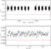 |
Fig. 4 Residuals of our global modelling, unfolded and binned per 10 min intervals (top), folded with P = 8 h and binned per 5 min intervals (bottom). For the unfolded residuals the expected transit depth for a 2 R⊕ planet orbiting one of the two BD is shown as a red horizontal line, assuming a 0.1 R⊙ radius and the same brightness for both BDs. The same is done for the folded residuals, but assuming a 1 R⊕ planet. |
4. Discussion
From their new spectroscopy and from the relationship of Stephens et al. (2009), K13 attribute to Luhman 16A and B components effective temperatures of 1350 ± 120 K and 1220 ± 110 K, respectively. These very low temperatures make atmospheric condensates the most likely source of the observed rotational variability (see discussion by Radigan et al. 2012, for the T1.5 BD 2M2139). The most surprising feature of the patterns reported here is their fast evolution from night to night. To our knowledge, this is the first time that such dramatic evolution is reported for the cloud coverage of an L/T transition BD, making Luhman 16B an actual Rosetta Stone for the study of BDs atmospheres. Future multi-band and high-cadence spectroscopic time series will be able to probe the spatial and spectral evolution of its cloud decks, giving unprecedented access into the physico-chemical processes acting in these atmospheres.
Considering our measured Δmag = 0.1 ± 0.1 between both BDs, the variability amplitudes visible in Fig. 1 are thus diluted by a factor of ~2 by the blend of both PSFs in the TRAPPIST images. The actual maximum peak-to-peak variability amplitude of Luhman 16B should thus be >20%. Similar amplitudes were observed around 1 μm for at least another early T-dwarf, the T1.5-type BD 2M2139 (Radigan et al. 2012). For the L-dwarf Luhman 16A, we do not detect any variability, but our sensitivity is limited by the partial resolution of both components in our images. High-cadence photometry with a better spatial resolution will be needed to thoroughly assess its photometric variability.
Field BDs are very interesting targets for exoplanets transit searches (Blake et al. 2008; Bolmont et al. 2011; Belu et al. 2013), as their small sizes make the detection of terrestrial planets possible with photometric precision at the mmag level similar to the ones reported here for Luhman 16. A careful visual inspection of the residual light curves and a search for periodic
box-like patterns with the BLS algorithm (Kovacs et al. 2002) failed to detect any transit-like signal. Despite the blend of both BDs, our sensitivity is good enough to partially probe the terrestrial regime. Figure 4 (top panel) shows the residuals of our global modelling for both BDs compared to the expected transit depths for a 2 R⊕ radius planet, assuming for each of them a 0.1 R⊙ radius. The corresponding transit is firmly discarded by our data. For orbital periods smaller than the mean duration of our runs (~9.5 h), our detection threshold goes down to Earth-sized planets, as can be seen in Fig. 4 (bottom panel). This shows that intensive campaigns like the one described here targeting the nearest field BDs with small to medium-sized ground-based telescopes or, even better, with an infrared space facility like Spitzer (Triaud et al., in prep.) could efficiently assess the frequency of close-in terrestrial planets around BDs, possibly detecting Earth-sized planets amenable for atmospheric characterization with the James Webb Space Telescope (JWST, Belu et al. 2013), for example.
IRAF is distributed by the National Optical Astronomy Observatory, which is operated by the Association of Universities for Research in Astronomy, Inc., under cooperative agreement with the National Science Foundation.
Acknowledgments
The authors thank Mark S. Marley, Adam J. Burgasser, and the anonymous referee for their valuable suggestions. TRAPPIST is a project funded by the Belgian Fund for Scientific Research (Fonds National de la Recherche Scientifique, F.R.S-FNRS) under grant FRFC 2.5.594.09.F, with the participation of the Swiss National Science Foundation (SNF). M. Gillon and E. Jehin are FNRS Research Associates. A.H. M. J. Triaud is Swiss National Science Foundation fellow under grant PBGEP2-145594. C. Opitom and L. Delrez thank the Belgian FNRS for funding their PhD theses.
References
- Ackerman, A. S., & Marley, M. S. 2001, ApJ, 556, 872 [NASA ADS] [CrossRef] [Google Scholar]
- Artigau, E., Bouchard, S., Doyon, R., & Lafrenière, D. 2009, ApJ, 701, 1534 [NASA ADS] [CrossRef] [Google Scholar]
- Apai, D., Radigan, J., Buenzli, E., et al. 2013, ApJ, 768, 121 [NASA ADS] [CrossRef] [Google Scholar]
- Belu, A. R., Selsis, F., Raymond, S. N., et al. 2013, ApJ, 768, 125 [NASA ADS] [CrossRef] [Google Scholar]
- Blake, C. H., Bloom, J. S., Latham, D. W., et al. 2008, PASP, 120, 860 [NASA ADS] [CrossRef] [Google Scholar]
- Bolmont, E., Raymond, S. N., & Leconte, J. 2011, A&A, 535, A94 [NASA ADS] [CrossRef] [EDP Sciences] [Google Scholar]
- Burgasser, A. J., Marley, M. S., Ackerman, A. S., et al. 2002, ApJ, 571, 151 [Google Scholar]
- Burgasser, A. J., Sheppard, S. S, & Luhman, K. L. 2013, ApJ, submitted [arXiv:1303.7283] [Google Scholar]
- Clarke, F. J., Hodgkin, S. T., Oppenheimer, B. R., et al. 2008, MNRAS, 386, 2009 [NASA ADS] [CrossRef] [Google Scholar]
- Gillon, M., Triaud, A. H. M. J., Fortney, J. J., et al. 2012, A&A, 542, A4 [NASA ADS] [CrossRef] [EDP Sciences] [Google Scholar]
- Herbst, W., Eislöffel, J., Mundt, R., & Scholz, A. 2007, Protostars and Planets V, eds. B. Reipurth, D. Jewitt, & K. Keil (Tucson: University of Arizona Press), 951, 297 [Google Scholar]
- Jehin, E., Gillon, M., Queloz, D., et al. 2011, The Messenger, 145, 2 [NASA ADS] [Google Scholar]
- Khandrika, H., Burgasser, A. J., Melis, C., et al. 2013, AJ, 145, 71 [NASA ADS] [CrossRef] [Google Scholar]
- Kirkpatrick, J. D. 2005, ARA&A, 43, 195 [NASA ADS] [CrossRef] [Google Scholar]
- Kniazev, A. Y., Vaisanen, P., Muzic, K., et al. 2013, ApJ, 770, 124 [NASA ADS] [CrossRef] [Google Scholar]
- Kovacs, G., Zucker, S., & Mazeh, T. 2002, A&A, 391, 369 [NASA ADS] [CrossRef] [EDP Sciences] [Google Scholar]
- Lomb, N. R. 1976, Ap&SS, 39, 447 [NASA ADS] [CrossRef] [Google Scholar]
- Luhman, K. L. 2013, ApJ, 767, L1 [NASA ADS] [CrossRef] [Google Scholar]
- Mamajek, E. E. 2013 [arXiv:1303.5345] [Google Scholar]
- Mayor, M., & Queloz, D. 1995, Nature, 378, 355 [NASA ADS] [CrossRef] [Google Scholar]
- Rebolo, R., Zapatero Osorio, M. R., & Martín, E. L. 1995, Nature, 377, 129 [NASA ADS] [CrossRef] [Google Scholar]
- Radigan, J., Jayawardhana, R., Lafrenière, D., et al. 2012, ApJ, 750, 105 [NASA ADS] [CrossRef] [Google Scholar]
- Saumon, D., & Marley, M. S. 2008, ApJ, 689, 1327 [NASA ADS] [CrossRef] [Google Scholar]
- Scargle, J. D. 1982, ApJ, 263, 835 [NASA ADS] [CrossRef] [Google Scholar]
- Schwarz, G. E. 1978, Annals of Statistics, 6, 461 [Google Scholar]
- Seager, S., & Deming, D. 2010, ARA&A, 48, 631 [NASA ADS] [CrossRef] [Google Scholar]
- Showman, A. P., & Kaspi, Y. 2012, ApJ, submitted [arXiv:1210.7573] [Google Scholar]
- Stephens, D. C., Leggett, S. K., Cushing, M. C., et al. 2009, ApJ, 702, 154 [NASA ADS] [CrossRef] [Google Scholar]
- Stetson, P. B. 1987, PASP, 99, 111 [Google Scholar]
- Vrba, F. J., Henden, A. A., Luginbuhl, C. B., et al. 2004, AJ, 127, 2948 [NASA ADS] [CrossRef] [Google Scholar]
All Figures
|
Fig. 1 Normalized TRAPPIST light curves for Luhman 16 binned per 10 min intervals. For each light curve, the best-fit global model (see Sect. 3) is over-imposed in red. Gaps for night #1 and #5 correspond to cloudy conditions. The gap for night #2 corresponds to the observation of another target. |
| In the text | |
|
Fig. 2 Globally normalized TRAPPIST differential photometry for Luhman 16 (top) and for one of the comparison stars used in the reduction (bottom, shifted along the y-axis for the sake of clarity), unbinned (cyan) and binned per interval of 30 min (black). The standard deviation of the binned light curves are 2.2% and 0.1% for Luhman 16 and the comparison star, respectively. |
| In the text | |
|
Fig. 3 Differential photometry for the second part of night 10, binned per 10 min intervals, obtained with an aperture encompassing both components of the binary (green filled circles), and with apertures encompassing only the PSF centre of Luhman 16A (black empty symbols) and Luhman 16B (red vertical bars). The variations are amplified on Luhman 16B, indicating that they originate from this T-dwarf. |
| In the text | |
|
Fig. 4 Residuals of our global modelling, unfolded and binned per 10 min intervals (top), folded with P = 8 h and binned per 5 min intervals (bottom). For the unfolded residuals the expected transit depth for a 2 R⊕ planet orbiting one of the two BD is shown as a red horizontal line, assuming a 0.1 R⊙ radius and the same brightness for both BDs. The same is done for the folded residuals, but assuming a 1 R⊕ planet. |
| In the text | |
Current usage metrics show cumulative count of Article Views (full-text article views including HTML views, PDF and ePub downloads, according to the available data) and Abstracts Views on Vision4Press platform.
Data correspond to usage on the plateform after 2015. The current usage metrics is available 48-96 hours after online publication and is updated daily on week days.
Initial download of the metrics may take a while.