| Issue |
A&A
Volume 555, July 2013
|
|
|---|---|---|
| Article Number | A61 | |
| Number of page(s) | 5 | |
| Section | Astronomical instrumentation | |
| DOI | https://doi.org/10.1051/0004-6361/201321295 | |
| Published online | 28 June 2013 | |
Expectation maximization for hard X-ray count modulation profiles
1
Dipartimento di MatematicaUniversità di Genova,
via Dodecaneso 35,
16146
Genova,
Italy
e-mail:
This email address is being protected from spambots. You need JavaScript enabled to view it.
2
Catholic University and Solar Physics Laboratory,
Goddard Space Flight Center, code
671, Greenbelt,
MD
20771,
USA
3
CNR – SPIN, via Dodecaneso 33, 16146
Genova,
Italy
Received:
14
February
2013
Accepted:
12
March
2013
Abstract
Context. This paper is concerned with the image reconstruction problem when the measured data are solar hard X-ray modulation profiles obtained from the Reuven Ramaty High Energy Solar Spectroscopic Imager (RHESSI) instrument.
Aims. Our goal is to demonstrate that a statistical iterative method classically applied to the image deconvolution problem is very effective when utilized to analyze count modulation profiles in solar hard X-ray imaging based on rotating modulation collimators.
Methods. The algorithm described in this paper solves the maximum likelihood problem iteratively and encodes a positivity constraint into the iterative optimization scheme. The result is therefore a classical expectation maximization method this time applied not to an image deconvolution problem but to image reconstruction from count modulation profiles. The technical reason that makes our implementation particularly effective in this application is the use of a very reliable stopping rule which is able to regularize the solution providing, at the same time, a very satisfactory Cash-statistic (C-statistic).
Results. The method is applied to both reproduce synthetic flaring configurations and reconstruct images from experimental data corresponding to three real events. In this second case, the performance of expectation maximization, when compared to Pixon image reconstruction, shows a comparable accuracy and a notably reduced computational burden; when compared to CLEAN, shows a better fidelity with respect to the measurements with a comparable computational effectiveness.
Conclusions. If optimally stopped, expectation maximization represents a very reliable method for image reconstruction in the RHESSI context when count modulation profiles are used as input data.
Key words: methods: statistical / techniques: image processing / Sun: flares / Sun: X-rays, gamma rays
© ESO, 2013
1. Introduction
Expectation maximization (EM; Dempster et al. 1977) is an iterative algorithm that addresses the maximum likelihood problem when 1) the relation between the unknown parameter (or set of parameters) and the measured data is linear; 2) the data are drawn from a Poisson distribution; 3) the unknown parameter satisfies the positivity constraint. EM represents a generalization of the image restoration method introduced by Lucy and Richardson Lucy (1974) for the deconvolution problems typical of focused astronomy, and it is successfully applied to several reconstruction problems in optics, microscopy and medical imaging. The present paper applies EM for the first time to the hard X-ray count modulation profiles measured by the nine rotating modulation collimators (RMCs) mounted on the Reuven Ramaty High Energy Solar Spectroscopic Imager (RHESSI; Lin et al. 2002). More specifically, we show here that, when combined with an optimal stopping rule for the iterative process, EM provides reliable reconstructions with notable computational effectiveness.
The RHESSI imaging concept translates the rotational modulation synthesis first introduced for non-solar observations to a solar context Hurford et al. (2002). In RHESSI, a set of nine rotating collimators, characterized by nine pairs of grids with nine different pitches, time-modulates the incoming photon flux before it is detected by the nine corresponding Ge crystals. The resulting signal is a set of nine time series representing the count evolution provided by each collimator-detector system at different time bins. Therefore, these count modulation profiles represent the temporal or rotation angle/phase variation of the count rates for each grid.
Since the transformation from the flux distribution on the image plane to the set of count modulation profiles is linear, the RHESSI image reconstruction problem is the linear inverse problem of describing the flux distribution from the count modulation profiles. EM describes the observed data and the unknown as realizations of stochastic quantities and then searches for the flux distribution that maximizes the probability of the observation under the constraint that the pixel content must be positive. In fact, when the noise distribution on the data is Poisson, this constrained maximum likelihood problem can be transformed into a fixed point problem whose solution is obtained iteratively by means of a successive approximation scheme. From a theoretical viewpoint, the convergence properties of this algorithm when the number of iterations grows are not completely known. However, it is always observed in applications that stopping the procedure at some optimal iteration regularizes the reconstruction, thus preventing the occurrence of over-resolving effects or short-wavelength artifacts. In this paper, this optimized stopping rule is determined by utilizing the concept of constrained residual and by imposing that the empirical expectation value of this stochastic variable coincides with its theoretical expectation value.
The plan of the paper is as follows. In Sect. 2 we describe the RHESSI imaging concept in more detail and introduce the linear transformation modeling the data formation process. Section 3 contains the formulation of the iterative algorithm, together with its stopping rule. Section 4 validates EM in the case of several synthetic modulation profiles simulated from plausible configurations of the flux distribution. Finally, in Sect. 5 we consider the application of EM to three sets of observed RHESSI data. Our conclusions are in Sect. 6.
2. RHESSI count modulation profiles
The RHESSI imaging hardware is made of nine subcollimators, each one consisting of a pair
of separated grids in front of a hard X-ray/gamma-ray detector. In each subcollimator the
two grids are identical and parallel and are characterized by a planar array of
equally-spaced, X-ray-opaque slats separated by transparent slits. The grid pitches of the
different collimators are arranged according to a geometric progression with factor
 ,
with detector 1 providing the maximum resolution power and minimum signal-to-noise ratio and
detector 9 providing the minimum resolution power and maximum signal-to-noise ratio. RHESSI
rotates around its own axis with a period of around 4 s and this rotation, combined with the
presence of the grids, induces the modulation of the count rates. Therefore in this
framework, there is no detector plane containing physical pixels (as in focused imaging) and
here pixels are just a mathematical idealization in the image reconstruction process. If we
describe the brightness distribution by means of the vector f of dimension
N2 × 1 (in this lexicographic ordering each vector index
denotes one of the N2 pixels), then the expected count
modulation detected by subcollimator l is given by
,
with detector 1 providing the maximum resolution power and minimum signal-to-noise ratio and
detector 9 providing the minimum resolution power and maximum signal-to-noise ratio. RHESSI
rotates around its own axis with a period of around 4 s and this rotation, combined with the
presence of the grids, induces the modulation of the count rates. Therefore in this
framework, there is no detector plane containing physical pixels (as in focused imaging) and
here pixels are just a mathematical idealization in the image reconstruction process. If we
describe the brightness distribution by means of the vector f of dimension
N2 × 1 (in this lexicographic ordering each vector index
denotes one of the N2 pixels), then the expected count
modulation detected by subcollimator l is given by  (1)where the vector
g(l) has dimensions
P(l) × 1,
P(l) is the number of time bins
discretizing the time evolution of the modulation for detector l and
H(l) with dimension
P(l) × N2, is
the matrix modeling the transformation from the image to the measurement space. The entries
of H(l) can be interpreted in a probabilistic way
as
(1)where the vector
g(l) has dimensions
P(l) × 1,
P(l) is the number of time bins
discretizing the time evolution of the modulation for detector l and
H(l) with dimension
P(l) × N2, is
the matrix modeling the transformation from the image to the measurement space. The entries
of H(l) can be interpreted in a probabilistic way
as 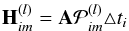 (2)where
A measures the detector area and
(2)where
A measures the detector area and  is the
probability that a photon originating in pixel m will be counted in the
ith time bin of detector l during the time interval
△ ti. If the image analysis performed
involves data collected by M of the nine subcollimators, then the overall
signal formation process is described by
is the
probability that a photon originating in pixel m will be counted in the
ith time bin of detector l during the time interval
△ ti. If the image analysis performed
involves data collected by M of the nine subcollimators, then the overall
signal formation process is described by  (3)where g has
dimensions L × 1,
(3)where g has
dimensions L × 1,  and
contains all the modulation profiles, while H has dimensions
L × N2 and represents the image operator
mimicking the action of the telescope. The EM algorithm, together with its optimal stopping
rule, provides an estimate of f by means of an iterative regularized inversion
of H.
and
contains all the modulation profiles, while H has dimensions
L × N2 and represents the image operator
mimicking the action of the telescope. The EM algorithm, together with its optimal stopping
rule, provides an estimate of f by means of an iterative regularized inversion
of H.
3. The EM algorithm
Expectation maximization is a statistical algorithm maximizing the probability that the
data vector is a realization corresponding to a Poisson random vector g. In
fact, in this case, the likelihood, i.e. the probability to observe g from
the model Hf, can be written as  (4)where the ratio
should be intended point-wise, element by element. We observe that maximizing this
probability corresponds to minimizing the Cash statistic (C-statistic; Cash 1979)
(4)where the ratio
should be intended point-wise, element by element. We observe that maximizing this
probability corresponds to minimizing the Cash statistic (C-statistic; Cash 1979)  (5)The likelihood maximizer is
constrained to the set of positive solutions; i.e., the algorithm solves the constrained
optimization problem
(5)The likelihood maximizer is
constrained to the set of positive solutions; i.e., the algorithm solves the constrained
optimization problem  (6)which can be
transformed into a fixed-point problem solved by means of the successive approximation
scheme
(6)which can be
transformed into a fixed-point problem solved by means of the successive approximation
scheme  (7)with a positive
(constant) initialization and where 1 denotes the vector made of all unit entries (in this
equation and in the following ones, products and ratios must be considered component-wise).
Since H is ill-conditioned, this iterative algorithm should be regularized by
applying some stopping rule. To this aim we observe that the asymptotical behavior of Eq.
(7) is such that either
fk → 0 or
(7)with a positive
(constant) initialization and where 1 denotes the vector made of all unit entries (in this
equation and in the following ones, products and ratios must be considered component-wise).
Since H is ill-conditioned, this iterative algorithm should be regularized by
applying some stopping rule. To this aim we observe that the asymptotical behavior of Eq.
(7) is such that either
fk → 0 or  (8)converges
to 1. This implies that, asymptotically,
(8)converges
to 1. This implies that, asymptotically,  (9)tends
to zero, and therefore a reasonable stopping rule for EM in the RHESSI case is
(9)tends
to zero, and therefore a reasonable stopping rule for EM in the RHESSI case is  (10)where
E(zk) denotes the
expectation value of zk.
(10)where
E(zk) denotes the
expectation value of zk.
4. Numerical validation
In order to assess the reliability of EM we setup a validation test based on the following process:
-
1.
Five different configurations of the flaring region were in-vented (see Fig. 1), with the first row characterizedby very different topographical and physical properties (e.g.,size, position, number and distance of disconnected compo-nents, or relative intensity of the components). Specifically, theoriginal configurations are a line source with constant densityalong the line (case A); a line source with intensity varying alongthe line, i.e. four compact sources and a weak one, all sourcesbeing aligned (case B); two Gaussian sources with flux ratio equalto 1 (case C); two Gaussian sources with flux ratio equal to 5 (caseD); two Gaussian sources with flux ratio equal to 10 (case E);
-
2.
For each flaring configuration, three different synthetic sets of count modulation profiles were realized, characterized by three different levels of statistics (low, medium, high). Operationally, matrix H was applied to the simulated map, the resulting count expected values at each time bin were scaled with three different values to simulate three different levels of statistics (an average of 1000 counts per detector for the low level, 10 000 for the medium level and 100 000 for the high one);
-
3.
EM was applied to each one of the resulting 15 data sets in order to reconstruct the images;
-
4.
A set of routines was applied for the quantitative assessment of the algorithm performance. These routines compute specific physical and geometrical parameters in the images, which are particularly significant for the different configurations, and compare the values with the corresponding ground truth values in the simulation maps of Fig. 1, first row.
Rows 2 through 4 of Fig. 1 contain the reconstructions provided by EM for the three different levels of statistics and use the count modulation profiles provided by all nine RHESSI detectors. The assessment routines are applied to these maps and compute the following parameters.
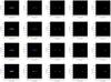 |
Fig. 1 Validation of EM with synthetic data. First row: the simulated configurations. Rows 2 through 4: reconstructions provided by EM corresponding to count modulation profiles characterized by three different levels of statistics (second row: average of 100 000 counts per detector; third row: average of 10 000 counts per detector; fourth row: average of 1000 counts per detector. |
Case A (line source with constant intensity):
-
A1: orientation (ground truth: 0 deg).
-
A2: number of reconstructed sources (ground truth: 1). While reconstructing a line source, most (if not all) imaging methods tend to break it up into a set of compact sources (this occurs particularly at low levels of statistics). The routine computes the number K of intersection knots between the reconstructed line profile and the straight line with the same orientation passing through the full width at half maximum (FWHM). The number of reconstructed sources is counted as K/2.
-
A3: length (ground truth: 20.2 arcsec). The routine computes the FWHM in the direction of the orientation line.
-
A4: width (ground truth: 1.35 arcsec). The routine computes the FWHM in the direction orthogonal to the orientation line.
Case B (line source with intensity varying along the line)
-
B1: orientation (ground truth: 0 deg).
-
B2: number of reconstructed sources at FWHM (ground truth: 4). Computed as in case A2.
-
B3: length (ground truth: 16.9 arcsec). Computed as in case A3.
-
B4: width (ground truth: 1.35 arcsec). Computed as in case A4.
-
C1: position of the first reconstructed source (ground truth: 0 arcsec). The routine computes the distance between the peak of the first reconstructed source and the corresponding simulated one.
-
C2: position of the second reconstructed source (ground truth: 0 arcsec). The routine computes the distance between the peak of the second reconstructed source and the corresponding simulated one.
-
C3: separation of the reconstructed sources (ground truth: 20 arcsec). The routine computes the distance between the two peaks.
-
C4: orientation of the separation line (ground truth: 0 deg). The routine computes the orientation of the line passing through the two reconstructed peaks.
-
C5: flux ratio (ground truth: 1). For each simulated source, the routine computes the disk centered on the correspondence with the peak and the radius such that 99% of the flux is within the disk. Then, in the reconstructed image, the routine computes the fluxes contained in the two disks and computes the ratio.
For Case D (two sources with flux ratio 5) and Case E (two sources with flux ratio 10) the routines compute the same parameters as in Case C.
We performed this analysis by comparing the parameters obtained by EM with the original simulation parameters and with the ones obtained by different imaging algorithms, namely: Pixon (Puetter 1995; Metcalf et al. 1996), CLEAN (Högbom 1974), Maximum Entropy (Bong et al. 2006), a forward-fit algorithm for visibilities and uv_smooth (Massone et al. 2009) (for all algorithms we used all nine RHESSI detectors). In Table 1 we reported just the results provided by Pixon, since among the methods using modulation profiles as input, it provided among the best results. The Pixon algorithm models the source as a superposition of circular sources (or pixons) of different sizes and parabolic profiles and looks for the one that best reproduces the measured modulations from the different detectors. This technique is generally considered to be the most reliable one in providing the most accurate image photometry (Dennis & Pernack 2009), but at the price of a very notable computational burden. In this experiment we configured the Pixon algorithm in Solar SoftWare (SSW) according to an optimized procedure based on heuristic arguments.
Assessment of EM and Pixon performances for synthetic data.
5. Application to real observations
We applied EM to RHESSI observations recorded in correspondence with three real flaring events. We considered the 2002 April 15 flare in the time interval 00:06:00−00:08:00 UT and in the energy interval 12−14 keV; the 2002 February 20 flare in the time interval 11:05:58−11:06:41 UT and in the energy interval 25−30 keV; the 2002 July 23 flare in the time interval 00:30:00−00:32:00 UT and in the energy interval 100−300 keV. In all cases detectors 3 through 8 are used for the observations. The reasons for this choice are as follows. Detector 2 has been characterized by malfunctions since the beginning of the RHESSI mission, detector 1 is characterized by a very small signal-to-noise ratio while the coarse information carried by detector 9 is not crucial for reconstructing these events. Figure 2 compares EM reconstructions with the ones provided by Pixon and CLEAN, while Table 2 contains the corresponding C-statistic for the six detectors employed in the analysis. In these experiments CLEAN parameters have been chosen according to optimized heuristic recipes (Dennis & Pernack 2009). According to these results, EM and Pixon are characterized by values of the C-statistic almost systematically close to 1 (and significantly lower than the ones provided by CLEAN). This means the EM and Pixon can reproduce the data with comparable accuracy (significantly better than the one achieved by CLEAN), although EM reduces the computational time of up to a factor 4. Indeed, for April 15, 2002, the computational time is around 100 s for EM and more than 400 s for Pixon; for February 20, 2002, the computational time is around 50 s for EM and almost 220 s for Pixon; for July 23, 2002, the computational time is around 125 s for EM and more than 460 s for Pixon. This same 4-to-1 scaling holds true independently of the kind of hardware used for the tests. We also observe that in the Pixon implementation we used for these experiments the computations of the time profiles and back projections are done more efficiently by using optimized combinations of the spatial variation as spatial sine and cosine patterns (annsec, annular-sector, implementation). Implementing EM according to this same representation will improve the computational gain provided by this algorithm of another factor 5.
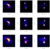 |
Fig. 2 Performance of EM with real data observed by RHESSI. First row: EM reconstructions; second row: Pixon reconstructions; third row: CLEAN reconstructions. First column: 15 April 2002 event; second column: 20 February 2002 event; third column: July 23 2002 event. |
Performance of EM with real data observed by RHESSI: comparisons of C-statistic provided by EM, Pixon and CLEAN.
6. Conclusions
This papers shows that expectation maximization can be effectively applied to reconstruct hard X-ray images of solar flares from the count modulation profiles recorded by the RHESSI mission. This method is an iterative likelihood maximizer with a positivity constraint, which explicitly exploits that the noise affecting the measured data is Poissonian. We utilized an optimal stopping rule that regularizes the algorithm, achieving an optimal trade-off between the C-statistic and the numerical stability of the reconstruction. We are aware that this test of the C-statistic is not conclusive, since images affected by significant artifacts may reproduce the experimental data with high accuracy; however, low C-statistic values coupled with the positivity constraint can be considered as a diagnostic of reliable reconstructions.
We validated EM against synthetic count modulation profiles corresponding to challenging simulated configurations and characterized by three levels of statistics. Then we applied the method against the RHESSI observations of three flaring events and compared the reconstructions with the ones provided by Pixon and CLEAN. The results of these experiments show that EM combines a reconstruction fidelity (in terms of C-statistic) comparable to the one provided by Pixon (which, however, is much more demanding from a computational viewpoint) with a computational efficiency comparable to the one offered by CLEAN (which, however, predicts the count modulation profiles by means of a significantly worse C-statistic). Our next step, which is currently under construction, will be to generalize this approach to the reconstruction of electron flux maps of the flaring region. Electron flux maps of solar flares can already be generated by hard X-ray count visibilities (Piana et al. 2007). We are currently working on an EM-based approach to the reconstruction of electron images, where the input data are the count modulation profiles and the imaging matrix to invert accounts for both the effects of the bremsstrahlung cross-section and the Detector Response Matrix mimicking the projection from the photon to the count domain. The advantage of this approach over the visibility-based one should be that EM provides an analysis framework that is closer to the data, because we can model all of the detector effects with higher accuracy.
Acknowledgments
The experiment with synthetic data in Sect. 4 was conceived in collaboration with A. G. Emslie and G. H. Hurford, who are kindly acknowledged. This work was supported by the European Community Framework Program 7, “High Energy Solar Physics Data in Europe (HESPE)”, Grant Agreement No. 263086.
References
- Bong, S. C., Lee, J., Gary, D. E., & Yun, H. S. 2006, ApJ, 636, 1159 [NASA ADS] [CrossRef] [Google Scholar]
- Cash, W. 1979, ApJ, 228, 939 [NASA ADS] [CrossRef] [Google Scholar]
- Dempster, A. P., Laird, N. M., & Rubin, D. B. 1977, J. Roy. Stat. Soc. B, 39, 1 [Google Scholar]
- Dennis, B. R., & Pernak, R. L. 2009, ApJ, 698, 2131 [NASA ADS] [CrossRef] [Google Scholar]
- Lucy, L. B. 1974, AJ, 79, 745 [NASA ADS] [CrossRef] [Google Scholar]
- Lin, R. P., Dennis, B. R., Hurford, G. J., et al. 2002, Sol. Phys., 210, 3 [Google Scholar]
- Högbom, J. A. 1974, A&A, 15, 417 [Google Scholar]
- Hurford, G. J. 2002, Sol. Phys., 210, 61 [NASA ADS] [CrossRef] [Google Scholar]
- Massone, A. M., Emslie, A. G., Hurford, G. J., Kontar, E. P., & Piana, M. 2009, ApJ, 703, 2004 [NASA ADS] [CrossRef] [Google Scholar]
- Metcalf, T. R., Hudson, H. S., Kosugi, T., Puetter, R. C., & Pina, R. K. 1996, ApJ, 466, 585 [NASA ADS] [CrossRef] [Google Scholar]
- Piana, M., Massone, A. M., Hurford, G. J., et al. 2007, ApJ, 665, 846 [Google Scholar]
- Puetter, R. C. 1995, Int. J. Image Sys. & Tech., 6, 314 [CrossRef] [Google Scholar]
All Tables
Performance of EM with real data observed by RHESSI: comparisons of C-statistic provided by EM, Pixon and CLEAN.
All Figures
|
Fig. 1 Validation of EM with synthetic data. First row: the simulated configurations. Rows 2 through 4: reconstructions provided by EM corresponding to count modulation profiles characterized by three different levels of statistics (second row: average of 100 000 counts per detector; third row: average of 10 000 counts per detector; fourth row: average of 1000 counts per detector. |
| In the text | |
|
Fig. 2 Performance of EM with real data observed by RHESSI. First row: EM reconstructions; second row: Pixon reconstructions; third row: CLEAN reconstructions. First column: 15 April 2002 event; second column: 20 February 2002 event; third column: July 23 2002 event. |
| In the text | |
Current usage metrics show cumulative count of Article Views (full-text article views including HTML views, PDF and ePub downloads, according to the available data) and Abstracts Views on Vision4Press platform.
Data correspond to usage on the plateform after 2015. The current usage metrics is available 48-96 hours after online publication and is updated daily on week days.
Initial download of the metrics may take a while.