| Issue |
A&A
Volume 555, July 2013
|
|
|---|---|---|
| Article Number | A26 | |
| Number of page(s) | 8 | |
| Section | Galactic structure, stellar clusters and populations | |
| DOI | https://doi.org/10.1051/0004-6361/201321183 | |
| Published online | 21 June 2013 | |
M• − σrelation for intermediate-mass black holes in globular clusters
1 European Southern Observatory (ESO), Karl-Schwarzschild-Strasse 2, 85748 Garching, Germany
e-mail: nluetzge@eso.org
2 Gemini Observatory, Northern Operations Center, 670 N. A’ohoku Place Hilo, Hawaii, 96720, USA
3 School of Mathematics and Physics, University of Queensland, Brisbane, QLD 4072, Australia
4 Instituto de Astronomia, Universidad Nacional Autonoma de Mexico (UNAM), A.P. 70-264, 04510 Mexico, Mexico
5 University Observatory, Ludwig Maximilians University, 81679 Munich, Germany
6 Sterrewacht Leiden, Leiden University, Postbus 9513, 2300 RA Leiden, The Netherlands
7 Astronomy Department, University of Texas at Austin, Austin, TX 78712, USA
8 I.Physikalisches Institut, Universität zu Köln, Zülpicher Str. 77, 50937 Köln, Germany
Received: 29 January 2013
Accepted: 26 April 2013
Context. For galaxies hosting supermassive black holes (SMBHs), it has been observed that the mass of the central black hole (M•) tightly correlates with the effective or central velocity dispersion (σ) of the host galaxy. The origin of this M• − σ scaling relation is assumed to lie in the merging history of the galaxies, but many open questions about its origin and the behavior in different mass ranges still need to be addressed.
Aims. The goal of this work is to study the black-hole scaling relations for low black-hole masses, where the regime of intermediate-mass black holes (IMBHs) in globular clusters (GCs) is entered.
Methods. We collected all existing reports of dynamical black-hole measurements in GCs, providing black-hole masses or upper limits for 14 candidates. We plotted the black-hole masses versus different cluster parameters including total mass, velocity dispersion, concentration, and half-mass radius. We searched for trends and tested the correlations to quantify their significance using a set of different statistical approaches. For correlations with a high significance we performed a linear fit, accounting for uncertainties and upper limits.
Results. We find a clear correlation between the mass of the IMBH and the velocity dispersion of the GC. As expected, the total mass of the GC then also correlates with the mass of the IMBH. While the slope of the M• − σ correlation differs strongly from the one observed for SMBHs, the other scaling relations M• − Mtot, and M• − L are similar to the correlations in galaxies. Significant correlations of black-hole mass with other cluster properties were not found in the present sample.
Key words: black hole physics / stars: kinematics and dynamics
© ESO, 2013
1. Introduction
Empirical scaling relations between the masses of nuclear black holes and properties of their host galaxies in terms of total luminosity L, bulge mass Mbulge (Kormendy & Richstone 1995; Marconi & Hunt 2003; Häring & Rix 2004) or the effective (projected) velocity dispersion σ (Ferrarese & Merritt 2000; Gebhardt et al. 2000a; Ferrarese & Ford 2005; Gültekin et al. 2009) disclose a strong connection between the formation history of supermassive black holes (SMBHs) and galaxies. These scaling relations can be explained by gas-accreting black holes that drive powerful jets and outflows into the surrounding interstellar medium, thus affecting the star formation rate and regulating the subsequent supply of matter onto the SMBH (Silk & Rees 1998; Di Matteo et al. 2005; Springel et al. 2005; Hopkins et al. 2007). Alternative explanations reproduce these empirical correlations by large numbers of merger events in which extreme values of M• / Mbulge are averaged out.
While galaxies and central SMBHs in the most common mass range, , seem to closely follow the one-parameter power law M• − σ and M• − L relations, there is now some evidence for large scatter or an upward curvature trend for SMBH masses at the highest mass regime (, e.g. Gebhardt et al. 2011; McConnell et al. 2011; van den Bosch et al. 2012; Hlavacek-Larrondo et al. 2012).
Given this puzzling behavior of the M• − σ relation at high masses, the question arises if different laws apply for the low-mass end as well. Attempts of measuring lower black-hole masses in dwarf galaxies (e.g. Filippenko & Ho 2003; Barth et al. 2004; Xiao et al. 2011) sparsely populate the relation down to a black-hole mass of ~105, but not lower. The lower the black-hole mass, the fainter they appear in radio and X-ray emission and the weaker is the kinematic signature and the smaller the radius of influence. Therefore, detecting black-hole masses lower than 105 M⊙ is challenging. Reaching for the mass range that currently is assigned to intermediate-mass black holes (IMBHs, 102 − 105 M⊙) requires extending the search toward different stellar systems.
The possible existence of IMBHs in low-mass stellar systems such as globular clusters (GCs) was first suggested by Silk & Arons (1975) while studying X-ray sources in a large sample of GCs. These authors concluded that the observed X-ray fluxes could only be explained by mass accretion onto a 100 − 1000 M⊙ central black hole. This discovery triggered a burst of black-hole hunting in GCs using X-ray and radio emission but also photometric and kinematic signatures.
Owing to the small amount of gas and dust in GCs, the accretion efficiency of a potential black hole at the center is expected to be low. This makes the detection of IMBHs at the centers of GCs through X-ray and radio emissions very challenging (Miller & Hamilton 2002; Maccarone & Servillat 2008). However, several attempts were made to detect radio and X-ray emission of gas in the central regions and to provide a black-hole mass estimate (e.g. Maccarone et al. 2005; Ulvestad et al. 2007; Bash et al. 2008; Cseh et al. 2010). Recently, Strader et al. (2012) tested several Galactic GCs for the presence of possible IMBHs by investigating radio and X-ray emission. They only found upper limits on the order of 102 M⊙. However, the authors had to make various assumptions about the gas accretion process such as gas distribution, accretion efficiency, and transformation of X-ray fluxes to black-hole masses to derive those limits. Besides X-ray and radio emission, the central kinematics in GCs can reveal possible IMBHs.
Motivated by the results of Silk & Arons (1975), Bahcall & Wolf (1976) claimed the detection of an IMBH in M15 by measuring its light profile and comparing it with dynamical models. The first claim from kinematic measurements was made by Peterson et al. (1989), who found a strong rise in the velocity dispersion profile of M15. More recently, Gebhardt et al. (1997, 2000b) and Gerssen et al. (2002) estimated a black-hole mass in M15 of (3.2 ± 2.2) × 103 M⊙ from photometric and kinematic observations. However, after more investigations this cluster no longer appears as a strong IMBH hosting candidate (e.g. Dull et al. 1997; Baumgardt et al. 2003, 2005; van den Bosch et al. 2006) and the previously detected X-ray sources turned out to be a large number of low-mass X-ray binaries, but new detections of IMBH candidates in other clusters followed.
Using integrated light near the center of the M31 cluster G1, Gebhardt et al. (2002, 2005) measured the velocity dispersion of this cluster and argued for the presence of a (1.8 ± 0.5) × 104 M⊙ IMBH. Furthermore, X-ray and radio emission were detected at the cluster center, consistent with a black hole of the same mass (Pooley & Rappaport 2006; Kong 2007; Ulvestad et al. 2007). This result, however, was recently challenged by Miller-Jones et al. (2012), who found no radio signature at the center of G1 when repeating the observations.
Another good candidate for hosting an IMBH at its center is the massive GC ω Centauri (NGC 5139). Noyola et al. (2008, 2010) measured the velocity-dispersion profile with an integral-field unit and used dynamical models to analyze the data. Because of the distinct rise in the velocity-dispersion profile they claimed a black-hole mass of M• = 40 000 M⊙. The same object was studied by Anderson & van der Marel (2010) using proper motions from Hubble Space Telescope (HST) images. They found less compelling evidence for a central black hole, but more importantly, they found a location for the center that differs from previous measurements. Both G1 and ω Centauri have been suggested to be stripped nuclei of dwarf galaxies (Freeman 1993; Meylan et al. 2001; Jalali et al. 2012) and therefore may not be the best representatives of GCs.
Further evidence for the existence of IMBHs is provided by the discovery of ultra-luminous X-ray (ULX) sources at non-nuclear locations in starburst galaxies (e.g. Fabbiano 1989; Colbert & Mushotzky 1999; Matsumoto et al. 2001; Fabbiano et al. 2001). The brightest of these compact objects (with L ~ 1041 erg s-1) imply masses larger than 103 M⊙ assuming no beaming of the X-ray emission and accretion at the Eddington limit. Probably one of the best IMBH candidates, the ULX source HLX-1, was discovered in an off-center position of the spiral galaxy ESO243-49 by Farrell et al. (2009) and Godet et al. (2009) and is most likely associated with a group of young stars remaining from the core of a stripped dwarf galaxy (e.g. Soria et al. 2010, 2013).
Properties of the 14 GCs of our sample.
In this paper we take the latest results for IMBH measurements in GCs from the literature and search for correlations with properties of their host cluster. For the first time, enough datapoints on IMBHs are available to perform this analysis. Established relations for SMBHs and their host galaxies, such as the M• − σ relation or the M• − Mtot, are the focus of this work. Probing the low-mass end of these correlations will provide important information about the origin and growth of SMBHs. In Sect. 2 we introduce the sample and the data from the literature used in this work. Section 3 describes the methods we applied for determining correlation coefficients and regression parameters, and in Sect. 4 we discuss the main correlations and their statistical significance. Finally, Sect. 5 summarizes our work and lists our conclusions.
2. The sample
The sample we chose for our analysis consists of 14 Galactic GCs for which we have kinematic measurements of their central regions. The majority of these measurements come from integral-field spectroscopy and were carried out by our group (Lützgendorf et al. 2011, 2012, 2013).
These clusters were observed with the GIRAFFE spectrograph of the Fiber Large Array Multi Element Spectrograph (FLAMES, Pasquini et al. 2002) instrument at the Very Large Telescope (VLT) using the ARGUS mode (large integral field unit). The velocity-dispersion profile was obtained by combining the spectra in radial bins centered around the adopted photometric center and measuring the broadening of the lines using a non parametric line-of-sight velocity-distribution fitting algorithm. For larger radii, the kinematic profiles were completed with radial velocity data from the literature, when available. In addition to the spectroscopic data, HST photometry was used to obtain the star catalogs, the photometric center of the cluster, and its surface brightness profile. For each cluster photometry and spectroscopy were combined to apply analytic Jeans models to the data. The surface brightness profile was used to obtain a model velocity-dispersion profile that was fit to the data by assuming different black-hole masses and M / LV profiles. The final black-hole masses were obtained from a χ2 fit to the kinematic data. Table 1 lists all clusters of the sample and their main properties.
In four clusters of our sample we found signatures of an IMBH. These clusters are NGC 6388, NGC 6266, NGC 1904, and NGC 5286. All of them show a rise in the velocity dispersion and require black-hole masses between 1.5 × 10³ − 2 × 10⁴ M⊙. A high radial anisotropy in the center of these clusters would also explain the rise in the velocity-dispersion profile. However, N-body simulations have shown that any anisotropy in the center of a GC would be smoothed out after several of relaxation times (Lützgendorf et al. 2011). Since all these clusters are older than at least 5−10 relaxation times, we conclude that the best explanation for the rise of the kinematic profile is indeed a black hole. Nevertheless, the result of the cluster NCG 1904 has to be treated carefully since the rise might occur from a mismatch of outer and inner kinematics. The rest of the clusters in our sample shows less evidence for a central black hole with shallow or even dropping velocity-dispersion profiles. For these we adopted the 1σ errors of the measurement as the upper limit.
ωCentauri, G1, and NGC 6715 are GCs with measured black-hole masses not obtained by our group. For ω Centauri we used the latest result of Noyola et al. (2010) for the black-hole mass of the IMBH in ω Centauri of ~47 000 M⊙, which was derived by studying VLT/FLAMES integral-field spectroscopy data of the inner kinematics, similar to the method described above. This value was also confirmed through a comparison with N-body simulations by Jalali et al. (2012). The GC G1 in M31 was observed with the Space Telescope Imaging Spectrograph (STIS) by Gebhardt et al. (2002) and the velocity-dispersion profile compared with dynamical Schwarzschild models. For our analysis we used their derived mass of M• = (1.8 ± 0.5) × 104 M⊙. Ibata et al. (2009) measured the inner kinematics of the GC NGC 6715 (M54) using a combination of VLT/FLAMES MEDUSA and ARGUS data. They found a cusp in the inner velocity-dispersion profile consistent with a ~9400 M⊙ IMBH. Unfortunately, they did not provide any uncertainties on this measurement since they could not exclude a high amount of radial anisotropy in the center, which would also explain the rise of the profile. With our results obtained in Lützgendorf et al. (2011) however, we are confident that high radial anisotropy is not very likely to reside long in the centers of GCs. We therefore adopted the IMBH measurement of Ibata et al. (2009) and a conservative uncertainty of 50% on the black-hole mass. We stress that high anisotropy in a GC is unlikely for undisturbed clusters, but considering the violent environment of some clusters in the sample (i.e., NGC 6388 and NGC 6266), disk and bulge shocking cannot be excluded. The uncertainty in the black-hole mass measurement might therefore be underestimated in some cases.
The last two clusters included in our sample are M15 and 47 Tuc. Both of them seem to have no IMBHs at their centers. M15, which was observed with several instruments over the past years, was one of the most popular objects for studying IMBHs. Because it is a post-core collapse cluster, M15 is nowadays assumed to be a poor candidate for hosting an IMBH, since a massive black hole would enlarge the core of the cluster and prevent core collapse (Baumgardt et al. 2003; Noyola & Baumgardt 2011). 47 Tuc is a poor candidate for hosting a massive black hole at its center as well. McLaughlin et al. (2006) obtained HST proper motions for 47 Tuc and found no evidence for a rise in its velocity dispersion profile, i.e., an IMBH.
Correlation parameters and significance calculated with various methods.
The final sample of GCs and their properties are listed in Table 1. The cluster parameters were taken from different sources (see references in Table 1) and their black-hole masses from the observations listed above.
 |
Fig. 1 M• − σ (left), M• − MTOT (middle) and M• − LTOT (right) relation for GCs with IMBHs. The gray arrows indicate upper limits. We compare the slopes of the best-fits from four different methods. |
3. Dealing with censored data
With our current dataset we encountered several challenges. 1) The dataset is small. With n = 14 we enter statistical regimes (n < 30) where many statistical approaches are not reliable anymore, i.e., the Spearman correlation test. 2) The dataset contains not only measurements, but also a large number of upper limits. The statistical method that deals with these so-called censored datasets is called survival analysis. Feigelson & Nelson (1985) and Isobe et al. (1986) proposed several techniques for applying survival analysis to astronomical datasets. Especially treating bivariate data (a dataset with two variables) with upper limits and determining correlation coefficients and linear regressions is described in detail in these papers. However, survival analysis does not treat uncertainties of the detected measurements. This would bias our result since our dataset 3) also contains large asymmetric uncertainties in both variables.
We are not aware of a heuristic method that treats all of these caveats properly. Therefore, we present several attempts at analyzing the data by accounting for each problem separately and discuss their differences. The goal is to test for possible correlations between two parameters of the dataset. For parameters with a significant correlation we obtain the linear regression parameters α, β and ϵ0, where  (1)and ϵ0 indicates the intrinsic scatter, i.e., the dispersion in y due to the objects themselves rather than to measurement errors.
3.1. Partly treating uncertainties
Since there are no correlation coefficients known that would include measurements uncertainties, we are limited to the standard statistical methods. Furthermore, because our dataset is small, we cannot perform a meaningful Spearman correlation test. This leaves us with the the Kendall-τ rank correlation coefficient as a measurement for the significance of the correlation. The τ parameter is calculated through the numbers of concordant (ranks of both elements agree) and discordant (ranks of both elements differ) datapairs and the total number of elements in the dataset. If the data x and y are independent of each other, then the correlation coefficient τ becomes zero. Positive and negative signs of the Kendall-τ imply a correlation and anticorrelation of the data, respectively. Table 2 lists the Kendall-τ and the significance of its deviation from zero (P) for several data combinations as calculated from the IDL routine R_CORRELATE.
As suggested from Table 2 and Fig. 1, there are three correlations observed in our dataset: M• − σ, M• − Mtot, and M• − L, as observed for SMBHs in massive galaxies. To compare the correlation properties with measurements from galaxies we performed a power-law fit to the data defined as ![\begin{eqnarray} \log_{10} (M_{\bullet}/M_{\odot}) = & \alpha_{\sigma}+ \beta_{\sigma} \log_{10} \left[\sigma / (200 \, \rm{km\,s}^{-1})\right] \label{eq:sig}\\[1mm] \log_{10} (M_{\bullet}/M_{\odot}) =& \alpha_{M} + \beta_{M} \log_{10} \left[M_{\rm tot} / (10^{11} M_{\odot})\right] \label{eq:M}\\[1mm] \log_{10} (M_{\bullet}/M_{\odot}) =& \alpha_{L} + \beta_{L} \log_{10} \left[L_{\rm tot} / (10^{11} L_{\odot})\right] \label{eq:L}. \end{eqnarray}](/articles/aa/full_html/2013/07/aa21183-13/aa21183-13-eq261.png) All three relations were fitted using the algorithm described by Tremaine et al. (2002), where the quantity
All three relations were fitted using the algorithm described by Tremaine et al. (2002), where the quantity ![\begin{eqnarray} \chi^2 = \sum\limits_{i=1}^{N} \frac{[\log_{10} (M_{\bullet,i}) - \alpha - \beta \log_{10} (\sigma/\sigma_0)]^2}{\epsilon_0^2+\epsilon_{M,i}^2 + \beta^2\epsilon_{\sigma,i}^2} \end{eqnarray}](/articles/aa/full_html/2013/07/aa21183-13/aa21183-13-eq262.png) (5)is minimized and the 68% confidence intervals of α and β are determined by the range for which
(5)is minimized and the 68% confidence intervals of α and β are determined by the range for which 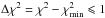 . The uncertainties of M• (ϵM) and σ (ϵσ) are considered asymmetrically in the power-law fit and the internal scatter ϵ0 is set such that the reduced χ2, i.e., the χ2 per degree of freedom, is unity after minimization. σ0 is chosen to be 200 km s-1 (as in Eq. (2)). For Eqs. (3) and (4), σ0 becomes M0 = 1011 M⊙ and L0 = 1011 M⊙, respectively. We used the IDL routine PMFITEXY1 (Williams et al. 2010) and extended it to account for asymmetric errorbars. The final values of the fit are given in Table 3, which compares the fit parameters from different methods.
3.2. Treating upper limits
The methods developed by Feigelson & Nelson (1985) and Isobe et al. (1986) combine survival analysis with astronomical applications such as determining correlation coefficients and linear regression parameters. The basic ingredients are the survival function S(zi) (the probability that the object is not detected until zi) and the hazard function λ(zi) (the instantaneous rate of detection at zi given that the object is undetected before zi). These functions are used to construct statistical quantities and also consider the non-detections.
A package of Fortran routines called ASURV2 is available for this purpose. The package contains routines for determining non-parametric correlation coefficients such as the Cox proportional hazard (CPH) model (Eq. (21) in Isobe et al. 1986), the generalized Kendall rank correlation (Eq. (28)), and linear regression methods such as the expectation-maximization (EM) algorithm with different distributions. We applied the routines to our data and list the results in Table 2 for the correlations and Table 3 for the linear regression parameters. For the generalized Kendall rank correlation the routine does not calculate τ itself but the number of standard deviations from zero (![\hbox{$z=\tau/[\rm{Var}(\tau)]^{\frac 1 2}$}](/articles/aa/full_html/2013/07/aa21183-13/aa21183-13-eq274.png) , where Var(τ) is the variance of τ under the null hypothesis). From this value, the significance of a correlation between the two variables (P) can be found from a table of the integrated Gaussian distribution. For the CPH model a χ2 value is defined to test for the significance of a correlation and the probability is taken from χ2 distribution tables.
, where Var(τ) is the variance of τ under the null hypothesis). From this value, the significance of a correlation between the two variables (P) can be found from a table of the integrated Gaussian distribution. For the CPH model a χ2 value is defined to test for the significance of a correlation and the probability is taken from χ2 distribution tables.
We stress that survival analysis a) assumes detections to be exact measurements, i.e., does not treat uncertainties and b) treats upper limits as absolute values, above (or below) where the data are definitely not detected. Since neither is the case for our data, the results have to be treated with care.
3.3. Combining uncertainties and upper limits
To treat upper limits and uncertainties in a dataset simultaneously, Kelly (2007) developed a Bayesian method that accounts for measurement errors in linear regression. This method is based on a maximum likelihood approach that is generalized to deal with multiple independent variables, nondetections (upper limits), and selection effects.
The basic approach of the routine (available as IDL routine LINMIX_ERR in the Astrolib package) is to generate a random sample of the regression parameters drawn from the probability distribution of the parameters given the measured data using a Markov chain Monte Carlo algorithm. For each iteration the regression parameters and the parameters of the prior density are updated until the Markov chain converges to the posterior distribution. The saved parameter values can then be treated as a random draw from the posterior. The final values are derived through the mean or median of the random draw.
To perform the Markov chain, two methods are available: the first one is the Gibbs sampler, which simulates new values of the model parameters and missing data at each iteration depending on the values of the observed data, current model parameters, and missing data (Kelly 2007). The second method is the Metropolis-Hastings algorithm (e.g. Metropolis et al. 1953; Hastings 1970) which is used when the selection function is not independent of the dependent variables y, the measurement errors are large, or the sample size is small. Since this is the case for our sample, we used the Metropolis-Hastings algorithm to determine the regression parameters (for more details we refer to Kelly 2007). In Table 3 we list the parameters obtained with this method. For the subsequent analysis we adopted the results of the Bayesian method as the derived fit.
Best-fit parameters for the three main scaling relations obtained form different fitting routines.
4. Discussion
In this section we discuss the results listed in Table 3 and compare the resulting correlations of IMBHs with the existing scaling relations of SMBHs in galaxies.
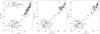 |
Fig. 2 M• − σ, M• − Mtot, and M• − Ltot relations of IMBHs and SMBHs in comparison. The slope of the best fit to the GCs (green line) is a factor of two shallower than the slope for the SMBHs in galaxies (blue line) for M• − σ, but very similar for the remaining two correlations. |
4.1. The three main scaling relations
The first correlations we studied are the ones observed in galaxies. Comparing these scaling relations with those obtained for GCs might shed light onto their origin and the evolution of GCs. Therefore, we first examined the relations M• − σ, M• − Mtot, and M• − L. We tested for the significance of a correlation by applying the methods described in the previous section. Table 2 lists the results of the Kendall τ test from standard statistics compared with the generalized Kendall τ and the results from the CPH model from survival analysis. The value P gives the probability of an existing correlation between the two values and shows high significance (>90%) for all three correlations with all methods. The highest probability is found for the M• − σ relation when using the generalized Kendall τ, but when regarding only the standard statistics, the M• − Mtot is given the highest significance. It is also the correlation with the most stable results over all three methods.
The existence of these correlations agrees with previous measurements of SMBHs in galaxies, where the same main scaling relations where found. We applied a linear regression to all three relations, using the methods described in the previous sections. In Fig. 2 we show the three scaling relations, overplotted by the best fits from the Bayesian method (green line in Fig. 1). For the M• − σ relation, all parameters of the linear regression from the different methods agree within their errorbars. The parameters derived from the different survival analysis methods are almost identical. In general, the plots show that the values of the survival analysis do not differ much from each other for all correlations. The same is true for the FITEXY method and the Bayesian approach, which shows that the errorbars have a stronger effect on the fit than the upper limits.
Comparing these values with slopes obtained for SMBHs in galaxies (Fig. 2, blue line) yields a significant difference for the slope of the correlation between galaxies and GCs in the M• − σ relation. The most recent slope obtained from McConnell & Ma (2013) is βσ = 5.64 ± 0.32, a factor of two higher than the value that we measured for the GCs. This is also visible in Fig. 2 where the values for the galaxies and the GCs are overplotted. The M• − σ relation seems to be curved upward when reaching the very high-mass black holes and becomes more shallow when reaching the low-mass range.
Moreover, for the M• − Mtot and M• − Ltot correlation all IMBH masses lie above the correlation found for galaxies but, as shown in Fig. 2, the slopes of the correlations do not differ as much as they do for the M• − σ relation. In fact, with β = 1.11 ± 0.13 for M• − Ltot and β = 1.05 ± 0.11 for M• − Ltot, the values obtained by McConnell & Ma (2013) agree with the values from Table 3 within their uncertainties.
One possible explanation for the difference in the scaling relations could be a strong mass-loss of GCs in the early stages of their evolution. Especially for ω Centauri, NGC 1851, and G1 this could have had a considerable effect because these objects were suggested to be cores of stripped dwarf galaxies (Freeman 1993; Meylan et al. 2001; Jalali et al. 2012; Sollima et al. 2012). A higher mass in the early stage of evolution of these objects would have shifted the points in all three plots to the right and therefore closer to the correlations observed for galaxies. The strongest difference in slopes is shown in the M• − σ relation. Expansion due to mass loss and relaxation would lead to an decrease of the velocity dispersion and could explain the different effect on Mtot and σ.
Another explanation would be a different mass-radius relation for galaxies and GCs which complicates the comparison of the scaling relations as the velocity dispersion is measured from an effective radius in both systems. Since GCs and galaxies are different objects, formed in different environments and processes, this explanation seems reasonable and is discussed in Graham (2013) and references therein. The fact that our relations match with the results found for nuclear star clusters (Graham 2012; Neumayer & Walcher 2012), which are found to exhibit shallow slopes, similar to GCs, supports this theory. Furthermore, clusters in our sample with upper limits still have a probability of hosting smaller IMBHs not detected up to date. This would bias all the relations toward high IMBH masses and could partly explain the difference in slopes. In fact, this is indicated by the steeper slopes from the survival analysis (where we consider only upper limits but no errorbars) as shown in Fig. 1.
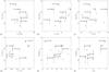 |
Fig. 3 IMBH masses as a function of several cluster properties such as a) the distance of the cluster to the sun (DSUN), b) the distance from the Galactic center (DGC), c) the metallicity ([Fe/H]), d) the ellipticity (e = 1 − b / a), e) the concentration parameter c, and f) the half-mass radius (rh). |
4.2. Are there more correlations?
The three main scaling relations discussed above are known for galaxies that host SMBHs at their centers. Even for the cases where the slopes of the IMBH correlations agree with the SMBH, it does not imply a causal connection. Formation scenarios and co-evolution of host system and black hole are assumed to be quite different for galaxies and GCs. For this reason it is crucial to search for fundamental correlations of cluster-specific values with the mass of the IMBH. This has never been done before. This section is dedicated to describe the choice of parameters and the results on their correlation significance.
4.2.1. Distances
The first parameter we checked is the distance to the sun (DSUN). No correlation is expected with this parameter, but it can be used to exclude observational biases that might be introduced to the measurements. The farther away the object, the larger one would expect the uncertainty on the black-hole mass to be. Panel a) of Fig. 3 shows the black-hole mass as a function of distance for all Galactic GCs in our sample. We excluded G1 from the plot (but not from the analysis) because it is the only cluster outside the Milky Way and its large distance would distort the figure. From the plot no evident correlation between DSUN and M• can be found, but the correlation coefficients in Table 2 show a wide spread, reaching from a slight anti-correlation for the standard Kendall τ to a significant correlation when using survival analysis. The reason for this mismatch might arise from the outlier position of G1 compared with the other distances.
As another parameter we studied the distance of the cluster to the Galactic center (in case of G1 to the center of M31), i.e., the position of the cluster in its host galaxy (DGC). Finding a correlation or anticorrelation with galactocentric distance could invite speculations about a connection between environment and black-hole formation, although the clusters are most probably not at the same distance where they were formed. Panel b) and the results in Table 2 indicate no correlation with DGC.
4.2.2. Metallicity
In Panel c) we correlate the black-hole mass with the metallicity of the cluster. A cluster with a low metallicity might be more likely to form a massive black hole through runaway merging of massive stars because of the lack of strong stellar winds at low metallicities (e.g. Vanbeveren et al. 2009). However, according to Fig. 3c and the values in Table 2, this does not seem to be the case.
4.2.3. Morphology
The lower panels in Fig. 3 depict the black-hole mass as a function of the three structural parameters: ellipticity (e), concentration (c), and half-mass radius (rh). The reason why we tested for correlations in these parameters lies in the possible connection between morphology and the cluster being the nucleus of an accreted dwarf galaxy. For example, a high ellipticity would speak against GCs, which are assumed to be spherical and dynamically relaxed systems and for a remnant of a dwarf galaxy where aspherical shapes are more common. In the same context, an IMBH in a dwarf galaxy is thought to be more massive than in a GC since more mass was available at its formation.
Furthermore, it has been shown that a black hole prevents core collapse and extends the inner regions of the cluster (e.g. Baumgardt et al. 2005). Therefore, a correlation of the central concentration with black-hole mass would be expected. Clusters with large half-mass radii have also been suggested to be good candidates of clusters hosting IMBHs at their centers. The highest correlation significance is found for the half-mass radius, but for the ellipticity a 1 − 2σ detection of correlation is present as well. For the concentration, the values of the different methods show strong variations ranging from 18% to 67%. In summary, the structural parameters and the black-hole mass show signs of correlations. However, the detection significance is low and needs to be confirmed with a larger data set.
5. Summary and conclusions
We collected data from the literature from GCs that were examined for the existence of a possible IMBH at their center using stellar dynamics. Our sample consists of 14 GCs with kinematically measured black-hole masses: six of them are thought to host IMBHs, the remaining ones have only upper limits on black-hole masses. To take uncertainties and upper limits into account, we used different methods to derive the correlation coefficients and linear regression parameters. We plotted the masses of the central IMBH versus several properties of the host clusters, such as total mass, total luminosity, and velocity dispersion to verify existing correlations that are found in galaxies, but also in the attempt to find new correlations between black-hole mass and cluster properties. We found that the three main correlations that are observed in galaxies (M• − σ, M• − Mtot, and M• − Ltot) also hold for IMBHs. The slope of the M• − σ relations differs by a factor of two from the fits made to the galaxy sample while the remaining correlations are more similar to those observed for galaxies.
Furthermore, we tested for possible correlations of the IMBH mass and other properties of the GC such as distance, metallicity, structural properties, and size. We found no evidence for a correlation as strong as the M• − σ relation, but we found a trend of black-hole mass with the cluster size, i.e., the half-mass radius rh and its ellipticity. This is reasonable since the central black hole leads the cluster to expand by accelerating stars in its vicinity.
We assume in the following that the M• − σ relation is tight, has a physical origin, and extends to the lowest masses. These assumptions have not rigorously been demonstrated to date. We also assume that the IMBHs in GCs formed at high redshifts and did not evolve much since then, unlike the GCs themselves, which will have suffered mass loss during their evolution. With these assumptions, a proposed explanation for this behavior is the process of stripping, which might have occurred to these stellar systems when accreted to the Milky Way. If they were more massive and luminous in the past, they would have fit to the correlation of the galaxies instead of being shifted to the low-mass end. These stripping scenarios have previously been suggested for clusters like G1 and ω Centauri, as mentioned in Sect. 1. In particular, because clusters most probably lost most of their mass during their lifetime and galaxies gained mass during their merging history, it would be very surprising to find both objects on the same scaling relation.
The fact that the M• − σ shows higher discrepancies when comparing the relation of galaxies than M• − Mtot and M• − Ltot might arise from either different mass-radius relations of these very different black-hole host systems or from the expansion-driven decrease of the velocity dispersion in GCs. This is supported by the fact that the scaling relations agree with the upper limits for nuclear clusters, which are stellar systems similar to GCs. N-body simulations and semi-analytic expansion models are needed to quantitatively study these theories. We note that a bias toward higher black-hole masses due to detection limits cannot be excluded either.
For the future we aim to extend this sample and confirm the reported correlations and their slopes. With integral-field units combined with adaptive optics, the search for IMBHs can be extended to extragalactic sources. Nevertheless, a complete search of Galactic GCs will provide a larger sample and help to additionally constrain critical observables that hint at the presence of an IMBH in the center of a GC.
Available at: http://purl.org/mike/mpfitexy
Available at: http://astrostatistics.psu.edu/statcodes/asurv
Acknowledgments
This research was supported by the DFG cluster of excellence Origin and Structure of the Universe (http://www.universe-cluster.de). H.B. acknowledges support from the Australian Research Council through Future Fellowship grant FT0991052. N.L. thanks Eric Feigelson, Brandon Kelly and Michael Williams for their friendly support and for providing the essential software used in this work. We thank the referee for constructive comments and suggestions that helped to improve this manuscript.
References
- Anderson, J., & van der Marel, R. P. 2010, ApJ, 710, 1032 [NASA ADS] [CrossRef] [Google Scholar]
- Bahcall, J. N., & Wolf, R. A. 1976, ApJ, 209, 214 [NASA ADS] [CrossRef] [Google Scholar]
- Barth, A. J., Ho, L. C., Rutledge, R. E., & Sargent, W. L. W. 2004, ApJ, 607, 90 [NASA ADS] [CrossRef] [Google Scholar]
- Bash, F. N., Gebhardt, K., Goss, W. M., & Van den Bout, P. A. 2008, AJ, 135, 182 [NASA ADS] [CrossRef] [Google Scholar]
- Baumgardt, H., Hut, P., Makino, J., McMillan, S., & Portegies Zwart, S. 2003, ApJ, 582, L21 [NASA ADS] [CrossRef] [Google Scholar]
- Baumgardt, H., Makino, J., & Hut, P. 2005, ApJ, 620, 238 [NASA ADS] [CrossRef] [Google Scholar]
- Colbert, E. J. M., & Mushotzky, R. F. 1999, ApJ, 519, 89 [NASA ADS] [CrossRef] [Google Scholar]
- Cseh, D., Kaaret, P., Corbel, S., et al. 2010, MNRAS, 406, 1049 [NASA ADS] [Google Scholar]
- Di Matteo, T., Springel, V., & Hernquist, L. 2005, Nature, 433, 604 [NASA ADS] [CrossRef] [PubMed] [Google Scholar]
- Dull, J. D., Cohn, H. N., Lugger, P. M., et al. 1997, ApJ, 481, 267 [NASA ADS] [CrossRef] [Google Scholar]
- Fabbiano, G. 1989, ARA&A, 27, 87 [NASA ADS] [CrossRef] [Google Scholar]
- Fabbiano, G., Zezas, A., & Murray, S. S. 2001, ApJ, 554, 1035 [NASA ADS] [CrossRef] [Google Scholar]
- Farrell, S. A., Webb, N. A., Barret, D., Godet, O., & Rodrigues, J. M. 2009, Nature, 460, 73 [NASA ADS] [CrossRef] [PubMed] [Google Scholar]
- Feigelson, E. D., & Nelson, P. I. 1985, ApJ, 293, 192 [NASA ADS] [CrossRef] [Google Scholar]
- Feldmeier, A., Lützgendorf, N., Neumayer, N., et al. 2013, A&A, 554, A63 [NASA ADS] [CrossRef] [EDP Sciences] [Google Scholar]
- Ferrarese, L., & Ford, H. 2005, Space Sci. Rev., 116, 523 [NASA ADS] [CrossRef] [Google Scholar]
- Ferrarese, L., & Merritt, D. 2000, ApJ, 539, L9 [NASA ADS] [CrossRef] [Google Scholar]
- Filippenko, A. V., & Ho, L. C. 2003, ApJ, 588, L13 [NASA ADS] [CrossRef] [Google Scholar]
- Freeman, K. C. 1993, in The Globular Cluster-Galaxy Connection, ASP Conf. Ser., 48, 608 [Google Scholar]
- Gebhardt, K., Pryor, C., Williams, T. B., Hesser, J. E., & Stetson, P. B. 1997, AJ, 113, 1026 [NASA ADS] [CrossRef] [Google Scholar]
- Gebhardt, K., Bender, R., Bower, G., et al. 2000a, ApJ, 539, L13 [NASA ADS] [CrossRef] [Google Scholar]
- Gebhardt, K., Pryor, C., O’Connell, R. D., Williams, T. B., & Hesser, J. E. 2000b, AJ, 119, 1268 [NASA ADS] [CrossRef] [Google Scholar]
- Gebhardt, K., Rich, R. M., & Ho, L. C. 2002, ApJ, 578, L41 [NASA ADS] [CrossRef] [Google Scholar]
- Gebhardt, K., Rich, R. M., & Ho, L. C. 2005, ApJ, 634, 1093 [NASA ADS] [CrossRef] [Google Scholar]
- Gebhardt, K., Adams, J., Richstone, D., et al. 2011, ApJ, 729, 119 [NASA ADS] [CrossRef] [Google Scholar]
- Gerssen, J., van der Marel, R. P., Gebhardt, K., et al. 2002, AJ, 124, 3270 [NASA ADS] [CrossRef] [Google Scholar]
- Godet, O., Barret, D., Webb, N. A., Farrell, S. A., & Gehrels, N. 2009, ApJ, 705, L109 [NASA ADS] [CrossRef] [Google Scholar]
- Graham, A. W. 2012, MNRAS, 422, 1586 [NASA ADS] [CrossRef] [Google Scholar]
- Graham, A. W. 2013, Planets, Stars and Stellar Systems (Berlin: Springer), 6, 91 [CrossRef] [Google Scholar]
- Gültekin, K., Richstone, D. O., Gebhardt, K., et al. 2009, ApJ, 698, 198 [NASA ADS] [CrossRef] [Google Scholar]
- Häring, N., & Rix, H. 2004, ApJ, 604, L89 [NASA ADS] [CrossRef] [Google Scholar]
- Harris, W. E. 1996, AJ, 112, 1487 [NASA ADS] [CrossRef] [Google Scholar]
- Hastings, W. 1970, Biometrika, 57, 97 [Google Scholar]
- Hlavacek-Larrondo, J., Fabian, A. C., Edge, A. C., & Hogan, M. T. 2012, MNRAS, 424, 224 [NASA ADS] [CrossRef] [Google Scholar]
- Hopkins, P. F., Hernquist, L., Cox, T. J., Robertson, B., & Krause, E. 2007, ApJ, 669, 45 [NASA ADS] [CrossRef] [Google Scholar]
- Ibata, R., Bellazzini, M., Chapman, S. C., et al. 2009, ApJ, 699, L169 [NASA ADS] [CrossRef] [Google Scholar]
- Isobe, T., Feigelson, E. D., & Nelson, P. I. 1986, ApJ, 306, 490 [NASA ADS] [CrossRef] [Google Scholar]
- Jalali, B., Baumgardt, H., Kissler-Patig, M., et al. 2012, A&A, 538, A19 [NASA ADS] [CrossRef] [EDP Sciences] [Google Scholar]
- Kelly, B. C. 2007, ApJ, 665, 1489 [NASA ADS] [CrossRef] [Google Scholar]
- Kong, A. K. H. 2007, ApJ, 661, 875 [NASA ADS] [CrossRef] [Google Scholar]
- Kormendy, J., & Richstone, D. 1995, ARA&A, 33, 581 [NASA ADS] [CrossRef] [Google Scholar]
- Lützgendorf, N., Kissler-Patig, M., Noyola, E., et al. 2011, A&A, 533, A36 [NASA ADS] [CrossRef] [EDP Sciences] [Google Scholar]
- Lützgendorf, N., Kissler-Patig, M., Gebhardt, K., et al. 2012, A&A, 542, A129 [NASA ADS] [CrossRef] [EDP Sciences] [Google Scholar]
- Lützgendorf, N., Kissler-Patig, M., Gebhardt, K., et al. 2013, A&A, 552, A49 [NASA ADS] [CrossRef] [EDP Sciences] [Google Scholar]
- Ma, J., de Grijs, R., Chen, D., et al. 2007, MNRAS, 376, 1621 [NASA ADS] [CrossRef] [Google Scholar]
- Maccarone, T. J., & Servillat, M. 2008, MNRAS, 389, 379 [NASA ADS] [CrossRef] [Google Scholar]
- Maccarone, T. J., Fender, R. P., & Tzioumis, A. K. 2005, MNRAS, 356, L17 [NASA ADS] [Google Scholar]
- Marconi, A., & Hunt, L. K. 2003, ApJ, 589, L21 [NASA ADS] [CrossRef] [Google Scholar]
- Matsumoto, H., Tsuru, T. G., Koyama, K., et al. 2001, ApJ, 547, L25 [NASA ADS] [CrossRef] [Google Scholar]
- McConnell, N. J., & Ma, C.-P. 2013, ApJ, 764, 184 [NASA ADS] [CrossRef] [Google Scholar]
- McConnell, N. J., Ma, C.-P., Gebhardt, K., et al. 2011, Nature, 480, 215 [NASA ADS] [CrossRef] [Google Scholar]
- McLaughlin, D. E., & van der Marel, R. P. 2005, ApJS, 161, 304 [NASA ADS] [CrossRef] [Google Scholar]
- McLaughlin, D. E., Anderson, J., Meylan, G., et al. 2006, ApJS, 166, 249 [NASA ADS] [CrossRef] [Google Scholar]
- Metropolis, N., Rosenbluth, A. W., Rosenbluth, M. N., Teller, A. H., & Teller, E. 1953, J. Chem. Phys., 21, 1087 [NASA ADS] [CrossRef] [Google Scholar]
- Meylan, G., Mayor, M., Duquennoy, A., & Dubath, P. 1995, A&A, 303, 761 [NASA ADS] [Google Scholar]
- Meylan, G., Sarajedini, A., Jablonka, P., et al. 2001, AJ, 122, 830 [NASA ADS] [CrossRef] [Google Scholar]
- Miller, M. C., & Hamilton, D. P. 2002, MNRAS, 330, 232 [NASA ADS] [CrossRef] [MathSciNet] [Google Scholar]
- Miller-Jones, J. C. A., Wrobel, J. M., Sivakoff, G. R., et al. 2012, ApJ, 755, L1 [NASA ADS] [CrossRef] [Google Scholar]
- Neumayer, N., & Walcher, C. J. 2012, Adv. Astron., 2012 [Google Scholar]
- Noyola, E., & Baumgardt, H. 2011, ApJ, 743, 52 [NASA ADS] [CrossRef] [Google Scholar]
- Noyola, E., Gebhardt, K., & Bergmann, M. 2008, ApJ, 676, 1008 [NASA ADS] [CrossRef] [Google Scholar]
- Noyola, E., Gebhardt, K., Kissler-Patig, M., et al. 2010, ApJ, 719, L60 [NASA ADS] [CrossRef] [Google Scholar]
- Pasquini, L., Avila, G., Blecha, A., et al. 2002, The Messenger, 110, 1 [NASA ADS] [Google Scholar]
- Peterson, R. C., Seitzer, P., & Cudworth, K. M. 1989, ApJ, 347, 251 [NASA ADS] [CrossRef] [Google Scholar]
- Pooley, D., & Rappaport, S. 2006, ApJ, 644, L45 [NASA ADS] [CrossRef] [Google Scholar]
- Silk, J., & Arons, J. 1975, ApJ, 200, L131 [NASA ADS] [CrossRef] [Google Scholar]
- Silk, J., & Rees, M. J. 1998, A&A, 331, L1 [NASA ADS] [Google Scholar]
- Sollima, A., Gratton, R. G., Carballo-Bello, J. A., et al. 2012, MNRAS, 426, 1137 [NASA ADS] [CrossRef] [Google Scholar]
- Soria, R., Hau, G. K. T., Graham, A. W., et al. 2010, MNRAS, 405, 870 [NASA ADS] [Google Scholar]
- Soria, R., Hau, G. K. T., & Pakull, M. W. 2013, ApJ, 768, L22 [NASA ADS] [CrossRef] [Google Scholar]
- Springel, V., Di Matteo, T., & Hernquist, L. 2005, MNRAS, 361, 776 [NASA ADS] [CrossRef] [Google Scholar]
- Stephens, A. W., Frogel, J. A., Freedman, W., et al. 2001, AJ, 121, 2597 [NASA ADS] [CrossRef] [Google Scholar]
- Strader, J., Chomiuk, L., Maccarone, T. J., et al. 2012, ApJ, 750, L27 [NASA ADS] [CrossRef] [Google Scholar]
- Tremaine, S., Gebhardt, K., Bender, R., et al. 2002, ApJ, 574, 740 [NASA ADS] [CrossRef] [Google Scholar]
- Ulvestad, J. S., Greene, J. E., & Ho, L. C. 2007, ApJ, 661, L151 [NASA ADS] [CrossRef] [Google Scholar]
- van den Bosch, R., de Zeeuw, T., Gebhardt, K., Noyola, E., & van de Ven, G. 2006, ApJ, 641, 852 [NASA ADS] [CrossRef] [Google Scholar]
- van den Bosch, R. C. E., Gebhardt, K., Gültekin, K., et al. 2012, Nature, 491, 729 [NASA ADS] [CrossRef] [PubMed] [Google Scholar]
- Vanbeveren, D., Belkus, H., van Bever, J., & Mennekens, N. 2009, Ap&SS, 324, 271 [NASA ADS] [CrossRef] [Google Scholar]
- Williams, M. J., Bureau, M., & Cappellari, M. 2010, MNRAS, 409, 1330 [NASA ADS] [CrossRef] [Google Scholar]
- Xiao, T., Barth, A. J., Greene, J. E., et al. 2011, ApJ, 739, 28 [NASA ADS] [CrossRef] [Google Scholar]
All Tables
Best-fit parameters for the three main scaling relations obtained form different fitting routines.
All Figures
|
Fig. 1 M• − σ (left), M• − MTOT (middle) and M• − LTOT (right) relation for GCs with IMBHs. The gray arrows indicate upper limits. We compare the slopes of the best-fits from four different methods. |
| In the text | |
|
Fig. 2 M• − σ, M• − Mtot, and M• − Ltot relations of IMBHs and SMBHs in comparison. The slope of the best fit to the GCs (green line) is a factor of two shallower than the slope for the SMBHs in galaxies (blue line) for M• − σ, but very similar for the remaining two correlations. |
| In the text | |
|
Fig. 3 IMBH masses as a function of several cluster properties such as a) the distance of the cluster to the sun (DSUN), b) the distance from the Galactic center (DGC), c) the metallicity ([Fe/H]), d) the ellipticity (e = 1 − b / a), e) the concentration parameter c, and f) the half-mass radius (rh). |
| In the text | |
Current usage metrics show cumulative count of Article Views (full-text article views including HTML views, PDF and ePub downloads, according to the available data) and Abstracts Views on Vision4Press platform.
Data correspond to usage on the plateform after 2015. The current usage metrics is available 48-96 hours after online publication and is updated daily on week days.
Initial download of the metrics may take a while.