© ESO, 2013

1. Introduction

The centrifugal force of rapid rotators induces a strong deformation of the stellar geometry that has been nicely shown observationally, thanks to long-baseline optical interferometrers that today allow observations at high spatial resolution to be performed (van Belle et al. 2001, 2006; Domiciano de Souza et al. 2003; McAlister et al. 2005; Kervella & Domiciano de Souza 2006; Monnier et al. 2007; Zhao et al. 2009). Concomitant to the stellar flattening, there is a non-uniform effective temperature distribution, called the gravity darkening effect (GDE; von Zeipel 1924). For stars with conservative rotation laws (rigid rotation is a particular case of a conservative law), whose envelopes are in hydrostatic and radiative equilibrium and where the diffusion approximation to the radiative transfer equation is used, the following relation for the effective temperature distribution as a function of the co-latitude θ holds: ${\mathit{T}}_{\mathrm{eff}}\mathrm{\left(}\mathit{\theta }\mathrm{\right)}\mathrm{=}{\mathit{T}}_{\mathrm{p}}{\left[\frac{{\mathit{g}}_{\mathrm{eff}}\mathrm{\left(}\mathit{\theta }\mathrm{\right)}}{{\mathit{g}}_{\mathrm{p}}}\right]}^{\mathit{\beta }}\mathit{,}$(1) where T_eff(θ) and g_eff(θ) are the co-latitude θ dependent effective temperature and effective gravity T_p is the polar effective temperature, and g_p is the polar gravity. The canonical value β = 0.25 (i.e., the standard gravity-darkening law von Zeipel 1924) is thus valid only in the frame of the above-mentioned physical conditions and approximations. The value β = 0.08 holds for stars with convective envelopes (Lucy 1967; Reiners 2003). Tuominen (1972) also found that β = 0.15 for non-barotropic differentially rotating stars with masses M ≃ 2.5 M_⊙. In a recent work, Zorec et al. (2011, and references therein) commented that β < 0.25 may reveal a non-conservative rotational law in the stellar surface. Nevertheless, when more detailed expressions for the radiative flux are used and not simply the diffusion approximation, β ≲ 0.25 (Claret 2012). Che et al. (2011) suggested β = 0.19 for rapid rotators, and Espinosa Lara & Rieutord (2012) showed that β ranges from 0.25 for slow rotators and decreases for rapid rotators, compatible with observations of Che et al. (2011).

Rotation generates hydrodynamical instabilities that redistribute the angular momentum in the stellar interior. Some of them were taken into account to study their effect on the stellar structure and evolution with rotation (cf. Endal & Sofia 1979; Pinsonneault et al. 1991; Heger & Langer 2000; Meynet & Maeder 2000). These instabilities also induce a turbulent diffusion (Zahn 1992) that, in massive objects, distributes the CNO-cycled material from the core to the envelope and changes the stellar atmospheric chemical composition profile (Meynet & Maeder 2000). Owing to the mass-compensation effect related to the rapid rotation (Sackmann 1970), the total radiative flux produced in the stellar core is lower than that of a parent rotationless star. The combined effect of the mass-compensation effect and the refueling of the stellar core by the meridian circulation contributes to extend the lifespan of stars in the main sequence (cf. Kiziloglu & Civelek 1996; Talon et al. 1997; Meynet & Maeder 2000). Stellar winds and the related continuum mass-loss rate are somewhat modified by the rotation (Lamers & Cassinelli 1999; Maeder et al. 2007). Maeder et al. (2008) have shown that in massive stars, rapid rotation considerably enlarges the Fe and He ionization-related convective zones in their envelope. This convection can then induce a non-conservative, albeit non-shellular, law of differential rotation in the envelope, on which rely both the stellar external geometry and its surface brightness distribution (Zorec et al. 2011).

This account of observational phenomena related with rotation shows that all stellar observables, in particular those we can obtain with interferometry, can be complex functions of several fundamental parameters, some of intrinsic stellar nature (mass, age, chemical composition, amount of angular momentum stored in the star, rotation law, etc.) and others of more geometrical or extrinsic character (inclination angle, position in the sky, etc.). The stellar geometry and the wavelength-dependent surface brightness distribution are both measurable with interferometric techniques. We can then ask whether by using observables, some of the quoted independent parameters can be tested individually, or whether they should all be determined and analyzed at once.

At a first glance, we may expect that due to their extrinsic nature, the position angle of the rotation axis and the stellar inclination can be determined independently of the stellar parameters of intrinsic character, even though the determination of the inclination angle relies on the surface brightness asymmetries, which in turn are controlled by intrinsic stellar quantities.

The aim of the present paper is the following: thanks to a spectral resolution that can reach 30 000, the VEGA/CHARA instrument (Mourard et al. 2009, 2010) offers a great possibility to perform precise measurements of differential phases of fringes to study the prevailing kinematics in the stellar atmospheres. By taking advantage of the link that exists between the phase of fringes and the position of the photo-center in a partially resolved star, we can carry out spectro-interferometric studies and provide measurements of the position angle (PA) of stars. A similar approach was recently used to measure the PA of the rotation axis of the fast rotators Fomalhaut (Le Bouquin et al. 2009) and Achernar (Domiciano de Souza et al. 2012a). In addition, this work differs from previous studies of the PA (van Belle et al. 2006; Zhao et al. 2009), because we use information on the stellar atmosphere from the observed spectral lines. The method is tested for α Cep using the Hα absorption line.

In principle, the combination of the high spectral and spatial resolution should enable us to extract information from the surface radial iso-velocity curves, whose properties reflect the kinematics in the stellar atmosphere. The apparent aspect of the radial iso-velocity curves depends, however, on the inclination angle i of the rotation axis, and on the degree of the surface differential rotation. It is then worthwhile to discuss whether we can estimate the inclination angle i and the degree of differential rotation independently of the intrinsic stellar parameters.

The present paper is organized as follows: in Sect. 2 we summarize previous studies of α Cep. In Sect. 3, we present our interferometric observations and reduction technique. In Sect. 4, we introduce our method for deriving the position angle PA of the stellar rotation axis. In this section, we also introduce the model used to interpret the interferometric measurements and present the results obtained with our best model. In Sect. 5 we study the effects on the von Zeipel coefficient β determination that depend on the law of surface differential rotation and analyze the feasibility of the inclination angle i determination. The conclusions are summarized in Sect. 6.

2. α Cephei

α Cephei (Alderamin, HD 203 280, HR 8162, V = 2.46, d = 14 pc) is the brightest star in the constellation of Cepheus. Originally classified as A2n (Douglas 1926), the spectral type of α Cephei has been re-estimated in Johnson & Morgan (1953), who classified it as A7IV-V. Gray et al. (2003) classified the star as A8V. Like Altair, α Cep has a chromosphere (Walter et al. 1995; Simon & Landsman 1997; Simon et al. 2002). According to various authors, the Vsini of α Cep ranges from 180 km s^-1 to 245 km s^-1 (Bernacca & Perinotto 1973a,b,c; Uesugi & Fukuda 1970; Royer et al. 2007; Abt & Morrell 1995).

Up to now, few interferometric observations have been carried out on α Cep. van Belle et al. (2006) used the Georgia State University CHARA array to observe this star in the infrared and estimated its oblateness, the rotational velocity, and its gravity darkening. Their data showed a non-circular projected disk brightness distribution from which they deduced the equatorial and polar diameter of α Cep using two different models. The first one, purely geometrical, represents an elliptical star whose brightness distribution is uniform. From this model, they found a polar diameter of 1.355 ± 0.080 mas, an equatorial diameter of 1.625 ± 0.056 mas and a position angle of the rotation axis of 3° ± 14° (or −177°, since there can be an indetermination of 180°) with a reduced χ² of 1.08. The second, and more physical model, takes into account the shape of the photosphere under conditions of hydrostatic equilibrium, uniform rotation, Roche’s approximation for the total potential at the surface, the limb darkening that responds to the geometrical deformation of the star, and the surface gravity darkening. The parameters derived from their best model are summarized in Table 1. Their estimate of the β exponent in the gravitational darkening law gives $\mathit{\beta }\mathrm{=}\mathrm{0.08}{\mathrm{4}}_{-0.049}^{\mathrm{+}\mathrm{0.026}}$, which is consistent with β = 0.08 expected for a star whose envelope is entirely convective (Lucy 1967; Reiners 2003).

Taking advantage of a better (u,v)-plane coverage than in van Belle et al. (2006), Zhao et al. (2009) used the Michigan Infra-Red Combiner (MIRC) at the CHARA Array to produce a model for α Cep as fast rotator. These authors calculated models of brightness distribution in fast rotating stars according to prescriptions given by Aufdenberg et al. (2006, and references therein), which they fitted to the interferometric observations. In these models the authors assumed solid-body rotation, adopted a Roche potential to characterize the stellar surface, and used the von Zeipel gravity darkening law (von Zeipel 1924) to determine the latitude-dependent effective temperature profile. Hence, for α Cep they deduced the inclination angle i, the position angle PA of the rotation axis, the polar R_pol and equatorial R_eq radii, the polar effective temperature T_p, and equatorial effective temperature T_eq, the angular velocity ratio ω = Ω/Ω_c, and the β exponent. These values are summarized in Table 1.

The exponent β = 0.216 ± 0.021 found by Zhao et al. (2009) suggests that the envelope of α Cep is probably not convective as found by van Belle et al. (2006). Because their β exponent is lower than 0.25, at least three possibilities exist: 1) the stellar envelope is mostly radiative but interspersed with convective regions, which in the equatorial region case perhaps induced by the GDE where the effective temperature is low enough; 2) the surface rotation reflects a deeper non-conservative rotation law in the envelope; or 3) the diffusion approximation used to derive the gravity darkening law is not sufficient, and more detailed expressions for the emerging radiative flux must be taken into account (Claret 2012).

3. Observations and data reduction

3.1. Observations

The VEGA instrument (Mourard et al. 2009) at the CHARA Array (ten Brummelaar et al. 2005), located on the Mount Wilson Observatory (LA, California, USA), operates in the visible domain and benefits from a spectrograph and a polarimeter. The spectrograph is designed to sample in the visible band from 0.45 to 0.85 μm and is equipped with two photon-counting detectors that observe in two different spectral bands (the detector that observes at the shortest wavelength is denoted “blue”, the other is called “red”). Interferometric observations of α Cep with the VEGA/CHARA instrument were carried out in July 2008 and October 2010 using the high spectral resolution mode (R = 30 000). All observations were made with two telescopes only. Observations were conducted with the red and blue detectors centered at 656 nm (Hα line) and 632 nm, respectively. In this spectral resolution mode, the Hα line covers almost the entire surface of the red detector, which allows us to make a precise measurement of the differential phase. Because we based our study on a differential analysis, we did not need to observe calibrators. The log of the observations is given in Table 2 and the (u,v)-plane coverage during these observation campaigns is shown in Fig. 1.

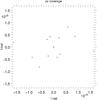Fig. 1 (u,v)-plane coverage by our observations (u is in abscissas).

3.2. Data reduction

The data were reduced with the software developed in the VEGA group and described by Mourard et al. (2009). This software offers two data reduction modes, the first one is the spectral density analysis and the second one the cross-spectral analysis scheme. In the spectral density mode, we only obtain the squared visibility averaged over a spectral band centered at a given wavelength λ₁. With the cross-spectral analysis mode, we obtain a visibility modulus V(λ) and a differential phase φ_diff within a narrow channel of a few angstroms, which is step-by-step translated over a large reference spectral band. In each step, we measure the product V(λ₁) × V(λ₂) and φ_diff(λ₁). In this study, we are only interested by the quantity φ_diff(λ₁). The spectral calibration was performed with known spectral lines of the ThAr spectral lamp. A polynomial fit was made to determine the dispersion law. The residual of the fit is typically two times lower than the spectral resolution.

Figure 2 presents the differential phases obtained after the data processing. In this figure we also superimposed (red solid line) the best-fit model. As explained in Sect. 4.4, the differential phases in the wings of the H_α line (outside 6555 Å to 6569 Å) can be considered to be equal to zero. We used the measurements in this “wings” region to estimate the variance of the phase and decided to attribute this variance to the individual phase error. We then applied a fit of the model in the S-shaped region, where a signal is expected, i.e. from 6555 Å to 6569 Å.

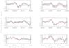Fig. 2 Differential phases obtained after data processing. This figure also shows the best-fit (red line) models calculated as a function of the position angle of the rotation axis ($\mathrm{PA}\mathrm{=}\mathrm{-}\mathrm{15}{\mathrm{7}}_{\mathrm{-}\mathrm{10}°}^{\mathrm{+}\mathrm{17}°}$) obtained as explained in Sect. 4.4.

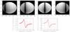Fig. 3 Top: intensity maps calculated for selected wavelengths inside the Hα line (from left to right): 6559.5 Å, 6561.3 Å, 6562.8 Å, and 6565.2 Å. Ordinates and abscissas are given in units of the equatorial radius Req. The inclination angle used is i = 55°. Bottom: photo-center displacements along the y-axis (left side); differential phase associated with the photo-center shift (right side). All quantities are computed for a sixty-meter baseline parallel to the equatorial axis (x-axis). The photo-center displacements are given in units of the angular stellar radius.

4. Determination of the position angle

4.1. Principles

Interferometric observables were modeled from a computed brightness distribution (see Sect. 4.2) using the Zernike-van Cittert’s theorem. This theorem relates the complex visibility V_δλ with a stellar surface brightness distribution emitted in a given spectral channel of bandwidth δλ: $V_{\mathit{\delta \lambda }}\mathrm{\left(}\mathit{u,v}\mathrm{\right)}\mathrm{=}\frac{{\mathrm{\int }}_{\mathrm{-}\mathrm{\infty }}^{\mathrm{\infty }}{\mathrm{\int }}_{\mathrm{-}\mathrm{\infty }}^{\mathrm{\infty }}{\mathit{I}}_{\mathit{\delta \lambda }}\mathrm{\left(}\mathit{\alpha ,\beta }\mathrm{\right)}\exp \mathrm{[}\mathrm{-}\mathrm{2}\mathit{\pi i}\mathrm{(}\mathit{\alpha u}\mathrm{+}\mathit{\beta u}\mathrm{\left)}\mathrm{\right]}\mathrm{d}\mathit{\alpha }\mathrm{d}\mathit{\beta }}{{\mathrm{\int }}_{\mathrm{-}\mathrm{\infty }}^{\mathrm{\infty }}{\mathrm{\int }}_{\mathrm{-}\mathrm{\infty }}^{\mathrm{\infty }}{\mathit{I}}_{\mathit{\delta \lambda }}\mathrm{\left(}\mathit{\alpha ,\beta }\mathrm{\right)}\mathrm{d}\mathit{\alpha }\mathrm{d}\mathit{\beta }}\mathit{,}$(2)where I_δλ(α,β) is the intensity of the emitted energy by the source toward the observer caught in the spectral channel of bandwidth δλ and centered on the wavelength λ; (α,β) are the angular coordinates of an emitting point in the source projected onto the sky, while (u,v) are the Fourier conjugate spatial frequencies related to the baseline coordinates and measured in the observing plane. The modulus of the complex visibility, V_δλ = |V_δλ(u,v) |, measures the contrast of the interferometric fringes, while its argument determines the phase of the fringes, φ_δλ = arg [V_δλ(u,v)]. For an unresolved source, φ_δλ is directly related to the position of the photo-center of the brightness distribution at a given wavelength λ. Unfortunately, the atmospheric turbulence disrupts the phase of fringes when interferometric observations are performed with only two telescopes. To overcome this difficulty, we used the differential phase φ_diff, defined as the difference between the phase measured in two spectral channels centered on the wavelengths λ₁ and λ₂: ${\mathit{\phi }}_{\mathrm{diff}}\mathrm{=}{\mathit{\phi }}_{{\mathit{\lambda }}_{\mathrm{2}}}\mathrm{-}{\mathit{\phi }}_{{\mathit{\lambda }}_{\mathrm{1}}}\mathit{.}$(3)The quantity φ_diff enables us to quantify the displacement of photo-centers at different wavelengths λ of an unresolved source free from perturbations from the atmospheric turbulence. The spatial resolution reached with the S1S2 and E1E2 baselines used in this study are 5.5 and 2.7 mas, respectiveley, at 0.656 μm. Hence, α Cep remained unresolved (see Table 1). The cross-spectrum method described in Berio et al. (1999) and Tatulli et al. (2007) used in the VEGA/CHARA data processing aims at measuring the differential phases φ_diff(λ) and the differential visibility V_diff(λ) between two different spectral channels centered on the wavelengths λ₁ and λ₂.

4.2. Models of stellar surface brightness distribution

To calculate φ_diff and V_diff(λ) we used the model described in Domiciano de Souza et al. (2002) and Domiciano de Souza et al. (2012b), which can produce the intensity maps in the Hα line needed in this work. This model is based on the following assumptions: a) stars have rigid rotation; b) Roche-approximation is used to describe the stellar shape modified by the rigid rotation; c) at each point of the observed stellar hemisphere, the atmosphere is approximated by a plane-parallel model for the local effective temperature T_eff(θ) and gravity g(θ).

A modified version of the BRUCE/KYLIE calculation code (Townsend 1997) was used to divide the apparent hemisphere into elementary surface elements (blocks), each characterized by a given set of local physical parameters. The plane-parallel stellar atmosphere models were computed using the Kurucz stellar atmosphere models with solar abundances (Kurucz 1979). The SYNSPEC code (Hubeny & Lanz 1995) with chemical compositions compatible with metallicity Z = 0.02 was employed to calculate the local emergent specific radiation intensities directed toward the observer I_δλ(α,β) which determine the monochromatic intensity maps of the apparent photosphere in the wavelengths of the instrumental transmitting channels. The models depend on five intrinsic stellar parameters: polar radius R_p, the polar temperature T_p, the polar gravity g_p, the stellar rotational flattening D = R_e/R_p, and the gravity darkening exponent β. In addition, there are two extrinsic parameters: the stellar inclination angle i and the position angle PA of the stellar rotation axis.

4.3. Method

We adopted a Cartesian reference system in the sky centered on the star, so that the x −axis lies along the equator of the star and the y-axis contains the plane of the stellar rotation axis. In the upper panel of Fig. 3, we show the computed displacement of the photo-center of the H_α line as observed along the equatorial axis of α Cep. The corresponding differential phases φ_diff(λ) are shown in the lower panel of Fig. 3. Phases are calculated for a sixty-meter baseline parallel to the direction of the stellar equatorial axis. When the orientation of the baseline projected onto the sky changes with respect to the x-axis, we obtain different plots of φ_diff(λ), as illustrated in Fig. 4, where the line-styles change according to the orientation of the baseline. φ_diff(λ) is well spread for a baseline perpendicular to the rotational axis of the star (Mourard 1990), whereas for a baseline parallel to the rotational axis of the star, φ_diff(λ) is close to zero. So, to determine the position angle PA of the stellar rotation axis of α Cep, we carried out spectro-interferometric observations at different orientations of the baseline and took measurements of the respective variation of phases φ_diff(λ). Thus, for a given observed distribution φ_diff(λ) as a function of λ, we can estimate the PA by searching the best fit of the observed differential phases with calculated ones for different position angles.

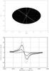Fig. 4 Differential phases φdiff(λ) in the Hα line for different baseline orientations. Top: stellar disk deformed by the fast rotation and projected onto the sky where we have represented the baseline orientations: 0° (cross), 45° (star), 90° (solid line) and 160° (diamond). Bottom: evolution of φdiff(λ) according to the baseline orientations represented on top and computed for a sixty meter-baseline. In this example we assumed that the position angle of the stellar rotation axis is equal to zero.

4.4. Model fitting

The position angle PA of the rotation axis is an extrinsic parameter whose determination can be assumed independent of the choice of the intrinsic stellar parameters. The results obtained will justify this assumption a posteriori. So, to calculate the brightness distribution, we adopted the stellar quantities R_p, T_p, g_p, D, and i obtained by Zhao et al. (2009, see Table 1) because of their excellent (u,v)-plane coverage. Then, we calculated monochromatic intensity maps for wavelengths inside the Hα line as detailed in Sect. 4.2, and for a series of angle PA and β parameters. The corresponding differential phases φ_diff(λ) were estimated by calculating the FT of the monochromatic intensity maps.

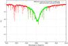Fig. 5 Spectrum of alpha Cep obtained in the high spectral resolution mode of VEGA/CHARA (green) and ith the ELODIE spectrograph (red).

It is important to note that in the high spectral resolution mode, the red detector of the VEGA/CHARA instrument covers only the spectral interval λλ6542.49−6582.68 Å of the observed H_α line of α Cep, as shown in Fig. 5. Because of the lack of measurements in the continuum spectrum around the line, we calibrated the differential phases by assuming that both line wings in the uncovered spectral ranges are symmetric. To test this hypothesis, we computed images of the apparent stellar hemisphere and the respective differential phases at four different wavelengths: λ 6548.7, 6557.7, 6562.8, and 6568.5 Å. A perfectly symmetric distribution of the stellar brightness in the given wavelengths should lead the corresponding photo-centers to lie in the center of the disk and the respective differential phases to be zero. The images of the brightness distribution over the stellar disk at the chosen wavelength are shown in Fig. 6. The values of the differential phase for each image are summarized Table 3. Because the expected uncertainty on the estimate of differential phases is roughly 3°, we conclude that in the wavelength-intervals λλ6542.49−6557.7 Å and λλ6568.5−6582.68 Å our hypothesis of wing-symmetry is a reasonable first approximation.

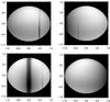Fig. 6 Surface brightness distribution in α Cep at four different wavelengths: 6548.7 Å (top, left), 6557.7 Å (top, right), λ6562.8 Å (bottom, left), and λ6568.5 Å, (bottom, right). Ordinates and abscissas are given in units of the equatorial radius Req. The inclination angle used is i = 55°.

According to the results shown in Table 3, we can assume that the differential phase in the wings of the Hα line is equal to zero, because we were dealing with the continuum spectrum proper. The differential phases in these spectral ranges were fitted with a polynomial and then used to divide the observed differential phases to obtain the sought calibration.

To determine PA, a grid of models parameterized according to the exponent β, and the position angle of the rotation axis of α Cep was produced. The β exponents used range from 0.08 to 0.25 by steps of 0.01, while the angle PA ranged from −130° to −180° by steps of 1°. This interval of PA was chosen according to previous indications on the PA value inferred in van Belle et al. (2006) and Zhao et al. (2009). Each model provides thus the observable φ_diff(λ), which is compared to the data and the fit controlled through a χ² test. In Fig. 2 are shown the respective best fits obtained (red lines) to the observed differential phases. We computed the reduced χ² residuals (hereafter χ_red) and plotted as a function of the PA angle, as shown in Fig. 7, where each curve corresponds to a different gravity darkening exponent. We note that the χ_red curves are calculated for λ6560 Å and each of them is an average over the six better fits obtained from the respective observed differential phases.

From the χ_red curves in Fig. 7 we can see that if the PA determination corresponds to the minimum value [χ²(β)_red] _min, roughly the same angle PA will be obtained whatever the β exponent. Because each β value produces a different effective temperature contrast over the observed stellar hemisphere, with the consequent contrast of the emitted radiative fluxes, which mimic the effect of different sets of intrinsic stellar parameters, we conclude that the observed differential phases φ_diff(λ) against the position angle reflect the external stellar geometry quite independently of any explicit intrinsic physical parameter.

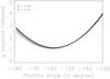Fig. 7 ${\mathit{\chi }}_{\mathrm{red}}^{\mathrm{2}}$ as a function of the PA of the rotation axis of α Cep for different von Zeipel exponents ranging from β = 0.08 to β = 0.25.

To avoid inconveniences introduced by possible correlations among data points, a reliable approach to the uncertainty affecting the estimate of the position angle PA can be inferred by using the random re-sampling of data or “bootstrap simulation” (Efron & Tibshirani 1986). We thus randomly re-sampled B = 700 times the six data sets of differential phases shown in Fig. 8 in the wavelength interval used to fit the model-differential phases. This leads to B independent determinations of PA values shown in Fig. 8a against the bootstrap replication number. The position angles of Fig. 8a were calculated for the von Zeipel coefficient β = 0.19 that was suggested in Che et al. (2011) to analyze interferometric data. The position angles PA were then gathered into a histogram of frequencies where the class-step (bin-width) ΔPA = 2° was chosen following the bin-width optimization method in Shimazaki & Shinomoto (2007). The histogram is shown in Fig. 8b, where we also show a smoothed version of the histogram obtained using the Gaussian-kernel-estimator method (Bowman & Azzalini 1997) (dashed curve). We can readily see that the estimate of PA with the highest probability is PA = −157°, while more than 99% of estimates are in the interval from PA = −167° to PA = −140° ($\mathrm{PA}\mathrm{=}\mathrm{-}\mathrm{15}{\mathrm{7}}_{\mathrm{-}\mathrm{10}°}^{\mathrm{+}\mathrm{17}°}$). The whole fitting procedure was also repeated for β = 0.08 and β = 0.25. While the confidence interval remains in all cases the same, for β = 0.08 the maximum is slightly shifted to more negative values of PA and slightly to more positive PA for β = 0.25 than with β = 0.19, but the whole displacement implies ΔPA ≃ 2°. The low value of Δβ demonstrates the high independence of the PA-angle determination on the chosen value of β.

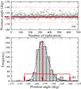Fig. 8 a) Simulated position angle PA against the number of “bootstrap” replications when β = 0.19. The colored line indicates the position angle PA of maximum probability. b) Frequency distribution of the simulated position angles PA (histogram and smoothed distribution). In the figure are also indicated the position angle PA of maximum probability and the 99% confidence interval.

The contrast of the brightness distribution over the stellar surface was determined simultaneously: a) the rotation law, characterized in Sect. 5.1 by the parameter α; b) the value of the β exponent; and c) the equatorial angular velocity Ω_eq. It can be expected that some degeneracy of α, Ω_eq, and β may appear when they are determined together from the observed stellar surface brightness distributions. Accordingly, there may also appear some indetermination of the inclination angle, since the Vsini, a key quantity for estimating i, depends on V_eq, which in turn is determined by Ω_eq and the true stellar equatorial radius R_eq. In this section we have taken a wide range of possible values of β, which can be thought of as blurring uncertainties on the surface brightness distribution carried by α and Ω_eq. We can conclude that at least the PA angle can be safely determined even though other intrinsic stellar quantities are uncertain.

5. Inclination angle and surface differential rotation

In this section we explore whether the inclination angle i can be estimated with interferometric observations and what effects are induced by the surface differential rotation that may hamper the angle i-determination.

Compared to the rigid rotation where the angular velocity Ω(θ) is constant over the entire stellar surface, the differential rotation introduces a supplementary θ-dependent centrifugal acceleration that changes the stellar geometry, its surface gravity, and the brightness distribution (Zorec et al. 2011). All these changes should be reflected in the differential phases of the spectral lines studied.

It is important to note that the gravity darkening law given by Eq. (1) is valid only when the proportionality between the local bolometric radiative flux and the effective gravity is constant over the stellar surface. As already noted in Sect. 1, this is possible only when 1) the rotation law in the stellar envelope is conservative (the angular velocity depends only on the distance to the rotation axis); 2) the envelope is in radiative equilibrium; and 3) the diffusion approximation to the radiative transfer holds.

The aim of this section is to provide an exploratory study of the effects shown in spectral lines by the GDE and the differential rotation when stars are seen at different inclination angles. As this is mainly an exploratory exercise, depending on the needs, we proceed with different degrees of approximation that are detailed according to the effect or the spectral line studied.

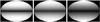Fig. 9 Brightness distribution on the stellar disk in the continuum at λ4437 Å, near the conspicuous He i 4471 Å line, calculated for a star rotating at η = 0.9 and for different values of α (from left to right): −1.0, 0.0 and 1.5, seen at an inclination angle of 90°.

5.1. The β exponent

The surface stellar brightness distributions are strongly dependent on the adopted darkening law. In the present discussion we write this law as follows: ${\mathit{F}}_{\mathrm{bol}}\mathrm{\left(}\mathit{\theta ,\alpha }\mathrm{\right)}\mathrm{=}\mathit{c}\mathrm{\left(}\mathit{\eta ,\alpha }\mathrm{\right)}{\mathit{g}}_{\mathrm{eff}}^{\mathrm{4}\mathit{\beta }}\mathrm{\left(}\mathit{\theta ,\alpha }\mathrm{\right)}\mathit{,}$(4)where ${\mathit{F}}_{\mathrm{bol}}\mathrm{\left(}\mathit{\theta ,\alpha }\mathrm{\right)}\mathrm{\propto }{\mathit{T}}_{\mathrm{eff}}^{\mathrm{4}}\mathrm{\left(}\mathit{\theta }\mathrm{\right)}$ is the local bolometric radiative flux and T_eff(θ) is the local effective temperature; c(η,α) is a function that should normally depend on both η and α, where α is the constant that parameterizes the degree of differential rotation, but in general possible also on θ. Here, η is the relation between the centrifugal acceleration at the equator (F_c) and the gravitational acceleration (F_g) at the equator, and α parameterizes the degree of surface differential rotation. We can assume that c is still a constant dependent only on η, but the effect of α passed entirely on β, which accordingly becomes β = β(α,β,θ). To put forward more clearly the effect of α, we adopt β to be constant and think of it as an average quantity over the co-latitude θ. To assess the influence of α on the stellar brightness distribution, we changed the surface effective gravity adopting the Maunder relation for the surface angular velocity $\mathrm{\Omega }\mathrm{\left(}\mathit{\theta }\mathrm{\right)}\mathrm{=}{\mathrm{\Omega }}_{\mathrm{eq}}\mathrm{(}\mathrm{1}\mathrm{+}\mathit{\alpha }{\cos }^{\mathrm{2}}{\mathit{\theta }}^{\mathrm{)}}\mathit{,}$(5)where Ω_eq is the angular velocity at the equator. For α > 0 the angular velocity is accelerated toward the pole (∂Ω/∂θ < 0; α can has any positive value), while for α < 0 angular velocity accelerates toward the equator (∂Ω/∂θ > 0; it must be α > −1.0 to keep all stellar latitudes rotating in the same sense). The fit of the solar surface differential angular velocity Ω(θ) law (Snodgrass 1984) with Eq. (5) produces α < −0.29 (Zorec et al. 2011). The expression for the effective gravity g_eff then becomes $\begin{array}{ccc}\begin{array}{c}\\ & & \\ & & \\ \end{array}\begin{array}{c}\mathrm{⎫}\\ \mathrm{⎪}\\ \mathrm{⎪}\\ \mathrm{⎪}\\ \mathrm{⎪}\\ \mathrm{⎪}\\ \mathrm{⎬}\\ \mathrm{⎪}\\ \mathrm{⎪}\\ \mathrm{⎪}\\ \mathrm{⎪}\\ \mathrm{⎪}\\ \mathrm{⎭}\end{array}& & \end{array}$ with $\mathit{\eta }\mathrm{=}\frac{{\mathit{F}}_{\mathrm{c}}}{{\mathit{F}}_{\mathrm{g}}}\mathrm{=}\frac{{\mathrm{\Omega }}_{\mathrm{eq}}^{\mathrm{2}}{\mathit{R}}_{\mathrm{eq}}^{\mathrm{3}}}{\mathit{G}{\mathit{M}}_{\mathit{\star }}}\mathrm{=}{\left(\frac{{\mathrm{\Omega }}_{\mathrm{eq}}}{{\mathrm{\Omega }}_{\mathrm{c}}}\right)}^{\mathrm{2}}{\left(\frac{{\mathit{R}}_{\mathrm{eq}}}{{\mathit{R}}_{\mathrm{c}}}\right)}^{\mathrm{3}}\mathrm{=}{\left(\frac{{\mathit{V}}_{\mathrm{eq}}}{{\mathit{V}}_{\mathrm{c}}}\right)}^{\mathrm{2}}\left(\frac{{\mathit{R}}_{\mathrm{eq}}}{{\mathit{R}}_{\mathrm{c}}}\right)\mathrm{·}$(6) In Eq. (6), r(θ) is the radius-vector normalized to the equatorial radius R_eq that describes the geometry of the stellar surface. In Eq. (6), g_p is the polar gravity; R_p and R_c are the polar and equatorial critical radii, respectively; M_⋆ is the stellar mass; V_eq and V_c are the equatorial linear velocity at η and critical velocity, respectively. The radius vector r(θ), radii R_p and R_eq must be calculated consistently as a function of η and α as indicated in Zorec et al. (2011). The effect in Eq. (6) of the centrifugal acceleration as a function of the co-latitude θ is produced by η_α(θ) and r(θ).

To see the influence of α on the stellar brightness distribution, we computed several maps with different values of η and α. The maps obtained for λ = 4437 Å, η = 0.9, β = 0.25, and for an object characterized by T_p = 19 000 K, log g_p = 4.0 seen at i = 90°, and several values of α are shown in Fig. 9. In Fig. 9, it is clearly apparent that in rapid rotators, α has a strong effect on the surface brightness distribution. Thus, even with the value of β = 0.25 (adopted for the calculations), the distribution of the surface brightness can be mis-interpreted in terms of apparent parameters, β_app ≠ β, if the original von Zeipel relation is used to account for the GDE. The apparent β_app can be estimated by dividing the stellar surface into elementary elements labeled with sub-indices (i,j) that indicate the respective co-latitude and longitude angles (θ_i,φ_j). Under the above adopted simplifications for the gravity darkening law, we let the parameter β vary over the stellar surface and adopted an average estimate of it, which is given by β_app = ⟨ β_i,j ⟩ ${\mathit{\beta }}_{\mathrm{app}}\mathrm{=}\mathrm{0.25}\mathrm{\times }\begin{array}{c}\mathrm{⎧}\\ \mathrm{⎪}\\ \mathrm{⎪}\\ \mathrm{⎪}\\ \mathrm{⎪}\\ \mathrm{⎨}\\ \mathrm{⎪}\\ \mathrm{⎪}\\ \mathrm{⎪}\\ \mathrm{⎪}\\ \mathrm{⎩}\end{array}\frac{\sum _{\mathit{i}\mathrm{=}\mathrm{1}}^{\mathit{n}}\sum _{\mathit{j}\mathrm{=}\mathrm{1}}^{\mathit{m}}\left\{\ln {\mathit{g}}_{\mathit{i,j}}^{\mathrm{\left(}\mathrm{0}\mathrm{\right)}}\mathrm{+}\ln \hspace{0.17em}\mathrm{[}{\mathit{F}}_{\mathit{i,j}}^{\mathrm{\left(}\mathit{\alpha }\mathrm{\right)}}\mathit{/}{\mathit{F}}_{\mathit{i,j}}^{\mathrm{\left(}\mathrm{0}\mathrm{\right)}}\mathrm{]}\right\}}{\sum _{\mathit{i}\mathrm{=}\mathrm{1}}^{\mathit{n}}\sum _{\mathit{j}\mathrm{=}\mathrm{1}}^{\mathit{m}}\ln {\mathit{g}}_{\mathit{i,j}}^{\mathrm{\left(}\mathit{\alpha }\mathrm{\right)}}}\begin{array}{c}\mathrm{⎫}\\ \mathrm{⎪}\\ \mathrm{⎪}\\ \mathrm{⎪}\\ \mathrm{⎪}\\ \mathrm{⎬}\\ \mathrm{⎪}\\ \mathrm{⎪}\\ \mathrm{⎪}\\ \mathrm{⎪}\\ \mathrm{⎭}\end{array}\mathrm{·}$(7) where ${\mathit{g}}_{\mathit{i,j}}^{\mathrm{\left(}\mathrm{0}\mathrm{\right)}}$, ${\mathit{g}}_{\mathit{i,j}}^{\mathrm{\left(}\mathit{\alpha }\mathrm{\right)}}$ are the effective gravities at (θ_i,φ_j) for α = 0 and α ≠ 0, respectively; while ${\mathit{F}}_{\mathit{i,j}}^{\mathrm{\left(}\mathrm{0}\mathrm{\right)}}$, ${\mathit{F}}_{\mathit{i,j}}^{\mathrm{\left(}\mathit{\alpha }\mathrm{\right)}}$ are the corresponding bolometric radiative fluxes. Table 4 summarizes the values of the apparent β_app calculated for the stellar example presented in Fig. 9, except that calculations were made for several values of η

From Table 4 we can see that β_app ≳ 0.25 when α ≲ 0.0 and β_app ≲ 0.25 if α ≳ 0.0. The higher the value of η, the larger the differences between β_app and β. These results show that the interpretation of β_app deduced from observations deserves a thorough discussion before anything can be said regarding the law characterizing the stellar surface rotation, whether radiation or convection prevails on the stellar surface. All these calculations rely on the assumption that the stellar atmosphere is in radiative equilibrium and that the radiative flux responds to the temperature gradient as established by the diffusion approximation. Claret (2012) has shown, however, that this approximation may not hold. Under more detailed representations of the radiative flux we can also have a β_app ≲ 0.25 effect that certainly relates in some way to the changes foreseen above as a function of α and β.

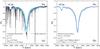Fig. 10 Rotationally broadened Hα line profiles using the fundamental parameters of α Cep and assuming rigid rotation. a) Line profiles adopting η = 0.57 (or Veq = 267 km s-1) and varying the inclination angle. For comparison sake, we have included the observed Hα line profile of α Cep. b) Line profiles adopting Veqsini = 225 km s-1 and varying η (or the inclination angle i).

5.2. The Hα line as a function of the inclination angle i and differential rotation parameter α

Because we have at our disposal interferometric observations covering almost the entire Hα line of α Cep, in the present section, we explore whether we can use this line to estimate the inclination angle i of the rotation axis. Knowing that the inclination angle is in principle a parameter of extrinsic character, it may be interesting to inquire on how much its determination may depend on the simultaneous knowledge of other intrinsic stellar quantities. A thorough discussion of this question is far beyond the scope of the present paper. We shall, however, briefly skim its dependence on the inclination angle i and on the differential rotation parameter α.

First, we calculated the Hα line emitted by the i-apparent stellar hemisphere by considering the stellar geometry controlled by a given η and several values of the differential rotation parameter α. Using the stellar geometry derived according to the rules given in Zorec et al. (2011), we assumed that each surface element is characterized by a plane-parallel stellar atmosphere corresponding to log g_eff(θ), and T_eff(θ) derived from Eq. (4). All these requirements are taken into account in the calculation code FASTROT modified for surface differential rotation (Frémat et al. 2005; Zorec et al. 2011). Adopting the stellar fundamental parameters of α Cep obtained by Zhao et al. (2009), we calculated two series of Hα line profiles assuming rigid rotation, i.e., α = 0.0. In the first series, shown in Fig. 10, we adopted V_eq = 267 km s^-1 ≈ [225 ± 20] /sin [55.7° ± 6.2°] which implies η ≃ 0.57, and varied the inclination angle in the interval 35° < i < 90°. In this figure we clearly see the very low sensitivity of the Hα line profile to the Vsini parameter. In the second series, also shown in Fig. 10, we have adopted Vsini = 225 km s^-1 and varied the force-ratio in the interval 0.4 < η < 0.8, which implies a change in the inclination angle from 46.7° to 77.1°.

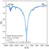Fig. 11 Rotationally broadened Hα line profiles using the fundamental parameters of α Cep and surface differential rotation. The line profiles are plotted for η = 0.57, Vsini = 225 km s-1 and for several values of α of the Maunder relation for surface differential rotation.

We see again that only the core of the line profile may show some significant changes as a function of η. For a third series of Hα line profiles we assumed η = 0.57 for the rotation at the equator, so that Vsini = 225 km s^-1 suited for i ≃ 56° and adopted several values of the differential parameter in the interval = −1.0 < α < +1.5. The line profiles obtained are shown in Fig. 11, where we see that once a Vsini is adopted, the core of the line changes somewhat with α.

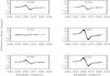Fig. 12 Estimated variations of the differential phases as function of the inclination (from 47.7° to 75.7°) of α Cep across the Hα line for our six observations. Calculations were performed with PA = −158°.

In a second step, we calculated brightness distributions over the apparent stellar hemisphere in the wavelengths of the Hα line by considering that the stellar geometry is controlled by a given η and differential rotation parameters α, seen at various inclination angles. The respective differential phases as a function of the wavelength λ inside the Hα line were calculated as before, with the physical parameters T_p, log g_p, Ω/Ω_c, R_eq/R_p, R_p/R_⊙, and β of α Cep found by Zhao et al. (2009) (see Table 1). We also considered the position angles or arrays during the observations carried out on α Cep from 2008 to 2010 and the corresponding baselines of VEGA/CHARA given in Table 2. For each baseline configuration and inclination angles i ranging from 47.7° to 75.7° by a 3° step, we obtained the differential phases shown in Fig. 12. If the method were sensitive enough to the inclination i, the interval chosen for the tested inclination angle i would, in principle, enable us to distinguish between the estimates of i by van Belle et al. (2006) and Zhao et al. (2009). The respective largest amplitudes of deviations of φ_diff(λ) obtained are given in Table 5, which show that for the configurations of the interferometric array used, our observations of the Hα line can hardly lead to conclusive results.

In spite of these results, we repeated the calculation of differential phases for a CHARA Array optimal configuration, represented by a baseline of 63 meters and position angle PA = 157°. Using the same stellar physical parameters and inclination angles 0° ≤ i ≤ 90° as before, we obtained the differential phases shown in Fig. 13. In the left panel are shown differential phases when Vsini = 225 km s^-1 is conserved and the inclination angle varied from in the interval 35° < i < 90°. We can see in this figure that the maximum amplitude of the phase variation is slightly larger than the uncertainty on the observational differential phase estimate (σ_φ ≃ 3°). In the left panel, models keep V(= 267 km s^-1) constant but vary the inclination angle from i = 0° to i = 90°. Since this is another diagnostic way to interpret the observed differential phases, we see that the method leads to amplitude changes of phases that are larger than Δφ = 5 × σ_φ. We also note that changes are also seen in the position of maxima larger than 10 km s^-1, which provide a supplementary tool for interpreting the observations. We may then expect that observations carried on the Hα line might lead us to some estimate of the inclination angle i if they are performed at optimal conditions, which unfortunately were not fulfilled in the present case. Finally, we note that model calculations should be made with fundamental parameters corresponding to the parent, non-rotating object. This implies that the estimate of i, α, and of the remaining stellar fundamental parameters have to be iterated. These problems will be discussed in greater detail in a forthcoming paper.

5.3. Properties of spectral lines and the determination of i and α

To understand better the lack of results on i and α obtained for α Cep from studies based on the Hα line, we considered the rotational broadening and differential phases as generalized convolutions between the line flux profile and a rotational broadening-like (RB) function. To this end, we note that the width of the rotational broadening function proper is about Δλ_RB = λ_HαVsini/c = 5.6 Å, while the Hα line spreads over some Δλ_Hα ≃ 80 Å. This means that the several intervening rotational broadening functions used should also behave like quasi-delta functions that nearly preserve the shape of the original spectral line profile, except perhaps in the line core wavelengths. Because the broad width of the Hα line is due to the Stark effect, to obtain more detailed information on the rotational broadening, in particular that produced by a surface differential rotation, spectral lines as free as possible from Stark broadening should be employed.The Hα line wings are sensitive to log   g, so a variation of the line profile in rapidly rotating stars induced by the θ-dependent log   g_eff is expected. Nevertheless, the rapidly rotating equatorial regions where both log   g_eff and the effective temperature are low do not contribute efficiently to the global line flux. The Doppler broadening of the line is thus left to the higher stellar latitudes where log   g_eff is comparatively larger and more uniform.

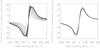Fig. 13 Differential phases φdiff(λ) over the Hα line for different inclination angles i of α Cep. Computations were done for a baseline of 63 m and baseline orientation −158°. Left panel: differential phases for Vsini = 225 km s-1 fixed, but varying inclination angle from i = 35° to i = 90° by steps Δi = 5° and η accordingly. Right panel: differential phases for V = 267 km s-1 fixed (η = 0.57) and inclination angles varying from i = 10° to i = 90° by steps Δi = 5°. The parent star without rotation has Teff = 7500 K and log g = 4.0.

Finally, the nature of the Hα line source function also deserves some attention. In stars with T_eff ≳ 8000 K, the Hα-source function is dominated by photo-ionizations, which make the line quite non-local in character (Thomas 1965, 1983; Mihalas 1978). Consequently, the Hα line formation is fairly independent of details concerning the non-uniform distributions of T_eff(θ) and log g_eff(θ) induced by the GDE. Because we expect that the surface differential rotation is correlated with physical condition changes in the line formation regions, to increase the degree of information on the external rotation law of stars, we should use spectral lines that not only carry signatures of the macroscopic broadening velocity fields, but also have source functions sensitive to changes of local physical conditions (T_e,N_e). This means that these spectral lines should have source functions that are collision-dominated.

5.4. Information expected from spectral lines sensitive to effects induced by the rotation

According to spectral type and luminosity class, several spectral lines can be good candidates to carry out such studies. Since the identification of these lines and the subsequent calculation of expected effects from all of them is far beyond the scope of the present paper, we limit our discussion to a hypothetical line that behaves like the He iλ 4471 line, which fulfills the above quoted requirements in stars with T_eff ≳ 10 000. Though this line is not useful for α Cep, our aim is to briefly sketch some expected effects of quite general character.

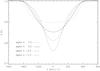Fig. 14 He i 4471-like line profiles as a function of different values of the differential rotation parameter α. The star is characterized by Tp = 19 000 K, log gp = 4.0, η = 0.9, β = 0.25 and i = 45°.

Because the He iλ 4471 line is only a hypothetical model line, we do not proceed with detailed radiation transfer calculations, but represent the emergent monochromatic specific intensity I(λ,μ) directed toward the observer as follows: $\mathit{I}\mathrm{\left(}\mathit{\theta ,\phi ,\eta ,\alpha ,\lambda ,\mu }\mathrm{\right)}\mathrm{=}\mathit{H}\left[\mathit{\theta ,\lambda }\mathrm{-}{\mathit{\lambda }}_{\mathit{o}}\frac{{\mathit{V}}_{\mathrm{proj}}\mathrm{\left(}\mathit{\theta ,\phi ,\alpha ,i}\mathrm{\right)}}{\mathit{c}}\right]{\mathit{I}}_{\mathrm{c}}\mathrm{\left(}\mathit{\theta ,\eta ,\alpha ,\mu }\mathrm{\right)}\mathit{,}$(8) where θ reflects the dependence of I(λ,μ) with the local T_eff(θ) and log g_eff(θ), whose variation with θ is determined by η and α; the dependence of I(λ,μ) with the longitude φ is due to the law of the surface differential rotation that produces iso-radial velocity curves that are a function of θ and φ over the apparent stellar hemisphere; η controls the equatorial rotational velocity, and α parameterizes the surface differential rotation according to the Maunder law; I_c(θ,η,α,μ) is the specific radiation intensity directed toward the observer in the continuum at the central wavelength λ_c of the studied line; , where $\mathit{n̂}\mathrm{=}{\overline{\mathit{g}}}_{\mathrm{eff}}\mathrm{\left(}\mathit{\theta }\mathrm{\right)}\mathit{/}\mathrm{\left|}{\mathit{g}}_{\mathrm{eff}}\mathrm{\right(}\mathit{\theta }\mathrm{\left)}\mathrm{\right|}$ and cosiê_y +siniê_z are the unit normal vector to the stellar surface and the unit vector directed toward the observer, respectively. The specific intensity I_c is represented as ${\mathit{I}}_{\mathrm{c}}\mathrm{\left(}\mathit{\theta ,\eta ,\alpha ,\mu }\mathrm{\right)}\mathrm{=}\frac{{\mathit{F}}_{\mathrm{c}}\mathrm{\left(}\mathit{\theta }\mathrm{\right)}}{\mathit{\pi }\left(\mathrm{1}\mathrm{-}{\mathit{ϵ}}_{{\mathit{\lambda }}_{\mathrm{c}}}\mathit{/}\mathrm{3}\right)}\mathrm{(}\mathrm{1}\mathrm{-}{\mathit{ϵ}}_{{\mathit{\lambda }}_{\mathrm{c}}}\mathrm{+}{\mathit{ϵ}}_{{\mathit{\lambda }}_{\mathrm{c}}}\cos \mathit{\mu }\mathrm{)}\mathit{,}$(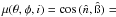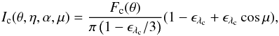9) where F_c(θ) is the emergent continuum radiation flux λ_c at λ_c; ϵ_λc is the limb darkening coefficient ϵ_λ at λ_c of the continuum spectrum that we interpolated in Claret (2012) for the solar chemical abundance and the local [T_eff(θ),log g_eff(θ)]. In a more detailed treatment of spectral lines, the limb darkening coefficient should vary with the wavelength inside the spectral line (Collins & Truax 1995; Chauville et al. 2001).

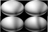Fig. 15 Iso-radial velocity zone for λ = 4438.78 Å. Top, form left to right: α = −1.0 and −0.5. Bottom, from left to right: α = 0.0 and 1.0. computations were done for an inclination angle of i = 45°.

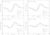Fig. 16 Evolution of the differential phase as a function of the wavelength through the He i line for different values of α. Differential phases were computed for different orientations and a 60-m baseline. The position angle of the star is assumed to be equal to zero, the inclination angle of the rotation axis is i = 45°, and the stellar angular diameter is assumed to be 1.3 mas.

Let (x,y,z) be a Cartesian reference system centered on the apparent stellar disk, where (x,y) are in the plane of the sky, z is directed towards the observer, y is in the plane containing z and the stellar rotation axis. The radial velocity projected towards the observer of a surface point (r,θ,φ) is then $\begin{array}{c}\\ {\mathit{V}}_{\mathrm{proj}}\mathrm{\left(}\mathit{\theta ,\phi ,\eta ,\alpha ,i}\mathrm{\right)}& \mathrm{=}& \mathrm{[}\overline{\mathrm{\Omega }\mathrm{\left(}\mathit{\theta }\mathrm{\right)}}\mathrm{\wedge }{\overline{{r}\mathrm{\left(}\mathit{\theta ,\eta ,\alpha }\mathrm{\right)}}}^{\mathrm{]}}\mathit{.}\mathrm{ß̂}\\ & \mathrm{=}& \mathrm{\Omega }\mathrm{\left(}\mathit{\theta ,\alpha }\mathrm{\right)}{\mathit{R}}_{\mathrm{eq}}\mathrm{\left(}\mathit{\eta }\mathrm{\right)}\mathit{x}\mathrm{\left(}\mathit{\eta ,\theta ,\phi }\mathrm{\right)}\sin \mathit{i}\\ \mathit{x}\mathrm{\left(}\mathit{\eta ,\theta ,\phi }\mathrm{\right)}& \mathrm{=}& {r}\mathrm{\left(}\mathit{\theta ,\eta ,\alpha }\mathrm{\right)}\sin \mathit{\theta }\sin \mathit{\phi ,}\end{array}\begin{array}{c}\mathrm{⎫}\\ \mathrm{⎪}\\ \mathrm{⎪}\\ \mathrm{⎪}\\ \mathrm{⎪}\\ \mathrm{⎬}\\ \mathrm{⎪}\\ \mathrm{⎪}\\ \mathrm{⎪}\\ \mathrm{⎪}\\ \mathrm{⎭}\end{array}$(10) where Ω(θ,α) is given by Eq. (5); i is the inclination angle of the stellar rotation axis; r(θ,η,α) is the radius vector a point in the stellar surface.

The calculation of the flux line profile F(λ) was made as in all preceding calculations: the star was divided into surface elements to which were associated with the respective T_eff(θ), log g_eff(θ) and V_proj(θ,φ,α,i) that enable one to obtain the local Doppler-shifted specific intensity directed toward the observer. The integration over the visible stellar hemisphere of the projected specific intensities produces F(λ). The central intensity and equivalent widths dependent on [T_eff,log g_eff] needed to determine the intrinsic line profile H(λ) lower case In Eq. (8) were taken from Frémat et al. (2005). Equation (9) was used to obtain the local specific radiation intensity, either monochromatic or bolometric, directed toward the observer, which determines the sought distribution of the surface brightness. For the test examples calculated here, the input parameters were the polar effective temperature T_p = 19 000 K, the polar gravity g_p = 4.0, the inclination angle i = 45°, gravity darkening exponent of the gravity darkening law β = 0.25, the ratio η = 0.9, and several values of the differential rotation parameter α. The test He iλ4471 line-like profiles obtained are shown in Fig. 14, where the strong variation of the line profiles according to the value of α is clearly apparent.

The corresponding maps of brightness distribution containing the iso-radial velocity zone for λ = 4439 Å, calculated for the same fundamental parameters, are shown in Fig. 15. At the top of this figure, from left to right, the images are for α = −1.0 and −0.5, while in the bottom panels we have from left to right, α = 0.0 and 1.0. We can clearly see in this figure that the regions crossed by a given iso-radial velocity curve are quite different. The iso-radial velocity curves thus run across zones with different (T_eff,log g) contributing to the final line flux profile with local line profiles having different intensities and Doppler broadenings. In Fig. 16 we note that according to the parameter α, not only the amplitude variations of differential phase are stronger than the expected uncertainties affecting the observed differential phases, but the strongest phase deviations are radial-velocity shifted, which are α −dependent. In this figure we notice that deviations of maxima in the differential phases exceed 10 km s^-1 and the amplitude variation of this maximum widely exceeds 3°. These limits correspond to the VEGA/CHARA sensitivity. A spectral line in α Cep that would behave like the witness spectral line treated here could lead us to reliable inferences of the differential parameter α. Looking for appropriate configurations of the interferometric array might improve the estimates even more.

6. Conclusions

Differential phases in the Hα line of α Cep observed during six observations at the VEGA/CHARA array in September 2008 and October 2010 were presented. We successfully applied a method for determining the position angle of the rotationally deformed star that takes advantage of the differential phases obtained at different configurations of the interferometric array, and is independent of the knowledge of the stellar fundamental parameters. We have thus obtained $\mathrm{PA}\mathrm{=}\mathrm{-}\mathrm{15}{\mathrm{7}}_{\mathrm{-}\mathrm{10}°}^{\mathrm{+}\mathrm{17}°}$.

We discussed the feasibility of determining differential phases using the gravity darkening exponent β in von Zeipel’s relation, the inclination angle i of the star, and the differential rotation parameter α of Maunders’s expression for the stellar surface rotation law. The discussion showed that the exponent β is a function of the rotation rate η = F_c/F_g (F_c = centrifugal acceleration at the equator; F_g = gravitational acceleration) and of α. Its determination is probably not straightforward and needs a careful discussion of interferometric imaging of stellar surfaces.

From models of the Hα emitted by a rapidly rotating star with the fundamental parameters α Cep, we showed that for very ideal configurations of interferometric arrays it would be possible to estimate the inclination angle i. Nevertheless, a knowledge of the stellar fundamental parameters is needed. They can be inferred by iteration together with the inclination angle i. We finally concluded that spectral lines that are not strongly affected by Stark broadening and have collision-dominated source functions should be observed to estimate i and α with differential phases. They are sensitive to these quantities in three different ways: height of the deviation wings, the value of the maximum deviation, and the spectral position of the maximum deviation.

Acknowledgments

VEGA is a collaboration between CHARA and OCA/LAOG/CRAL/LESIA that has been supported by the French programs PNPS and ASHRA, by INSU and by the Région PACA. The project has obviously benefitted from the strong support of the OCA and CHARA technical teams. The CHARA Array is operated with support from the National Science Foundation through grant AST-0908253, the W. M. Keck Foundation, the NASA Exoplanet Science Institute, and from Georgia State University. This work has made use of the BeSS database, operated at GEPI, Observatoire de Meudon, France: http://basebe.obspm.fr, use of the Jean-Marie Mariotti Center SearchCal service¹ co-developed by FIZEAU and LAOG, and of CDS Astronomical Databases SIMBAD and VIZIER². We are grateful to an anonymous referee for her/his valuable suggestions that helped to improve the presentation of our results.

References

All Tables

All Figures

	Fig. 1 (u,v)-plane coverage by our observations (u is in abscissas).
In the text

	Fig. 2 Differential phases obtained after data processing. This figure also shows the best-fit (red line) models calculated as a function of the position angle of the rotation axis ($\mathrm{PA}\mathrm{=}\mathrm{-}\mathrm{15}{\mathrm{7}}_{\mathrm{-}\mathrm{10}°}^{\mathrm{+}\mathrm{17}°}$) obtained as explained in Sect. 4.4.
In the text

Fig. 3 Top: intensity maps calculated for selected wavelengths inside the Hα line (from left to right): 6559.5 Å, 6561.3 Å, 6562.8 Å, and 6565.2 Å. Ordinates and abscissas are given in units of the equatorial radius Req. The inclination angle used is i = 55°. Bottom: photo-center displacements along the y-axis (left side); differential phase associated with the photo-center shift (right side). All quantities are computed for a sixty-meter baseline parallel to the equatorial axis (x-axis). The photo-center displacements are given in units of the angular stellar radius.

In the text

Fig. 4 Differential phases φdiff(λ) in the Hα line for different baseline orientations. Top: stellar disk deformed by the fast rotation and projected onto the sky where we have represented the baseline orientations: 0° (cross), 45° (star), 90° (solid line) and 160° (diamond). Bottom: evolution of φdiff(λ) according to the baseline orientations represented on top and computed for a sixty meter-baseline. In this example we assumed that the position angle of the stellar rotation axis is equal to zero.

In the text

	Fig. 5 Spectrum of alpha Cep obtained in the high spectral resolution mode of VEGA/CHARA (green) and ith the ELODIE spectrograph (red).
In the text

	Fig. 6 Surface brightness distribution in α Cep at four different wavelengths: 6548.7 Å (top, left), 6557.7 Å (top, right), λ6562.8 Å (bottom, left), and λ6568.5 Å, (bottom, right). Ordinates and abscissas are given in units of the equatorial radius Req. The inclination angle used is i = 55°.
In the text

	Fig. 7 ${\mathit{\chi }}_{\mathrm{red}}^{\mathrm{2}}$ as a function of the PA of the rotation axis of α Cep for different von Zeipel exponents ranging from β = 0.08 to β = 0.25.
In the text

	Fig. 8 a) Simulated position angle PA against the number of “bootstrap” replications when β = 0.19. The colored line indicates the position angle PA of maximum probability. b) Frequency distribution of the simulated position angles PA (histogram and smoothed distribution). In the figure are also indicated the position angle PA of maximum probability and the 99% confidence interval.
In the text

	Fig. 9 Brightness distribution on the stellar disk in the continuum at λ4437 Å, near the conspicuous He i 4471 Å line, calculated for a star rotating at η = 0.9 and for different values of α (from left to right): −1.0, 0.0 and 1.5, seen at an inclination angle of 90°.
In the text

	Fig. 10 Rotationally broadened Hα line profiles using the fundamental parameters of α Cep and assuming rigid rotation. a) Line profiles adopting η = 0.57 (or Veq = 267 km s-1) and varying the inclination angle. For comparison sake, we have included the observed Hα line profile of α Cep. b) Line profiles adopting Veqsini = 225 km s-1 and varying η (or the inclination angle i).
In the text

	Fig. 11 Rotationally broadened Hα line profiles using the fundamental parameters of α Cep and surface differential rotation. The line profiles are plotted for η = 0.57, Vsini = 225 km s-1 and for several values of α of the Maunder relation for surface differential rotation.
In the text

	Fig. 12 Estimated variations of the differential phases as function of the inclination (from 47.7° to 75.7°) of α Cep across the Hα line for our six observations. Calculations were performed with PA = −158°.
In the text

Fig. 13 Differential phases φdiff(λ) over the Hα line for different inclination angles i of α Cep. Computations were done for a baseline of 63 m and baseline orientation −158°. Left panel: differential phases for Vsini = 225 km s-1 fixed, but varying inclination angle from i = 35° to i = 90° by steps Δi = 5° and η accordingly. Right panel: differential phases for V = 267 km s-1 fixed (η = 0.57) and inclination angles varying from i = 10° to i = 90° by steps Δi = 5°. The parent star without rotation has Teff = 7500 K and log g = 4.0.

In the text

	Fig. 14 He i 4471-like line profiles as a function of different values of the differential rotation parameter α. The star is characterized by Tp = 19 000 K, log gp = 4.0, η = 0.9, β = 0.25 and i = 45°.
In the text

	Fig. 15 Iso-radial velocity zone for λ = 4438.78 Å. Top, form left to right: α = −1.0 and −0.5. Bottom, from left to right: α = 0.0 and 1.0. computations were done for an inclination angle of i = 45°.
In the text

	Fig. 16 Evolution of the differential phase as a function of the wavelength through the He i line for different values of α. Differential phases were computed for different orientations and a 60-m baseline. The position angle of the star is assumed to be equal to zero, the inclination angle of the rotation axis is i = 45°, and the stellar angular diameter is assumed to be 1.3 mas.
In the text

References

- Abt, H. A., & Morrell, N. I. 1995, ApJS, 99, 135 [Google Scholar]
- Aufdenberg, J. P., Mérand, A., Coudé du Foresto, V., et al. 2006, ApJ, 645, 664 [NASA ADS] [CrossRef] [Google Scholar]
- Berio, P., Mourard, D., Bonneau, D., et al. 1999, J. Opt. Soc. Am. A, 16, 872 [NASA ADS] [CrossRef] [Google Scholar]
- Bernacca, P. L., & Perinotto, M. 1973a, in Main sequence single stars, A catalogue of stellar rotational velocities (Universita di Padova), 1 [Google Scholar]
- Bernacca, P. L., & Perinotto, M. 1973b, in Main sequence spectroscopic binaries, A catalogue of stellar rotational velocities (Universita di Padova), 2 [Google Scholar]
- Bernacca, P. L., & Perinotto, M. 1973c, in Evolved stars, A catalogue of stellar rotational velocities (Universita di Padova), 4 [Google Scholar]
- Bowman, A. W., & Azzalini, A. 1997, Applied smoothing techniques for data analysis: the kernel approach with S-plus illustrations, Oxford statistical science series No. 18 (Clarendon Press) [Google Scholar]
- Chauville, J., Zorec, J., Ballereau, D., et al. 2001, A&A, 378, 861 [NASA ADS] [CrossRef] [EDP Sciences] [Google Scholar]
- Che, X., Monnier, J. D., Zhao, M., et al. 2011, ApJ, 732, 68 [NASA ADS] [CrossRef] [Google Scholar]
- Claret, A. 2012, A&A, 538, A3 [NASA ADS] [CrossRef] [EDP Sciences] [Google Scholar]
- Collins, II, G. W., & Truax, R. J. 1995, ApJ, 439, 860 [NASA ADS] [CrossRef] [Google Scholar]
- Domiciano de Souza, A., Vakili, F., Jankov, S., Janot-Pacheco, E., & Abe, L. 2002, A&A, 393, 345 [NASA ADS] [CrossRef] [EDP Sciences] [Google Scholar]
- Domiciano de Souza, A., Kervella, P., Jankov, S., et al. 2003, A&A, 407, L47 [NASA ADS] [CrossRef] [EDP Sciences] [Google Scholar]
- Domiciano de Souza, A., Hadjara, M., Vakili, F., et al. 2012a, A&A, 545, A130 [NASA ADS] [CrossRef] [EDP Sciences] [Google Scholar]
- Domiciano de Souza, A., Zorec, J., & Vakili, F. 2012b, SF2A Proc., in press [Google Scholar]
- Douglas, A. V. 1926, ApJ, 64, 262 [NASA ADS] [CrossRef] [Google Scholar]
- Efron, B., & Tibshirani, R. 1986, Statist. Sci., 1, 54 [Google Scholar]
- Endal, A. S., & Sofia, S. 1979, ApJ, 232, 531 [NASA ADS] [CrossRef] [Google Scholar]
- Espinosa Lara, F., & Rieutord, M. 2012, A&A, 547, A32 [NASA ADS] [CrossRef] [EDP Sciences] [Google Scholar]
- Frémat, Y., Zorec, J., Hubert, A.-M., & Floquet, M. 2005, A&A, 440, 305 [NASA ADS] [CrossRef] [EDP Sciences] [Google Scholar]
- Gray, R. O., Corbally, C. J., Garrison, R. F., McFadden, M. T., & Robinson, P. E. 2003, AJ, 126, 2048 [NASA ADS] [CrossRef] [Google Scholar]
- Heger, A., & Langer, N. 2000, ApJ, 544, 1016 [NASA ADS] [CrossRef] [Google Scholar]
- Hubeny, I., & Lanz, T. 1995, ApJ, 439, 875 [Google Scholar]
- Johnson, H. L., & Morgan, W. W. 1953, ApJ, 117, 313 [NASA ADS] [CrossRef] [Google Scholar]
- Kervella, P., & Domiciano de Souza, A. 2006, A&A, 453, 1059 [NASA ADS] [CrossRef] [EDP Sciences] [Google Scholar]
- Kiziloglu, N., & Civelek, R. 1996, A&A, 307, 88 [NASA ADS] [Google Scholar]
- Kurucz, R. L. 1979, ApJS, 40, 1 [NASA ADS] [CrossRef] [Google Scholar]
- Lamers, H. J. G. L. M., & Cassinelli, J. P. 1999, Introduction to Stellar Winds (Cambridge University Press) [Google Scholar]
- Le Bouquin, J.-B., Absil, O., Benisty, M., et al. 2009, A&A, 498, L41 [NASA ADS] [CrossRef] [EDP Sciences] [Google Scholar]
- Lucy, L. B. 1967, ZAp, 65, 89 [NASA ADS] [Google Scholar]
- Maeder, A., Meynet, G., & Ekström, S. 2007, in From Stars to Galaxies: Building the Pieces to Build Up the Universe, eds. A. Vallenari, R. Tantalo, L. Portinari, & A. Moretti, ASP Conf. Ser., 374, 13 [Google Scholar]
- Maeder, A., Georgy, C., & Meynet, G. 2008, A&A, 479, L37 [NASA ADS] [CrossRef] [EDP Sciences] [Google Scholar]
- McAlister, H. A., ten Brummelaar, T. A., Gies, D. R., et al. 2005, ApJ, 628, 439 [NASA ADS] [CrossRef] [Google Scholar]
- Meynet, G., & Maeder, A. 2000, A&A, 361, 101 [NASA ADS] [Google Scholar]
- Mihalas, D. 1978, Stellar atmospheres, 2nd Ed. (San Francisco: W. H. Freeman and Co.) [Google Scholar]
- Monnier, J. D., Zhao, M., Pedretti, E., et al. 2007, Science, 317, 342 [NASA ADS] [CrossRef] [PubMed] [Google Scholar]
- Mourard, D. 1990, Ph.D. Thesis, Université de Nice [Google Scholar]
- Mourard, D., Clausse, J. M., Marcotto, A., et al. 2009, A&A, 508, 1073 [NASA ADS] [CrossRef] [EDP Sciences] [Google Scholar]
- Mourard, D., Tallon, M., Bério, P., et al. 2010, in SPIE Conf. Ser., 7734 [Google Scholar]
- Pinsonneault, M. H., Deliyannis, C. P., & Demarque, P. 1991, ApJ, 367, 239 [NASA ADS] [CrossRef] [Google Scholar]
- Reiners, A. 2003, A&A, 408, 707 [NASA ADS] [CrossRef] [EDP Sciences] [Google Scholar]
- Royer, F., Zorec, J., & Gómez, A. E. 2007, A&A, 463, 671 [NASA ADS] [CrossRef] [EDP Sciences] [Google Scholar]
- Sackmann, I. J. 1970, A&A, 8, 76 [NASA ADS] [Google Scholar]
- Shimazaki, H., & Shinomoto, S. 2007, Neural Computation, 19, 1503 [Google Scholar]
- Simon, T., & Landsman, W. B. 1997, ApJ, 483, 435 [NASA ADS] [CrossRef] [Google Scholar]
- Simon, T., Ayres, T. R., Redfield, S., & Linsky, J. L. 2002, ApJ, 579, 800 [NASA ADS] [CrossRef] [Google Scholar]
- Snodgrass, H. B. 1984, Sol. Phys., 94, 13 [NASA ADS] [CrossRef] [Google Scholar]
- Talon, S., Zahn, J.-P., Maeder, A., & Meynet, G. 1997, A&A, 322, 209 [NASA ADS] [Google Scholar]
- Tatulli, E., Millour, F., Chelli, A., et al. 2007, A&A, 464, 29 [NASA ADS] [CrossRef] [EDP Sciences] [Google Scholar]
- ten Brummelaar, T. A., McAlister, H. A., Ridgway, S. T., et al. 2005, ApJ, 628, 453 [NASA ADS] [CrossRef] [Google Scholar]
- Thomas, R. N. 1965, Some aspects of non-equilibrium thermodynamics in the presence of a radiation field (University of Colorado Press) [Google Scholar]
- Thomas, R. N. 1983, Stellar atmospheric structural patterns, 471 (NASA-CNRS) [Google Scholar]
- Townsend, R. H. D. 1997, MNRAS, 284, 839 [NASA ADS] [CrossRef] [Google Scholar]
- Tuominen, I. V. 1972, Ann. Acad. Sci. Fennicae, 392 [Google Scholar]
- Uesugi, A., & Fukuda, I. 1970, Catalogue of rotational velocities of the stars (University of Kyoto) [Google Scholar]
- van Belle, G. T., Ciardi, D. R., Thompson, R. R., Akeson, R. L., & Lada, E. A. 2001, ApJ, 559, 1155 [NASA ADS] [CrossRef] [MathSciNet] [Google Scholar]
- van Belle, G. T., Ciardi, D. R., ten Brummelaar, T., et al. 2006, ApJ, 637, 494 [NASA ADS] [CrossRef] [Google Scholar]
- von Zeipel, H. 1924, MNRAS, 84, 665 [NASA ADS] [CrossRef] [Google Scholar]
- Walter, F. M., Matthews, L. D., & Linsky, J. L. 1995, ApJ, 447, 353 [NASA ADS] [CrossRef] [Google Scholar]
- Zahn, J.-P. 1992, A&A, 265, 115 [NASA ADS] [Google Scholar]
- Zhao, M., Monnier, J. D., Pedretti, E., et al. 2009, ApJ, 701, 209 [NASA ADS] [CrossRef] [Google Scholar]
- Zorec, J., Frémat, Y., Domiciano de Souza, A., et al. 2011, A&A, 526, A87 [NASA ADS] [CrossRef] [EDP Sciences] [Google Scholar]
All Tables
Parameters from best models obtained by van Belle et al. (2006) and Zhao et al. (2009).
Strongest variation of φdiff(λ) across the Hα line of α Cep as a function inclination angles i ranging from 47.7° to i = −75.7°.