| Issue |
A&A
Volume 554, June 2013
|
|
|---|---|---|
| Article Number | A57 | |
| Number of page(s) | 6 | |
| Section | Astrophysical processes | |
| DOI | https://doi.org/10.1051/0004-6361/201321488 | |
| Published online | 05 June 2013 | |
Towards modeling quasi-periodic oscillations of microquasars with oscillating slender tori
1 N. Copernicus Astronomical Centre, ul. Rabiańska 8, 87-100 Toruń, Poland
e-mail: This email address is being protected from spambots. You need JavaScript enabled to view it.
2 Physics Department, Gothenburg University, 41296 Göteborg, Sweden
e-mail: This email address is being protected from spambots. You need JavaScript enabled to view it.
3 Physics Department, Warsaw University, ul. Moża 69, 00-681 Warsaw, Poland
e-mail: This email address is being protected from spambots. You need JavaScript enabled to view it.
4 Chalmers University of Technology, 41296 Gothenburg, Sweden
e-mail: This email address is being protected from spambots. You need JavaScript enabled to view it.
5 Physics Department, Silesian University, Opava, Czech Republic
e-mail: This email address is being protected from spambots. You need JavaScript enabled to view it.
, This email address is being protected from spambots. You need JavaScript enabled to view it.
, This email address is being protected from spambots. You need JavaScript enabled to view it.
Received: 15 March 2013
Accepted: 29 April 2013
Abstract
Context. One of the often discussed models for high-frequency quasi-periodic oscillations of X-ray binaries is the oscillating torus model, which considers oscillation modes of slender accretion tori.
Aims. Here, we aim at developing this model by considering the observable signature of an optically thick slender accretion torus subject to simple periodic deformations.
Methods. We compute light curves and power spectra of a slender accretion torus subject to simple periodic deformations: vertical or radial translation, rotation, expansion, and shear.
Results. We show that different types of deformations lead to very different Fourier power spectra and therefore could be observationally distinguished.
Conclusions. This work is a first step in a longer term study of the observable characteristics of the oscillating torus model. It gives promising perspectives on the possibility of constraining this model by studying the observed power spectra of quasi-periodic oscillations.
Key words: accretion, accretion disks / black hole physics / relativistic processes
© ESO, 2013
1. Introduction
Some microquasars exhibit high-frequency (millisecond) quasi-periodic oscillations (QPOs), which in this work always refer to high-frequency oscillations; low-frequency QPOs are not considered here. These high-frequency oscillations are characterized by a narrow peak in the source power spectrum (see van der Klis 2004; Remillard & McClintock 2006, for a review). As the timescale of this variability is of the same order as the Keplerian orbital period at the innermost stable circular orbit of the central black hole, it is highly probable that these phenomena are linked with strong-field general relativistic effects. The other different low-mass X-ray binaries that contain neutron stars display QPOs on these prominent timescales as well. There is no consensus on the possible QPO origin and uniformity across different sources yet.
A variety of models have been developed so far to account for the high-frequency variability. Stella & Vietri (1999) and Stella et al. (1999) suggest that QPOs could arise from the modulation of the X-ray flux by the periastron precession and the Keplerian frequency of blobs of matter orbiting in an accretion disk around the central compact object. Also, QPOs could be due to modulation of the X-ray flux by oscillations of a thin accretion disk surrounding the central compact object (see Wagoner 1999; Kato 2001). Fragile et al. (2001) propose that QPOs are due to the modulation of the X-ray flux caused by a warped accretion disk surrounding the central compact object. Pointing out the 3:2 ratio of some QPOs in different sources, Abramowicz & Kluźniak (2001) have proposed a resonance model in which these pairs of QPOs are due to the beat between the Keplerian and epicyclic frequencies of a particle orbiting around the central compact object.
General relativistic ray tracing of radiating or irradiated hot spots orbiting around black holes and neutron stars was founded at the turn of the millennium. For instance, Karas (1999) discusses already sophisticated numeric modeling of observable modulation from clumps distributed around certain preferred circular orbits. Later, Schnittman & Bertschinger (2004) investigated in great detail predictions of a model of hot spot radiating isotropically on nearly circular equatorial orbits. In their study, the hypothetic resonance between the Keplerian and radial epicyclic frequencies gives rise to peaks in the modeled power spectrum. Tagger & Varnière (2006) advocate the fact that QPOs in microquasars are due to the triggering of a Rossby wave instability in the accretion disk surrounding the central compact object. Ray-traced light curves have been recently developed for this model by Vincent et al. (2013). Finally, models involving oscillations of accretion tori have been developed. As our work is a follow-up of these past studies, we present them in more details.
The first study of a QPO model involving thick accretion structure (tori) was developed by Rezzolla et al. (2003), who showed that p-mode oscillation of a numerically computed accretion torus can generate QPOs. Ray-traced light curves and power spectra of this model were derived by Schnittman & Rezzolla (2006). The analysis of analytical accretion tori (for which all physical quantities are known analytically throughout the structure and at all times) as a model for QPOs was initiated by Bursa et al. (2004), who performed simulations of ray-traced light curves and power spectra of an optically thin oscillating slender torus. This model took only into account simple vertical and radial sinusoidal motion of a circular cross-section torus. To allow a more general treatment, a series of theoretical works were dedicated to developing a proper model of general oscillation modes of a slender or non-slender perfect-fluid hydrodynamical accretion torus (Abramowicz et al. 2006; Blaes et al. 2006; Straub & Šrámková 2009). Considering hydrodynamical perfect-fluid tori is interesting in terms of simplicity as all computations can be derived analytically and all physical quantities are known analytically at all times.
The aim of this article is to strengthen the perfect-fluid oscillating slender torus model for QPOs by progressing towards determining its observable signature. Here, we present a first step towards this goal, which consists of determining the observable signature of simple deformations of a slender torus in the Schwarzschild metric. We do not use the mathematically well-defined oscillation formalism derived by Blaes et al. (2006). We rather consider the impact on the observables of elementary deformations of the torus cross-section: translation, rotation, expansion, and shear. We simulate light curves and power spectra of such tori subject to these simple deformations, taking into account all relativistic effects that will affect radiation by using a ray-tracing code. The focus of this article is thus to determine the impact of the geometrical change of a slender torus on the observed flux variation. We do not consider the physics of the matter forming the torus.
This model is extremely simple and does not claim to give a realistic view of the nature of QPOs. However, it does allow determination in the simplest possible framework of whether different kinds of motions of a toroidal accretion structure lead to potentially observable differences in the light curves. This work thus makes it possible to go one step further in the development of the oscillating torus model for QPOs.
Section 2 describes the equilibrium slender torus, while Sect. 3 describes its deformations in terms of translation, rotation, expansion, and shear. Section 4 shows the ray-traced light curves and power spectra of the deformed torus, and Sect. 5 gives conclusions and prospects.
2. Equilibrium of a slender accretion torus
This section derives the equations that describe the accretion torus at equilibrium. The spacetime is described by the Schwarzschild metric in the Schwarzschild coordinates (t,r,θ,ϕ), with geometrical units c = 1 = G and signature (− , + , + , +). The line element has then the following form: 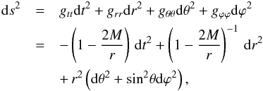 (1)where M is the black hole mass. In the remaining article, we use units where this mass is 1.
In this spacetime, we consider an axisymmetric, non-self-gravitating, perfect fluid, constant specific angular momentum, which circularly orbits the accretion torus. This torus is assumed to be slender, meaning that its cross section is small as compared to its central radius.
2.1. Fluid motion
As the fluid follows circular geodesics, its 4-velocity can be written as 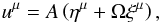 (2)where Ω is the fluid’s angular velocity, and ημ and ξμ are the Killing vectors associated with stationarity and axisymmetry, respectively. The constant A is given by imposing the normalization of the 4-velocity, uμuμ = − 1.
As spacetime is stationary and axisymmetric, the specific energy ℰ and specific angular momentum ℒ are defined as 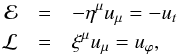 (3)which are geodesic constants of motion.
The rescaled specific angular momentum ℓ is defined according to 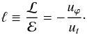 (4)We assume this rescaled specific angular momentum to be constant throughout the torus:
  (5)The 4-acceleration along a given circular geodesic followed by the fluid is
  (6)where
  is the effective potential (see, e.g., Abramowicz et al. 2006):
  (7)The radial and vertical epicyclic frequencies for circular motion are related to the second derivatives of this potential:
  (8)In the Schwarzchild metric, these epicyclic frequencies at the torus center are
  (9)where a subscript 0 denotes here and in the rest of this article a quantity evaluated at the torus center. The Keplerian angular velocity is well known:
  .
.
In the rest of this article, the torus central radius will be fixed to the value r0, satisfying the following condition  (10)This choice is linked to our goal of applying the deformed torus model to twin-peak QPOs. It results in
  (11)
(11)
2.2. Surface function
Following Abramowicz et al. (2006), we define the surface of the torus by the locus of the zeros of a surface function f(r,θ). Introducing the following set of coordinates 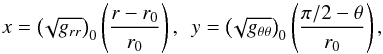 (12)Abramowicz et al. (2006) show that the surface function is expressed according to
 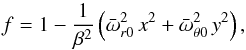 (13)where
 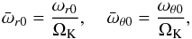 (14)the parameter β is related to the torus thickness, and the torus being slender:
  (15)Abramowicz et al. (2006) also show that the x and y coordinates are of order β. We thus define a new set of order-unity coordinates:
  (16)and:
  (17)The equilibrium slender torus has therefore an elliptical cross section.
3. Deformations of a slender accretion torus
This section is devoted to determining the surface function of the torus subject to simple deformations: translation, rotation, expansion, and shear. The 4-velocity of the perturbed fluid is also given.
3.1. Deforming the torus
In this section, we consider various simple time-periodic deformations of the torus cross-section. Our aim is to determine the new torus surface function corresponding to these deformed states.
All deformations boil down to performing transformations on the  coordinates of the form:
  (18)where the ai and bi functions are simple trigonometric functions of time. Table 1 gives these functions for all deformations considered in this article as a function of a free parameter λ and of the deformation’s pulsation ω. This pulsation will have the same value for all the simulations performed in this article. We choose ω = ΩK. We note that this value is a choice as the deformations we consider are not physically justified, but imposed for the simplicity of the model. We make here the simplest and most natural choice of considering the Keplerian pulsation.
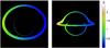 |
Fig. 1 Undeformed torus seen from an inclination of 45° (left) and 85° (right). The color bar, common to both panels, shows the ratio Δ ≡ (νobs/νem)3, where νobs and νem are the observed and emitted frequencies. This is the redshift factor that modulates the observed intensity. At high inclination, the beaming effect (which makes the redshift factor brighter on the approaching side of the torus) is more pronounced and the apparent area of the secondary image is bigger. |
At this stage, the deformed torus we are considering has thus only two degrees of freedom:
-
the torus thickness β parameter, with β ≪ 1,
-
the deformation parameter λ, with typically λ ≈ 1.
 |
Fig. 2 a) Normalized light curves for torus deformations. b) Normalized power spectral densities. Set of deformations with large maximal normalized values, |


3.2. Perturbed fluid 4-velocity
The fluid 4-velocity in the deformed torus is given by  (19)where
  is the equilibrium 4-velocity already defined in Eq. (2), which is assumed to be everywhere equal to its central value, in the slender torus limit.
The value of the perturbation δuμ induced by the deformation is easily computed by using the coordinate transformations given in the previous section. By writing a first-order expansion of  and
and  for a small time increment δt, it is straightforward to obtain the expressions of
  and
and  , which are themselves linearly related to dr/dt and dθ/dt.
An example of this is the case of radial translation of the torus cross-section:  (20)with
  (21)from Table 1.
As the torus is assumed to have a constant rescaled angular momentum ℓ0, the following relation holds between the non-equilibrium temporal and azimuthal covariant components of the 4-velocity:  (22)Adding the normalization condition uμuμ = − 1, Eqs. (20) to (22) fully determines the fluid 4-velocity. Equivalent formula can be derived for all other deformations.
4. Light curves and power spectra of the deformed torus
4.1. Ray tracing on the deformed torus
Light curves and power spectra of the deformed torus are computed by using the general relativistic ray-tracing code GYOTO (Vincent et al. 2011). Null geodesics are integrated backward in time from a distant observer’s screen to the optically thick torus. The zero of the surface function is found numerically along the integrated geodesic and the fluid 4-velocity is determined by using Eqs. (20). The specific intensity emitted by the undeformed torus is chosen to be constant throughout the surface. An image is then defined as a map of specific intensity.
Figure 1 shows the undeformed torus image as seen from an inclination of 45° and 85°. The two values of inclination emphasize the bigger impact of the beaming effect at high inclination, which strongly increases the dynamic of the image. Moreover, the apparent area of the primary and secondary images vary, depending on inclination. The primary image dominates clearly at small inclination, whereas the secondary image’s apparent area becomes important at high inclination. The value of β is chosen to ensure that the torus is indeed slender, i.e., that for all points inside the torus  (23)We choose β = 0.05, a value that satisfies these constraints well to be able to still abide by the slender torus approximation even for the deformed (and, in particular, extended) torus. This value will be fixed for the remainder of this article.
When the torus is deformed, two main effects will have an impact on the light curve: the change with time of projected emitting area and the varying amplitude of relativistic effects as the torus surface is approaching or receding from the black hole. To be able to compare the respective impacts of these two effects on the various deformed tori, we require that:
-
the specific intensity emitted at the surface of the optically thick torus is inversely proportional to its cross section. This will erase the effect of varying the flux by changing the torus cross-section area for torus expansion (all other deformations leave the cross-section area unchanged). Only the effect of changing the projected emitting area will thus remain;
-
the “closest approach” of the torus to the black hole, as defined by the minimum value of the r coordinate, is the same for all deformations. This ensures that the light emitted by the torus experiences comparable general relativistic effects, whatever the deformation. Precisely, we require that at closest approach,
 (compared with the initial minimum value of
  for the undeformed torus). We note that the
slender condition in Eq. (23) is
still satisfied.
for the undeformed torus). We note that the
slender condition in Eq. (23) is
still satisfied.
4.2. Light curves and power spectra
4.2.1. Definitions
Light curves are easily computed by calculating images of the deformed torus at various times. The time sampling was chosen to be around 100 frames per Keplerian period, and images are 1000 × 1000 pixels. As the Keplerian period at radius r0 = 10.8 M is tK = 230 M, the time interval between two frames is around δt = 2 M. The total number of frames computed for one given light curve is N = 200, thus covering around two Keplerian periods. One point on a light curve is simply equal to the summation of all pixels of a given frame (this boils down to summing intensity over all solid angles and thus to computing a flux).
Power spectral densities are computed in the following way. Let F(tk) be the flux value at time tk = kδt. The power spectral density at frequency fk = k/(Nδt) is defined as the square of the modulus of the fast Fourier transform of the signal, thus: 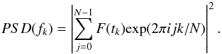 (24)
(24)
4.2.2. Observable characteristics of various deformations
Figure 2a) displays the light curves obtained for all deformations of the slender torus, seen with an inclination parameter of 5°, 45°, and 85°. The panels b) and c) of the same figure show the power density spectra of all deformations. The spectra are presented in two distinct panels for visibility as the power associated with different deformations or the same deformation at different inclinations varies significantly.
The biggest modulations (or biggest power densities) are obtained for deformations that lead to the biggest change of the torus apparent area. These deformations depend on inclination, but always include expansion and one or more shears.
The variation of relativistic effects linked to the changing torus location is less important than the change of apparent area. This is clearly demonstrated by noting that the smallest modulation is always obtained for vertical translation, which indeed leads to the smallest change of apparent area.
Whatever the inclination, expansion leads to a high power density, while translations and rotation give low power densities. On the other hand, shears exhibit a very inclination-dependent power density: radial and pure shears give high power for low inclination, while vertical shears give high power for high inclination. All these observable characteristics are directly linked to the change in apparent area of the deformed torus at various inclinations.
The time average of the light curves differs from one deformation to the other. It is dictated by the average value of the apparent area.
The dominating frequency of the light curves depends strongly on the deformation. Power is balanced between one time and two times the Keplerian frequency νK. Translations and expansion give a single-peak spectrum centered on νK. Rotation also gives a single-peak spectrum, but centered on 2 νK, as all possible values of apparent areas are covered after only half a Keplerian period in this case only. Shears give rise to a double-peak structure in the power spectrum, with a different balance of power between νK and 2 νK for radial, vertical, and pure shear.
4.3. Discussion
Figure 2 shows that the power spectral density is an interesting probe of the deformation of a slender accretion torus surrounding a black hole. Different kinds of deformations lead to significantly different power spectra.
It is interesting to note that the power density associated with expansion and the dominant shears is always one to two orders of magnitude higher than the power density associated with translations and rotation. This is due to the highly different evolution of the torus apparent area for these kinds of deformations.
The single- or double-peak nature of the power spectrum is also an interesting probe of the underlying kind of deformation. However, the very inclination-dependent aspect of the shears power spectra, as opposed to the other kind of deformations, presents a difficulty.
Taking these two probes into account (maximum power, dominating frequency) it is possible to constrain the kind of deformation by studying the power spectrum. Knowing the maximum value of power density, it is possible to determine whether the underlying deformation is within {expansion, shear} or {translation, rotation}. Then, as a function of the value of the dominating frequency, it is possible to determine the kind of deformation: expansion, shear, translation, or rotation. But it is not straightforward to determine what kind of translation or what kind of shear unless the inclination parameter is already constrained.
However, this work is only a first step towards a more sophisticated treatment of the observable characteristics of non-equilibrium accretion slender tori. Therefore, it is not the aim of this article to propose a way of constraining the motion of the accretion torus from the power density spectrum properties.
5. Conclusions and perspectives
We compute light curves and power density spectra of slender optically thick accretion tori surrounding a Schwarzschild black hole, which are subject to simple deformations (translations, rotation, expansion, and shears). We show that the power spectrum can be used to constrain the underlying kind of torus deformation.
This is a first step towards the full study of the observable characteristics of oscillating slender accretion tori. Our conviction is that combining simple deformations of slender tori will allow realistic oscillations to be mimicked. From this perspective, our present result that it is possible to differentiate various kinds of simple deformations from the observed power spectra is promising. Future work will determine whether this still applies when combinations of simple deformations are considered and whether this could lead to a practical tool for studying power spectra of high-frequency QPOs to constrain the underlying physical model. We believe that such tests can finally bring important outputs in the field of verifying the predictions of general relativity in the exploration of observational data accumulated so far. We also believe that outputs of sophisticated ray-tracing simulations could be key components of the proper interpretation of data received from planned future X-ray missions such as Large Observatory For X-ray Timing (Feroci et al. 2012).
Acknowledgments
We acknowledge support from the Polish NCN UMO-2011/01/B/ST9/05439 grant, the Swedish VR grant, and the Czech grant GAČR 209/12/P740. We further acknowledge the project CZ.1.07/2.3.00/20.0071 “Synergy” supporting the international collaboration of IF Opava. Computing was partly done using the Division Informatique de l’Observatoire (DIO) HPC facilities from Observatoire de Paris (http://dio.obspm.fr/Calcul/).
References
- Abramowicz, M. A., & Kluźniak, W. 2001, A&A, 374, L19 [NASA ADS] [CrossRef] [EDP Sciences] [Google Scholar]
- Abramowicz, M. A., Blaes, O. M., Horák, J., Kluzniak, W., & Rebusco, P. 2006, Classical Quant. Grav., 23, 1689 [Google Scholar]
- Blaes, O. M., Arras, P., & Fragile, P. C. 2006, MNRAS, 369, 1235 [NASA ADS] [CrossRef] [Google Scholar]
- Bursa, M., Abramowicz, M. A., Karas, V., & Kluźniak, W. 2004, ApJ, 617, L45 [NASA ADS] [CrossRef] [Google Scholar]
- Feroci, M., Stella, L., van der Klis, M., et al. 2012, Exp. Astron., 34, 415 [NASA ADS] [CrossRef] [Google Scholar]
- Fragile, P. C., Mathews, G. J., & Wilson, J. R. 2001, ApJ, 553, 955 [NASA ADS] [CrossRef] [Google Scholar]
- Karas, V. 1999, PASJ, 51, 317 [NASA ADS] [Google Scholar]
- Kato, S. 2001, PASJ, 53, 1 [NASA ADS] [CrossRef] [Google Scholar]
- Remillard, R. A., & McClintock, J. E. 2006, ARA&A, 44, 49 [NASA ADS] [CrossRef] [Google Scholar]
- Rezzolla, L., Yoshida, S., Maccarone, T. J., & Zanotti, O. 2003, MNRAS, 344, L37 [NASA ADS] [CrossRef] [Google Scholar]
- Schnittman, J. D., & Bertschinger, E. 2004, ApJ, 606, 1098 [NASA ADS] [CrossRef] [Google Scholar]
- Schnittman, J. D., & Rezzolla, L. 2006, ApJ, 637, L113 [NASA ADS] [CrossRef] [Google Scholar]
- Stella, L., & Vietri, M. 1999, Phys. Rev. Lett., 82, 17 [NASA ADS] [CrossRef] [Google Scholar]
- Stella, L., Vietri, M., & Morsink, S. M. 1999, ApJ, 524, L63 [NASA ADS] [CrossRef] [Google Scholar]
- Straub, O., & Šrámková, E. 2009, Class. Quant. Grav., 26, 055011 [Google Scholar]
- Tagger, M., & Varnière, P. 2006, ApJ, 652, 1457 [NASA ADS] [CrossRef] [Google Scholar]
- van der Klis, M. 2004 [arXiv:astro-ph/0410551] [Google Scholar]
- Vincent, F. H., Paumard, T., Gourgoulhon, E., & Perrin, G. 2011, Class. Quant. Grav., 28, 225011 [NASA ADS] [CrossRef] [Google Scholar]
- Vincent, F. H., Meheut, H., Varniere, P., & Paumard, T. 2013, A&A, 551, A54 [NASA ADS] [CrossRef] [EDP Sciences] [Google Scholar]
- Wagoner, R. V. 1999, Phys. Rep., 311, 259 [NASA ADS] [CrossRef] [Google Scholar]
All Tables
All Figures
|
Fig. 1 Undeformed torus seen from an inclination of 45° (left) and 85° (right). The color bar, common to both panels, shows the ratio Δ ≡ (νobs/νem)3, where νobs and νem are the observed and emitted frequencies. This is the redshift factor that modulates the observed intensity. At high inclination, the beaming effect (which makes the redshift factor brighter on the approaching side of the torus) is more pronounced and the apparent area of the secondary image is bigger. |
| In the text | |
|
Fig. 2 a) Normalized light curves for torus deformations. b) Normalized power spectral densities. Set of deformations with large maximal normalized values, |
| In the text | |
Current usage metrics show cumulative count of Article Views (full-text article views including HTML views, PDF and ePub downloads, according to the available data) and Abstracts Views on Vision4Press platform.
Data correspond to usage on the plateform after 2015. The current usage metrics is available 48-96 hours after online publication and is updated daily on week days.
Initial download of the metrics may take a while.