| Issue |
A&A
Volume 554, June 2013
|
|
|---|---|---|
| Article Number | A129 | |
| Number of page(s) | 6 | |
| Section | Stellar structure and evolution | |
| DOI | https://doi.org/10.1051/0004-6361/201321361 | |
| Published online | 17 June 2013 | |
Core collapse and horizontal-branch morphology in Galactic globular clusters
1
Department of Astronomy & Center for Galaxy Evolution
ResearchYonsei University,
120-749
Seoul,
Republic of Korea
e-mail:
This email address is being protected from spambots. You need JavaScript enabled to view it.
2
Yonsei University Observatory, 120-749
Seoul, Republic of
Korea
3
INAF–Osservatorio Astronomico di Teramo, Mentore Maggini s.n.c.,
64100
Teramo,
Italy
4
INAF–Osservatorio Astronomico di Roma, via Frascati 33,
00040
Monte Porzio Catone,
Italy
Received: 26 February 2013
Accepted: 3 May 2013
Abstract
Context. Stellar collision rates in globular clusters (GCs) do not appear to correlate with horizontal branch (HB) morphology, suggesting that dynamics does not play a role in the second-parameter problem. However, core densities and collision rates derived from surface-brightness may be significantly underestimated as the surface-brightness profile of GCs is not necessarily a good indicator of the dynamical state of GC cores. Core-collapse may go unnoticed if high central densities of dark remnants are present.
Aims. We test whether GC HB morphology data supports a dynamical contribution to the so-called second-parameter effect.
Methods. To remove first-parameter dependence we fitted the maximum effective temperature along the HB as a function of metallicity in a sample of 54 Milky Way GCs. We plotted the residuals to the fit as a function of second-parameter candidates, namely dynamical age and total luminosity. We considered dynamical age (i.e. the ratio between age and half-light relaxation time) among possible second-parameters. We used a set of direct N-body simulations, including ones with dark remnants to illustrate how core density peaks, due to core collapse, in a dynamical-age range similar to that in which blue HBs are overabundant with respect to the metallicity expectation, especially for low-concentration initial conditions.
Results. GC total luminosity shows nonlinear behavior compatible with the self-enrichment picture. However, the data are amenable to a different interpretation based on a dynamical origin of the second-parameter effect. Enhanced mass-stripping in the late red-giant-branch phase due to stellar interactions in collapsing cores is a viable candidate mechanism. In this picture, GCs with HBs bluer than expected based on metallicity are those undergoing core-collapse.
Key words: methods: statistical / methods: numerical / globular clusters: general / stars: evolution / stars: mass-loss
© ESO, 2013
1. Introduction
The color distribution of horizontal branch (HB) stars differs greatly among globular clusters (GCs; see, for example, Piotto et al. 2002). Since the 1950s, when metal abundances began to be determined for GCs, it was recognized that the first parameter responsible for this is metallicity (Sandage & Wallerstein 1960). However, it was also realized that it alone cannot fully account for the observed HB morphology, since observations showed that they can differ in the average position along the color coordinate in the HR diagram, in the overall extension, and in further additional features such as the presence of gaps. The task of singling out the mechanisms and the related observables that drive this diverse morphology, besides metallicity, is known as the second-parameter problem1. Over the years several candidate quantities have been claimed to be either the second parameter or a second parameter (see for a review Catelan 2009; Gratton et al. 2010). A (probably not exhaustive) list of these candidates are: age (Lee et al. 1994; Dotter et al. 2010), helium abundance (Lee et al. 2005; Busso et al. 2007; Piotto et al. 2007; Yoon et al. 2008), concentration (Fusi Pecci et al. 1993), binaries (Lei et al. 2013), and total GC mass (Recio-Blanco et al. 2006, R06 in the following). More recently, this long-standing issue attracted renewed interest after the discovery of multiple stellar populations in GCs (Bedin et al. 2004; Piotto et al. 2005, 2007; Busso et al. 2007; Yoon et al. 2008, among several others). However, a comprehensive picture is still lacking, and it is now clear that a single quantity is not capable of determining HB morphology in its whole complexity, so that more than one parameter is likely to play a role.
After the seminal work of Searle & Zinn (1978), the second parameter problem acquired a greater significance as a probe of the formation history of the Galaxy. Searle & Zinn (1978) pointed out that GCs with red HBs are usually found at galactocentric distances RGC > 8 kpc, while their occurrence is rare at smaller RGC. This led to the well-known inner halo-outer halo dichotomy, the outer halo GC population being accreted over an extended period of time according to the merging paradigm for galaxy formation. In this context, a quantity capable of explaining the differences in the mean temperature of the HB between inner- and outer-halo GCs in the Milky Way (MW) is often called a global second parameter. Amongst the various candidates, age is currently regarded as the most appropriate global second parameter (Lee et al. 1994; Dotter et al. 2010).
A quantity is instead termed as the local second parameter if it is capable of explaining the extension of the HB within a given GC. The discovery of multiple main sequences in GCs, together with the presence of extremely blue HB stars, has given strength to helium abundance as a local second parameter. A self-enrichment in helium and multiple generations of stars within an individual cluster can explain features such as tails and multimodalities in the HB (see D’Antona et al. 2002; Gratton et al. 2010; Joo & Lee 2013).
In this picture, dynamical processes (e.g. stellar encounters, binarity, stellar rotation) would not be involved in the global second-parameter issue, but their importance might be paramount as local second parameters, i.e. in connection to the extension of the HB (range of temperatures) rather than to its overall position in the HR diagram. After a GC forms, the negative heat capacity of the cluster self-gravity draws the cluster toward core collapse, unless another energy source is present. The central region or core will collapse to very large densities within a few relaxation times while the outer regions expand, and stars evaporate from the system. The standard energy source that is invoked to retard and to stop a further collapse is binaries (e.g. Goodman & Hut 1989). The contraction of the core via two-body relaxation increases its density. The core density determines the interaction rate in the core, which affects the single and binary star interaction probabilities at a given time. Core density is difficult to measure observationally because of the presence of invisible dark remnants. Moreover, the fraction of neutron stars and stellar-mass black holes that are expelled from GCs shortly after forming, due to natal-kick velocities, is poorly constrained. Due to this complexity in the evolution of dense star clusters, the only way to understand more about this picture is to perform numerical simulations including the physical processes mentioned above with a large number of stars of different types, i.e. visible stars and remnants.
The HB temperature distribution in Galactic GCs (GGCs) is usually interpreted as evidence of a dispersion in HB masses due to varying amounts of mass loss in the red-giant branch (RGB) phase. It is usually expected that the leading term in RGB mass-loss is due to stellar winds (Reimers 1977) and to reproduce the HB, an RGB mass-loss distribution is assumed accordingly, usually a Gaussian as first proposed by Rood (1973), and later used by Lee et al. (1994), Brocato et al. (2000), Raimondo et al. (2002). However, mass loss caused only by stellar wind is unable to explain the observed HB morphologies of some GCs in the MW (e.g., the hottest blue HB stars in NGC 2808, see Dalessandro et al. 2011). This points to another mass-loss process that may well be dynamical in origin, given that the physics of mass-loss is still poorly understood (e.g. Dupree et al. 2009). A numerical simulation study of RGB mass loss through encounters with white dwarfs and main sequence stars was performed by Davies et al. (1991) who characterized the dependence of mass-loss on the impact parameter and relative velocity of the encounter using a smoothed particle hydrodynamics (SPH) code. In this paper we report a finding that supports the view that mass-loss is related to the internal GC dynamics, in particular to core-collapse. We will investigate mass-loss through an encounter scenario in more detail in a future work (Moraghan et al., in prep.).
2. HB morphology and core density
R06 used Hubble Space Telescope photometry of a sample of 54 Milky Way GCs to determine the most probable second-parameter candidate for HB morphology, as quantified by the maximum effective temperature along the HB. In the present paper we introduce a new parameter, the cluster dynamical age, defined as the ratio between cluster age and half-light relaxation time and use the same data of R06 together with direct N-body simulations to investigate a possible correlation between HB morphology and GGC core density.
In general, different ways to quantify HB morphology may probe different physical processes and be subject to different statistical uncertainties and biases. While maximum effective temperature is an optimal indicator in the multivariate sense of the study by Babu et al. (2009), being based on an extreme value it is intrinsically noisier than central tendency estimates such as the mean and median. It is however more suitable to probe the physical processes that extend the HB towards high temperatures, which are more likely to be of dynamical origin as we argued above and show in the following. Dalessandro et al. (2012) found that maximum HB temperature from the R06 dataset correlates with ultraviolet colors obtained from GALEX integrated photometry, particularly with those involving far ultraviolet magnitudes. Therefore, even though maximum HB temperature based on optical colors, such as that of R06, might be underestimated in some cases (see Dalessandro et al. 2011, for example with NGC 2808), this quantity is still a useful parameter for characterizing HB morphology.
In their paper R06 compute the one-to-one linear correlation of the maximum effective temperature along the HB with metallicity, total GC luminosity, age, relaxation time, central density, and several other variables, and use the Principal Component Analysis (PCA; Pearson 1901) technique to check whether the best second-parameter may be a linear combination of a subset of these quantities. They find that the total luminosity is by far the most significant parameter in determining HB morphology after metallicity, and interpret this finding in terms of the GC self-pollution picture (D’Antona et al. 2002), where more massive (and therefore luminous) GCs managed to retain the helium-enriched ejecta of asymptotic giant branch stars. The authors conclude that linear correlations with central density, relaxation time, and the collisional parameter Γcol are marginally significant at best. This finding apparently rules out the role of stellar dynamics in the second-parameter problem.
In the next section, we show that the cluster dynamical age affects HB morphology in a nonlinear way: linear techniques such as PCA do not perform well when nonlinear associations between parameters are present (e.g. see Gorban & Zinovyev 2010), so this may be a reason why this effect was overlooked in R06, even though both parameters used to define dynamical age (chronological age and relaxation time) were considered separately.
The relation between maximum effective HB temperature and metallicity for the R06 GC sample is shown in Fig. 1, alongside an unweighted linear least-square fit (dashed straight line). We also applied local polynomial smoothing to extract the overall trend (solid and dash-dotted lines in Fig. 1) using the lowess() routine in the R programming language. This is a nonparametric technique where a polynomial is fit to the data inside a moving window, and makes use of an iterative re-weighing scheme to lower the influence of outliers, while recovering the trend from the data without the need for model assumptions. The dependence on metallicity is stronger for high-metallicity GCs. The slope decreases (and is even inverted) for low-metallicity GCs, while the scatter increases. However, as shown by the straight linear regression line, the overall slope is negative.
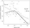 |
Fig. 1 Relation between maximum HB temperature and metallicity for R06 GCs. The superimposed straight dashed line is a linear least-square fit, and the solid line is a local polynomial regression smoothing. Three points appear visually as outliers to the relation: NGC 7078, NGC 6388, and NGC 6441. The dash-dotted line is the fit obtained without including them in the data-set. The difference with respect to the solid line is relatively small, due to the robust algorithm used for local polynomial regression (see text for details). |
2.1. Dependence on dynamical age
We define dynamical age as the ratio between chronological age and half-light relaxation time taken from Harris (1996). Absolute age is obtained from relative ages (Marín-Franch et al. 2009) normalized to 13 Gyr, where 5 clusters lacking a relative age measurement have been mean-substituted. In this section we quantify the effect of this parameter on maximum HB temperature.
In their analysis, R06 find that metallicity is the most influential parameter driving maximum HB temperature, based on linear measures of association (i.e. the correlation coefficient). In the following, we will therefore remove its effect by subtracting the temperature trend with metallicity before looking for a second parameter. It is however instructive to look directly at the relation between maximum HB temperature and dynamical age, uncorrected for metallicity, as shown in Fig. 2. It is clear that a global trend is present (as shown by the smooth solid line in Fig. 2), with an increase of the maximum HB temperature in the dynamical-age range of 5–10. However, the GCs in the highest-metallicity 25% of the sample (that also happen to have [Fe/H] ≥ −1.0; empty circles) follow a completely different trend (dashed line) and have on average lower HB temperatures. This is expected based on Fig. 1, as high-metallicity GCs show a very strong linear dependence of maximum HB temperature on metallicity. In the following we will therefore compare candidate second-parameters to the residuals to the temperature-metallicity relation instead of to temperature directly.
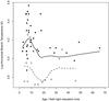 |
Fig. 2 Logarithm of maximum effective HB temperature as a function of dynamical age for the R06 sample, with superimposed local polynomial regression line (solid) showing the overall trend. High-metallicity GCs (the sample’s top 25% in metallicity, i.e. the GCs with [Fe/H] ≥ −1.0) are represented by empty circles, the rest by filled circles. Temperature peaks in the 5–10 relaxation-time range, but high metallicity GCs do not follow the trend. Their trend with dynamical age is shown by the dashed line. They are generally lower in HB temperature, because the main parameter affecting their HB temperature is metallicity, not dynamical age. |
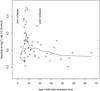 |
Fig. 3 Residuals to the local polynomial regression plotted in Fig. 1 (solid line in that figure) as a function of GC age to relaxation-time ratio. Core-collapse is found to occur for a ratio of about 5 to 10 depending on the mass spectrum and initial concentration (see simulations in the following). The superimposed local polynomial regression line (dashed) shows a peak in this age range. For comparison, the ticks on the vertical axis at the right side of the plot show (from bottom to top) the first quartile, the median, and the third quartile of the distribution of residuals. |
Figure 3 shows a plot of the residuals to the log T vs. [Fe/H] relation (obtained based on a local polynomial fit, as explained above) as a function of dynamical age. It turns out that clusters whose age is about 5 to 10 relaxation times have large residuals (i.e. bluer HBs than expected based on metallicity), while both dynamically-younger and older GCs have smaller residuals. A similar result is obtained if residuals to the linear fit to the log T vs. [Fe/H] relation are considered instead, as shown in Fig. 4. This is due to the fact that residuals to the linear fit and residuals to the polynomial fit are strongly correlated, with a linear correlation coefficient of 0.90.
Core density is expected to peak in the 5–10 relaxation times age range, due to core collapse (see discussion below). Several studies (e.g. see Buonanno et al. 1997; Testa et al. 2001) suggest that core density is a good candidate for the second-parameter role, but when the residuals are compared directly to the central density, R06 find no strong correlation. This may be due to the fact that central density estimates, such as those found in Harris (1996), are based on surface brightness profiles that are not good at tracing mass, especially in the central regions where heavy dark remnants such as neutron stars and stellar-mass black holes tend to segregate (Trenti et al. 2010). The same applies to expected rates of stellar collisions estimated from central velocity dispersions and central surface brightness, i.e. Γcol.
We run a set of direct N-body simulations using the N-body6 code (Aarseth 2010) in order to obtain the evolution of core density as a function of dynamical age. We then compare it with that of the residuals to the log T-[Fe/H] fit. Table 1 shows a summary of our simulations. They all contain a number of particles in the range 16 to 32 thousand, start from mass-unsegregated King-model initial conditions, and probe a range of discrete mass-spectra. Our models are isolated, i.e. no tidal forces from the galaxy have been included. The time at which core-collapse occurs, as well as its depth, is sensitive on the ingredients included in the simulation, such as the initial concentration and especially the binary fraction. However, the goal of the present paper is to show the presence of a pattern in GC data that can be interpreted in terms of core-collapse influencing HB morphology, so we do not probe the full simulation parameter space. In particular, our simulations start from low initial concentrations and have a primordial binary fraction of 02. While this is unrealistic, the goal of the simulations we present here is limited to illustrate how the temporal evolution of core density in GCs is remarkably similar to that of HB temperature (after removing metallicity dependence) without the need of a fine tuning of initial conditions.
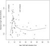 |
Fig. 4 Residuals to the linear regression plotted in Fig. 1 as a function of GC age to relaxation-time ratio (as in Fig. 3). The superimposed local polynomial regression line (dashed) is also obtained as in Fig. 3 and shows an overall very similar behavior of the residuals. |
In our analysis we define the core radius as the three-dimensional radius at which density drops by a factor 2 with respect to the central density. We then calculate the average mass-density within it. The simulations contain either three or four classes of stellar masses, and throughout our set we explore different number ratios between the classes. In all simulations the lightest class is the most abundant in number, in order to represent visible stars (luminous main sequence, RGB and HB). The heavier classes can be understood as invisible remnants, such as neutron stars and stellar-mass black holes, and different number ratios between the classes represent different retention fractions of dark remnants. Dynamical age is computed, for each simulation snapshot, by dividing its chronological age (in N-body units) by the half-mass relaxation time. We have adopted two different prescriptions for calculating the half-mass relaxation time: we either take the initial value of the half-mass relaxation time as obtained by N-body6 based on the initial conditions, or we recalculate it for each snapshot based on the actual half-mass radius and total mass of the model, according to the definition by Binney & Tremaine (1987). In the following we will refer to prescription (a) and (b) respectively. Since our models expand indefinitely (due to the lack of tidal limitation), half-mass radii tend to grow over time, producing an increasing half-mass relaxation time. In prescription (b) we first calculate the three-dimensional half mass radius rhall of all the particles, and then consider only those contained within three times rhall. While calculating the relaxation time self-consistently as in prescription (b) is more physically ground, there are, however, great uncertainties about relaxation times obtained from the observational data and on how to measure dynamical age in a consistent way both in simulations and observations (Djorgovski 1993; Harris 1996; McLaughlin & van der Marel 2005). Therefore we consider both prescriptions (a) and (b), and find that the differences are not dramatic, as we show in the following. Figure 5 compares the temporal evolution of core mass-density in direct N-body simulations with the residuals plotted in Fig. 3.
Summary of simulation runs in this paper.
Core density obtained from the simulations is shown as a function of dynamical age, i.e. the ratio between age and half-light relaxation time in the bottom panel of Fig. 5 (left, prescription (a); right, prescription (b)), while the top panel shows the residuals to the log T vs. [Fe/H] relation as in Fig. 3. The gray shaded area is the envelope of all the simulations in Table 1, and the black solid line is the global average. Core density, in all simulations in our set, peaks around 5–10 initial half-light relaxation times, when the self-similar collapse is halted by the formation of (at least) a binary due to three-body interactions. This is a general pattern that emerges in simulations of GCs irrespective of details related to the mass-function, so our choice of the mass-classes and number ratios discussed above does not change the qualitative evolution of density, even though a different mass spectrum will yield a quantitatively different evolution. However, it is clear from Fig. 5 that there is at least a qualitative similarity between the evolution of core density as a function of dynamical age and the residuals to the log T vs. [Fe/H] relation, and any further investigation of the details of the core-density evolution is beyond the scope of this paper.
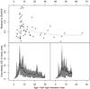 |
Fig. 5 Top panel: residuals to the metallicity fit associated to each GC, as in Fig. 3. Bottom panel, left: core mass-density in our set of direct N-body simulations of GCs (see Table 1) as a function of dynamical age. The gray shaded area is the envelope encompassing all simulations. The black solid line is the global average. The dynamical age was computed using the initial half-mass relaxation time (prescription (a) in the text). Bottom panel, right: same as left panel, but half-mass relaxation time was recomputed for each snapshot based on Binney & Tremaine (1987) definition (prescription (b) in the text). In both cases density peaks between 5 and 10 initial half-mass relaxation times. Upper and lower panels all share the same horizontal axis, but in the upper panel the abscissa values extend more, so we put axis labels on its upper side for improved readability. |
2.2. Dependence on luminosity
Figure 6 shows the residuals to the log T vs. [Fe/H] relationship (as obtained by local polynomial regression, see Fig. 1) as a function of the absolute magnitude MV. At about MV = −8, a threshold exists, and different behaviors are displayed by GCs above and below it. Low-luminosity clusters do not display any relation between luminosity and the residuals to the log T vs. [Fe/H] relationship, while high-luminosity ones do. A possible interpretation is based on the self-enrichment picture, where more massive clusters were able to retain more stellar ejecta, thus self-enriching more efficiently. However, current luminosity is not directly related to the original mass the cluster had at formation, as both the current mass-to-light ratio and the amount of mass lost during cluster lifetimes is uncertain (see Kruijssen & Portegies Zwart 2009, and references therein). It is anyway tempting to speculate that the magnitude threshold we observe in Fig. 6 corresponds to the minimum initial mass needed for self-enrichment to be efficient. Models of GC formation such as Recchi & Danziger (2005) predict a typical mass threshold for self enrichment that would correspond to an absolute magnitude MV of about −7.8, compatible with our analysis. Masses above the threshold would correspond to higher escape velocities, causing a better retention of chemically enriched gas. On the other hand, for any value of the mass below the threshold, enrichment would not occur, explaining why mass is no longer an influential variable and why the scatter becomes independent of magnitude.
Our analysis of the data is thus also compatible with the self-enrichment hypothesis, but as we have shown above this does not rule out a dynamical interpretation of the second-parameter effect. In other words, the data seem compatible with both scenarios.
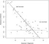 |
Fig. 6 Residuals to the local polynomial regression plotted in Fig. 1 as a function of GC absolute magnitude. Highly luminous clusters have larger residuals that increase with luminosity, while clusters less luminous than about −8 MV display no correlation between scatter and luminosity. If the current luminosity of a GC correlates with its initial mass, this pattern can be interpreted as an effect of self-enrichment, that was effective only for clusters above a given mass threshold. |
3. Comparison with other indicators of the GC dynamical state
The previous discussion can be summarized by stating that core collapse is a second-parameter of HB morphology, in the sense that GCs with bluer HBs (with respect to the metallicity prediction) are likely to be undergoing core-collapse. However, in Fig. 7 we show that there need not be visible signs of core collapse in the surface-brightness profile of a GC when it is in the dynamical age range of 5 to 10 half-light relaxation times. We plot the logarithmic core density of the R06 GCs from Harris (1996) as a function of dynamical age. The pattern that emerges shows a very mild peak at a dynamical age of about 15–20, as opposed to the stronger peak at 5–10 in Fig. 3. The density of visible stars probably correlates with the overall density, but with a large scatter. Sources of scatter are the shot noise from a limited number of bright stars, and differences in the present-day mass function and remnant abundance in different GCs, all contributing into making the surface-brightness profile a poor indicator of the dynamical status of the core.
Core-collapse is also often expected to produce a cusp in the surface-brightness profile of GCs, to the point that cuspy profiles are sometimes named collapsed-core GCs. There is a growing body of evidence, however, that the presence of a cusp in the surface brightness profile is neither sufficient nor necessary to conclude that the core is undergoing gravitational collapse. Trenti et al. (2010) use state-of-the-art direct N-body simulations to show that visible cusps may not form in GCs, resulting in light profiles that are well fit by a King model even during the core-collapse stage, if a realistic fraction of dark remnants (neutron stars and stellar-mass black holes) are included in the simulation. On the other hand, even if present, cusps are hard to detect without high angular resolution. In Fig. 7 filled circles represent clusters whose profiles are centrally cuspy. They are assigned a conventional value of the concentration parameter c = 2.5 in the Harris (1996) catalog. Except for having an overall higher value of core density, cuspy GCs do not have a clear pattern in the picture, again showing that the presence of a cusp is a poor proxy for dynamical age.
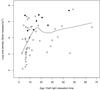 |
Fig. 7 Log core density of the R06 GCs (estimated from central surface brightness) as a function of dynamical age. Filled circles are high-concentration GCs which have been assigned c = 2.5 in Harris (1996). The surface-brightness profiles of these GCs show a central cusp, and they are often termed collapsed-core even though the link between cuspy profiles and dynamically collapsed cores is uncertain. Density estimated from surface brightness does actually show a mild peak at a dynamical age of about 15–20 (solid smoothing line), but does not follow a pattern as distinctive as that of the overall density obtained from simulations, and the presence of a central cusp is not a guarantee of old dynamical age. |
4. Conclusions and future prospects
We used data from R06 to show that internal dynamical processes can play a role in modeling the HB morphology in GGCs. In particular, GC dynamical age (chronological age measured in units of half-light relaxation time) affects HB morphology in a nonlinear way: GCs aged between 5 and 10 relaxation times have bluer HBs than expected based on the metallicity prediction alone, while dynamically younger and older GCs do not show large deviations. Since core-collapse is expected to take place in a similar range of dynamical ages, we suggest the presence of a link between the increased central density of collapsing cores and increased mass-loss in the RGB phase. However, core-collapse is not necessarily apparent from the GC surface-brightness profile, so the concentration parameter and/or the central surface-brightness are generally not good tracers of the GC dynamical state and will only marginally correlate with blue HBs.
Given that the R06 sample is quite representative of the GGC population, ranging from metallicities of −2.26 to −0.37 and absolute magnitudes from −5.56 to −9.82, we may infer from it that a relation between dynamical age and exceedingly blue HBs is present in the whole Galactic population, and possibly in extragalactic GCs too. By looking at Fig. 3 we see that about 20% of the R06 GCs have ages in the 5 to 10 half-light relaxation time range and exceedingly blue HBs (i.e. residuals to the metallicity fit in the top quartile), so over a population of about 200 GCs in the MW, we expect at least 40 where core-collapse has a visible effect on HB morphology.
How exactly core-collapse affects RGB mass-loss is still an open question. For example, Lei et al. (2013) propose the presence of a companion (i.e. the HB star being, or having been, part of a binary during its RGB evolutionary phase) as a candidate second-parameter. The companion would enhance mass-loss from the primary by tidal interaction, making the resulting HB star bluer. This theory is interesting in relation to our finding, as the number and binding energy of binaries in a
GC undergoing core collapse is expected to increase with time (Spitzer 1987). Core-collapse would then indirectly affect HB morphology by either creating binaries or reducing the separations of existing ones. Another possibility is that mass-stripping in the RGB phase is directly enhanced by stellar encounters, that are more frequent in a dense environment. We are currently modeling this process quantitatively using SPH simulations in order to provide a prediction of the mass-loss law at work in the high density environment of the core collapse GGCs.
Even though we retain this terminology for historical reasons, the implied assumption that a single second parameter can account for all the characteristics of the distribution of stars on the HB is unjustified in light of the current understanding of the issue.
However, binaries are formed dynamically at core collapse.
Acknowledgments
Support for this work was provided by the National Research Foundation of Korea to the Center for Galaxy Evolution Research, and also by the KASI-Yonsei Joint Research Program for the Frontiers of Astronomy and Space Science and the DRC program of Korea Research Council of Fundamental Science and Technology (FY 2012). This work received partial financial support by INAF−PRIN/2010 (PI G. Clementini) and INAF−PRIN/2011 (PI M. Marconi). We wish to thank the referee for comments and questions that helped us clarify several important points.
References
- Aarseth, S. J. 2010, Gravitational N-body Simulations (Cambridge, UK: Cambridge University Press) [Google Scholar]
- Babu, G. J., Chattopadhyay, T., Chattopadhyay, A. K., & Mondal, S. 2009, ApJ, 700, 1768 [NASA ADS] [CrossRef] [Google Scholar]
- Bedin, L. R., Piotto, G., Anderson, J., et al. 2004, ApJ, 605, L125 [NASA ADS] [CrossRef] [Google Scholar]
- Binney, J., & Tremaine, S. 1987, Galactic dynamics (Princeton, NJ: Princeton University Press) [Google Scholar]
- Brocato, E., Castellani, V., Poli, F. M., & Raimondo, G. 2000, A&AS, 146, 91 [NASA ADS] [CrossRef] [EDP Sciences] [Google Scholar]
- Buonanno, R., Corsi, C., Bellazzini, M., Ferraro, F. R., & Pecci, F. F. 1997, AJ, 113, 706 [NASA ADS] [CrossRef] [Google Scholar]
- Busso, G., Cassisi, S., Piotto, G., et al. 2007, A&A, 474, 105 [NASA ADS] [CrossRef] [EDP Sciences] [Google Scholar]
- Catelan, M. 2009, Ap&SS, 320, 261 [NASA ADS] [CrossRef] [Google Scholar]
- Dalessandro, E., Salaris, M., Ferraro, F. R., et al. 2011, MNRAS, 410, 694 [NASA ADS] [CrossRef] [Google Scholar]
- Dalessandro, E., Schiavon, R. P., Rood, R. T., et al. 2012, AJ, 144, 126 [NASA ADS] [CrossRef] [Google Scholar]
- D’Antona, F., Caloi, V., Montalbán, J., Ventura, P., & Gratton, R. 2002, A&A, 395, 69 [NASA ADS] [CrossRef] [EDP Sciences] [Google Scholar]
- Davies, M. B., Benz, W., & Hills, J. G. 1991, ApJ, 381, 449 [NASA ADS] [CrossRef] [Google Scholar]
- Djorgovski, S. 1993, in Structure and Dynamics of Globular Clusters, eds. S. G. Djorgovski, & G. Meylan, ASP Conf. Ser., 50, 373 [Google Scholar]
- Dotter, A., Sarajedini, A., Anderson, J., et al. 2010, ApJ, 708, 698 [NASA ADS] [CrossRef] [Google Scholar]
- Dupree, A. K., Smith, G. H., & Strader, J. 2009, AJ, 138, 1485 [NASA ADS] [CrossRef] [Google Scholar]
- Fusi Pecci, F., Ferraro, F. R., Bellazzini, M., et al. 1993, AJ, 105, 1145 [NASA ADS] [CrossRef] [Google Scholar]
- Goodman, J., & Hut, P. 1989, Nature, 339, 40 [NASA ADS] [CrossRef] [Google Scholar]
- Gorban, A. N., & Zinovyev, A. 2010, Int. J. Neural Syst., 20, 219 [CrossRef] [PubMed] [Google Scholar]
- Gratton, R. G., Carretta, E., Bragaglia, A., Lucatello, S., & D’Orazi, V. 2010, A&A, 517, A81 [NASA ADS] [CrossRef] [EDP Sciences] [Google Scholar]
- Harris, W. E. 1996, AJ, 112, 1487 [NASA ADS] [CrossRef] [Google Scholar]
- Joo, S.-J., & Lee, Y.-W. 2013, ApJ, 762, 36 [NASA ADS] [CrossRef] [Google Scholar]
- Kruijssen, J. M. D., & Portegies Zwart, S. F. 2009, ApJ, 698, L158 [NASA ADS] [CrossRef] [Google Scholar]
- Lee, Y.-W., Demarque, P., & Zinn, R. 1994, ApJ, 423, 248 [Google Scholar]
- Lee, Y.-W., Joo, S.-J., Han, S.-I., et al. 2005, ApJ, 621, L57 [NASA ADS] [CrossRef] [Google Scholar]
- Lei, Z.-X., Chen, X.-F., Zhang, F.-H., & Han, Z. 2013, A&A, 549, A145 [NASA ADS] [CrossRef] [EDP Sciences] [Google Scholar]
- Marín-Franch, A., Aparicio, A., Piotto, G., et al. 2009, ApJ, 694, 1498 [NASA ADS] [CrossRef] [Google Scholar]
- McLaughlin, D. E., & van der Marel, R. P. 2005, ApJS, 161, 304 [NASA ADS] [CrossRef] [Google Scholar]
- Pearson, K. 1901, Philosophical Magazine, 2 (11), 559 [Google Scholar]
- Piotto, G., King, I. R., Djorgovski, S. G., et al. 2002, A&A, 391, 945 [NASA ADS] [CrossRef] [EDP Sciences] [Google Scholar]
- Piotto, G., Villanova, S., Bedin, L. R., et al. 2005, ApJ, 621, 777 [NASA ADS] [CrossRef] [Google Scholar]
- Piotto, G., Bedin, L. R., Anderson, J., et al. 2007, ApJ, 661, L53 [NASA ADS] [CrossRef] [Google Scholar]
- Raimondo, G., Castellani, V., Cassisi, S., Brocato, E., & Piotto, G. 2002, ApJ, 569, 975 [NASA ADS] [CrossRef] [Google Scholar]
- Recchi, S., & Danziger, I. J. 2005, A&A, 436, 145 [NASA ADS] [CrossRef] [EDP Sciences] [Google Scholar]
- Recio-Blanco, A., Aparicio, A., Piotto, G., de Angeli, F., & Djorgovski, S. G. 2006, A&A, 452, 875 [NASA ADS] [CrossRef] [EDP Sciences] [Google Scholar]
- Reimers, D. 1977, A&A, 57, 395 [NASA ADS] [Google Scholar]
- Rood, R. T. 1973, ApJ, 184, 815 [NASA ADS] [CrossRef] [Google Scholar]
- Sandage, A., & Wallerstein, G. 1960, ApJ, 131, 598 [NASA ADS] [CrossRef] [Google Scholar]
- Searle, L., & Zinn, R. 1978, ApJ, 225, 357 [NASA ADS] [CrossRef] [Google Scholar]
- Spitzer, L. 1987, Dynamical evolution of globular clusters (Princeton, NJ: Princeton University Press) [Google Scholar]
- Testa, V., Corsi, C. E., Andreuzzi, G., et al. 2001, AJ, 121, 916 [NASA ADS] [CrossRef] [Google Scholar]
- Trenti, M., Vesperini, E., & Pasquato, M. 2010, ApJ, 708, 1598 [NASA ADS] [CrossRef] [Google Scholar]
- Yoon, S.-J., Joo, S.-J., Ree, C. H., et al. 2008, ApJ, 677, 1080 [NASA ADS] [CrossRef] [Google Scholar]
All Tables
All Figures
|
Fig. 1 Relation between maximum HB temperature and metallicity for R06 GCs. The superimposed straight dashed line is a linear least-square fit, and the solid line is a local polynomial regression smoothing. Three points appear visually as outliers to the relation: NGC 7078, NGC 6388, and NGC 6441. The dash-dotted line is the fit obtained without including them in the data-set. The difference with respect to the solid line is relatively small, due to the robust algorithm used for local polynomial regression (see text for details). |
| In the text | |
|
Fig. 2 Logarithm of maximum effective HB temperature as a function of dynamical age for the R06 sample, with superimposed local polynomial regression line (solid) showing the overall trend. High-metallicity GCs (the sample’s top 25% in metallicity, i.e. the GCs with [Fe/H] ≥ −1.0) are represented by empty circles, the rest by filled circles. Temperature peaks in the 5–10 relaxation-time range, but high metallicity GCs do not follow the trend. Their trend with dynamical age is shown by the dashed line. They are generally lower in HB temperature, because the main parameter affecting their HB temperature is metallicity, not dynamical age. |
| In the text | |
|
Fig. 3 Residuals to the local polynomial regression plotted in Fig. 1 (solid line in that figure) as a function of GC age to relaxation-time ratio. Core-collapse is found to occur for a ratio of about 5 to 10 depending on the mass spectrum and initial concentration (see simulations in the following). The superimposed local polynomial regression line (dashed) shows a peak in this age range. For comparison, the ticks on the vertical axis at the right side of the plot show (from bottom to top) the first quartile, the median, and the third quartile of the distribution of residuals. |
| In the text | |
|
Fig. 4 Residuals to the linear regression plotted in Fig. 1 as a function of GC age to relaxation-time ratio (as in Fig. 3). The superimposed local polynomial regression line (dashed) is also obtained as in Fig. 3 and shows an overall very similar behavior of the residuals. |
| In the text | |
|
Fig. 5 Top panel: residuals to the metallicity fit associated to each GC, as in Fig. 3. Bottom panel, left: core mass-density in our set of direct N-body simulations of GCs (see Table 1) as a function of dynamical age. The gray shaded area is the envelope encompassing all simulations. The black solid line is the global average. The dynamical age was computed using the initial half-mass relaxation time (prescription (a) in the text). Bottom panel, right: same as left panel, but half-mass relaxation time was recomputed for each snapshot based on Binney & Tremaine (1987) definition (prescription (b) in the text). In both cases density peaks between 5 and 10 initial half-mass relaxation times. Upper and lower panels all share the same horizontal axis, but in the upper panel the abscissa values extend more, so we put axis labels on its upper side for improved readability. |
| In the text | |
|
Fig. 6 Residuals to the local polynomial regression plotted in Fig. 1 as a function of GC absolute magnitude. Highly luminous clusters have larger residuals that increase with luminosity, while clusters less luminous than about −8 MV display no correlation between scatter and luminosity. If the current luminosity of a GC correlates with its initial mass, this pattern can be interpreted as an effect of self-enrichment, that was effective only for clusters above a given mass threshold. |
| In the text | |
|
Fig. 7 Log core density of the R06 GCs (estimated from central surface brightness) as a function of dynamical age. Filled circles are high-concentration GCs which have been assigned c = 2.5 in Harris (1996). The surface-brightness profiles of these GCs show a central cusp, and they are often termed collapsed-core even though the link between cuspy profiles and dynamically collapsed cores is uncertain. Density estimated from surface brightness does actually show a mild peak at a dynamical age of about 15–20 (solid smoothing line), but does not follow a pattern as distinctive as that of the overall density obtained from simulations, and the presence of a central cusp is not a guarantee of old dynamical age. |
| In the text | |
Current usage metrics show cumulative count of Article Views (full-text article views including HTML views, PDF and ePub downloads, according to the available data) and Abstracts Views on Vision4Press platform.
Data correspond to usage on the plateform after 2015. The current usage metrics is available 48-96 hours after online publication and is updated daily on week days.
Initial download of the metrics may take a while.