| Issue |
A&A
Volume 554, June 2013
|
|
|---|---|---|
| Article Number | A88 | |
| Number of page(s) | 12 | |
| Section | Astrophysical processes | |
| DOI | https://doi.org/10.1051/0004-6361/201321128 | |
| Published online | 07 June 2013 | |
Long term variability of Cygnus X-1
V. State definitions with all sky monitors
1
Dr. Karl−Remeis-Sternwarte and Erlangen Centre for Astroparticle Physics,
Friedrich Alexander Universität Erlangen-Nürnberg,
Sternwartstr. 7,
96049
Bamberg,
Germany
e-mail:
This email address is being protected from spambots. You need JavaScript enabled to view it.
2
Lawrence Livermore National Laboratory,
7000 East Ave., Livermore, CA
94550,
USA
3
CRESST, University of Maryland Baltimore County,
1000 Hilltop Circle,
Baltimore, MD
21250,
USA
4
NASA Goddard Space Flight Center, Astrophysics Science
Division, Code 661,
Greenbelt, MD
20771,
USA
5
Max-Planck-Institut für Radioastronomie,
Auf dem Hügel 69, 53121
Bonn,
Germany
6
MIT−CXC, NE80−6077, 77 Mass. Ave., Cambridge, MA
02139,
USA
7
Laboratoire AIM, UMR 7158, CEA/DSM − CNRS − Université Paris
Diderot, IRFU/SAp,
91191
Gif-sur-Yvette,
France
8
Space Sciences Laboratory, 7 Gauss Way, University of
California, Berkeley,
CA
94720-7450,
USA
9
European Space Astronomy Centre (ESA/ESAC), Science Operations
Department, PO Box 78, 28691
Villañueva de la Canãda, Madrid, Spain
10
Department of Physics, La Sierra University,
Riverside, CA
92515,
USA
11
Astronomical Institute “Anton Pannekoek”, University of
Amsterdam, Kruislaan
403, 1098 SJ
Amsterdam, The
Netherlands
12 Astrophysics, Cavendish Laboratory, University of
Cambridge, CB3 0HE, UK
13
Center for Astrophysics and Space Sciences, University of
California at San Diego, La Jolla,
9500
Gilman Drive, CA
92093-0424,
USA
14
ZP 12, NASA Marshall Space Flight Center,
Huntsville, AL
35812,
USA
Received: 18 January 2013
Accepted: 5 March 2013
Abstract
We present a scheme for determining the spectral state of the canonical black hole Cyg X-1 using data from previous and current X-ray all sky monitors (RXTE-ASM, Swift-BAT, MAXI, and Fermi-GBM). Determinations of the hard/intermediate and soft state agree to better than 10% between different monitors, facilitating the determination of the state and its context for any observation of the source, potentially over the lifetimes of different individual monitors. A separation of the hard and the intermediate states, which strongly differ in their spectral shape and short-term timing behavior, is only possible when data in the soft X-rays (<5 keV) are available. A statistical analysis of the states confirms the different activity patterns of the source (e.g., month- to year-long hard-state periods or phases during which numerous transitions occur). It also shows that the hard and soft states are stable, with the probability of Cyg X-1 remaining in a given state for at least one week to be larger than 85% in the hard state and larger than 75% in the soft state. Intermediate states are short lived, with a 50% probability that the source leaves the intermediate state within three days. Reliable detection of these potentially short-lived events is only possible with monitor data that have a time resolution better than 1 d.
Key words: X-rays: binaries / stars: individual: Cygnus X-1 / binaries: close
© ESO, 2013
1. Introduction
Accreting galactic black hole binaries (BHBs) show two main spectral states: a soft state with a thermal X-ray spectrum dominated by an accretion disk and a hard state with a power law spectrum with a photon index Γ ~ 1.7. The intermediate or transitional state can be subdivided into a hard-intermediate state and a soft-intermediate state (Belloni 2010). Transient BHBs also show a quiescent state (McClintock & Remillard 2006). All states show distinct spectral and timing properties in X-rays. Radio emission is detected in the hard and hard intermediate states and is strongly suppressed in the soft states (e.g., Fender et al. 2009).
In a hardness intensity diagram (HID) transient BHBs move on a clear trajectory, the so-called q-track (Fender et al. 2004). Different states correspond to different parts of the track. Of special interest is the so-called jet-line that roughly coincides with the transition from hard-intermediate to soft-intermediate state and is associated with radio ejection events (Fender et al. 2009). A q-track-like behavior on HIDs or on their generalization, the disk-fraction luminosity diagrams, has been found in different accreting sources such as neutron star X-ray binaries (e.g., Maitra & Bailyn 2004, Aql X-1), dwarf novae (Körding et al. 2008, SS Cyg), or active galactic nuclei (Körding et al. 2006). It is therefore likely to reflect basic accretion/ejection physics inherent to a wide range of accreting objects.
Cygnus X-1 is a key source for understanding accretion and ejection processes and their connection in BHBs. It is persistent, relatively nearby with a radio parallax distance of  kpc (Reid et al. 2011, consistent with X-ray dust scattering halo estimates of Xiang et al. 2011), and bright (above ~100 mCrab in the 1.5−12 keV band in the hard state), and it often undergoes (failed) state transitions (e.g., Pottschmidt et al. 2003), which are thought to be connected to changes in its radio jet (Fender et al. 2004, 2006; Wilms et al. 2007). The black hole is in a 5.6 d orbit around its donor star, HDE 226868 (Brocksopp et al. 1999b, and references therein). The orbital modulation is also detected in radio (e.g., Pooley et al. 1999) and due to modulation of the soft X-ray flux by absorption in the donor’s stellar wind in X-rays (Bałucińska-Church et al. 2000; Poutanen et al. 2008). Additionally, Cyg X-1 shows a superorbital period of 150 d (Brocksopp et al. 1999a; Benlloch et al. 2004; Poutanen et al. 2008), although that superorbital variability seems to be unstable and has recently been reported as having doubled to 300 d (Zdziarski et al. 2011a). In the hard state, radio jets have been observed (e.g., Stirling et al. 2001). The emisssion above ~400 keV Cyg X-1 is strongly polarized (Laurent et al. 2011; Jourdain et al. 2012).
As a persistent source Cyg X-1 does not cover the full q-track: its bolometric luminosity changes only by a factor of ~3−4 between the states (Wilms et al. 2006, and references therein) and its spectrum is never fully disk-dominated. The frequent state transitions (sometimes very fast − within hours, see, Böck et al. 2011) mean that the source often crosses the jet line. Since these state changes are thought to be associated with significant changes in the accretion flow geometry and energetics, a knowledge of the source state is crucial for interpreting all (multiwavelength) observations of Cyg X-1 and its donor star. A typical example is the study of the stellar wind of HDE 226868, which during soft states is strongly photoionized by the radiation from the vicinity of the black hole (Gies et al. 2008).
In the past decade, state information was readily available using the All Sky Monitor on the Rossi X-ray Timing Explorer (RXTE-ASM) and regular pointed monitoring observations. Here, various state definitions exist, which use, e.g., measured count rates and/or colors (e.g., Remillard 2005; Gies et al. 2008), or sophisticated mapping between these measurements and spectral parameters (e.g., Ibragimov et al. 2007; Zdziarski et al. 2011b). The former prescription is easy to use, but is very instrument-specific and cannot be translated easily to other X-ray all sky monitors. The latter approach requires a sophisticated knowledge of the instrumentation of all sky monitors, as well as of the detailed spectral modeling. Furthermore, the previously used state definitions are all slightly inconsistent among themselves. In this work we introduce a novel approach to classify states of Cyg X-1 using the all sky monitors RXTE-ASM, MAXI, Swift-BAT, and Fermi-GBM based on 16 years of pointed RXTE observations. Our aim is to find an easy-to-use prescription for determining the states that is as consistent as possible between these instruments in order to facilitate long-term studies that are longer than lifetime of individual monitors. We start with a description of our data reduction approach in Sect. 2. Section 3 comprises the actual state mapping from pointed RXTE observations to RXTE-ASM, Swift-BAT, MAXI, and Fermi-GBM, including a discussion of the precision of state determinations attainable with these instruments. We summarize and discuss our results in light of the statistics of the state behavior of Cyg X-1 in Sects. 4 and 5.
2. Observations and data analysis
2.1. ASM data
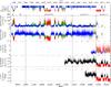 |
Fig. 1 Pointed RXTE observations and all light curves (RXTE-ASM, MAXI, Swift-BAT, and GBM) of Cyg X-1 used in this analysis. ASM, MAXI, and BAT data are shown in the highest available resolution, GBM are binned daily. ASM hardness is calculated by dividing count rates in band C (5.0−12 keV) by count rates in band A (1.5−3.0 keV). Vertical dashed lines and horizontal arrows represent periods of different source activity patterns. Blue, green, and red colors represent states of individual measurements classified using the respective classification for the different instruments as introduced in Sect. 3: blue represents the hard state, green the intermediate state and red the soft state. ASM data after MJD 55200 (shown in gray) are affected by intrumental decline. Hard and intermediate states cannot be separated in BAT and GBM; BAT and GBM data corresponding to these periods of hard or intermediate states are therefore shown in black. |
The RXTE-ASM instrument consisted of three Scanning Shadow Cameras (SSCs), in which a position sensitive proportional counter was illuminated through a slit mask (Levine et al. 1996). A typical source was observed at randomly distributed times five to ten times a day in three energy bands, roughly corresponding to 1.5−3.0 keV (band A), 3.0−5.0 keV (band B), and 5.0−12 keV (band C) (Levine et al. 1996).
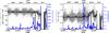 |
Fig. 2 Crab ASM light curve (left panel, 1.5−12 keV, gray points) and hardness (right panel, 5.0−12 keV/1.5−3.0 keV, gray points) with the respective 10-day average values (black histograms) and variances (blue histograms). |
We considered all 97556 RXTE All Sky Monitor (ASM, Levine et al. 1996) measurements of Cyg X-1 performed during the lifetime of RXTE. In the following all data analysis was performed with ISIS 1.6.2 (Houck & Denicola 2000; Houck 2002; Noble & Nowak 2008).
We first filtered for measurements where the background was clearly oversubtracted (count rates rA, rB, or rC < 0). The quality of the ASM data started deteriorating after about MJD 55200 (early January 2010): valid pointings are fewer and the overall variance of the measurements becomes larger (Fig. 1). Since the larger variance could be source intrinsic, we analyzed the ASM light curve of a source known to be roughly constant at the level of precision required here, the Crab (Wilson-Hodge et al. 2011): after MJD 55200 the Crab light curve shows prolonged gaps (Fig. 2). Where data exist, the average values of the ASM count rate (calculated on a 10 d timescale), which were stable at ~75 cps before, decrease by up to 10%. The variance of the data strongly increases by a factor of ~10. The ASM hardness (between the C and A bands) increases from stable values around ~0.95 to up to ~1.4 and shows higher variability. Both the timescale of this change in behavior and the similar behavior of the light curves of other sources during the same time period imply that we do not see the long-term variability of the Crab nebula as has been observed by Wilson-Hodge et al. (2011) here, but truly instrumental decline during the last years of the ASM lifetime1.
The ASM data measured post January 2010 can still be used to assess trends with large changes in count rate; however, for the following analysis, which relies on absolute values of both count rate and hardness, we ignore all ASM data after MJD 55200. Overall, we used 94 068 individual ASM measurements corresponding to 80 082 individual times (a source can be in the field of view of two SSCs simultaneously) spanning over 5000 days from MJD 50087 (1996 January 5) to MJD 55200 (2010 January 4).
2.2. Pointed RXTE observations
We consider all pointed RXTE observations of Cyg X-1 made during the RXTE lifetime (MJD 50071 to MJD 55931). Data from the proportional counter array (PCA, Jahoda et al. 2006) and the High-Energy X-Ray Timing Experiment (HEXTE, Rothschild et al. 1998) onboard RXTE were reduced with HEASOFT 6.11 following the procedure introduced in the previous papers of this series (Pottschmidt et al. 2003; Wilms et al. 2006).
For spectral analysis of the PCA data, we used data from the top xenon layer of proportional counter unit (PCU) 2. PCU 2 is the best calibrated PCU and had been running during all RXTE observations of Cyg X-1. We made use of the improved PCA background models and therefore only discarded data within ten minutes of the South Atlantic Anomaly (SAA; Fürst et al. 2009) passages, as opposed to the 30 min we used previously.
No HEXTE spectra were available during some observations either due to the nonstandard observation mode employed, mainly in early observations that are not part of our bi-weekly campaign, or due to the failure of the rocking mechanism of the HEXTE clusters in the last years of the RXTE lifetime.
We extracted all PCA spectra in the standard2f mode for each RXTE orbit and obtained 2741 individual spectra. The improved PCA background and response allowed us to consider a wider energy range than previously, namely ~2.8 keV to 50 keV. The wider overlap between the PCA and HEXTE spectra, which are considered between 18 keV and 250 keV, leads to a better constraint on the multiplicative constant that accounts for the differences in the flux calibration of the two instruments. Following Böck et al. (2011) and Hanke (2011), we added a systematic error of 1% to the fourth PCA bin (2.8−3.2 keV) and of 0.5% to the fifth PCA bin (3.2−3.6 keV) in the data from PCA’s calibration epoch 5 (2000 May 13−2012 January 5)2, which constitute the majority of our dataset. For epochs one to four we aimed for the closest possible match in energy for the systematic errors.
Where possible due to the available PCA modes, light curves with a time resolution of 2-9 s (~2 ms) were extracted for timing analysis, choosing the same energy bands as Böck et al. (2011): a low-energy band corresponding to energies 4.5−5.7 keV (channels 11−13) and a high-energy band corresponding to energies 9.4−14.8 keV (channels 23−35; energy conversion for epoch 5). Calculation of the rms and X-ray time lags follows Nowak et al. (1999). We used segments of 4096 bins; i.e., we calculated the root mean square variability (rms) between 0.125 and 256 Hz.
For two simultaneous, correlated light curves, such as the high- and low-energy light curves of Cyg X-1 used here, one can calculate a Fourier frequency dependent time lag between the two from the Fourier phase lag at any given frequency (Nowak et al. 1999, and references therein). In our calculations a positive time lag means that the light curve in the hard energy band is lagging the soft. The timelag depends strongly on Fourier-frequency and shows a complex variation with state see (see Pottschmidt et al.2000 for examples and note that we use the same frequency binning in the relevant frequency range). To obtain a single value that serves as a good signature for the overall level of the lags, we average it over the frequency range of 3.2−10 Hz (see Pottschmidt et al. 2000, 2003).
2.3. Swift-BAT, MAXI, and Fermi-GBM data
RXTE was switched off on 2012 January 5 (MJD 55931). To continue the monitoring of the long term behavior of Cyg X-1 we therefore need to use other instruments. The all sky monitor available in the soft X-ray band at the time of writing is MAXI, the hard X-rays above 10 keV are covered by Swift-BAT and Fermi-GBM.
MAXI is an all-sky monitor onboard the Japanese module of the International Space Station (Matsuoka et al. 2009). Light curves from the Gas Slit Camera detector (GSC) are available in three energy bands (2−4 keV, 4−10 keV and 10−20 keV) on a dedicated website3. MAXI light curves show prolonged gaps of several days due to observational constraints.
Swift-BAT is sensitive in the 15−150 keV regime (Barthelmy et al. 2005). Satellite-orbit averaged light curves in the 15−50 keV energy band from this coded mask instrument are available on a dedicated website4.
The Gamma-ray Burst Monitor (GBM; von Kienlin et al. 2004; Meegan et al. 2007) onboard Fermi observes the sky in the hard X-ray and soft γ-ray regimes (about 8 keV to ~30 MeV). It permanently provides complete coverage of the unocculted sky. Because of its strongly limited spatial resolution, the brightness of individual sources cannot be determined directly and so the Earth occultation method is applied (Case et al. 2011; Wilson-Hodge et al. 2012). In this work we use the publicly available quick-look Fermi GBM Earth occultation results provided by the Fermi GBM Earth occultation Guest Investigation teams at NASA/MSFC and LSU5, which consist of light curves with a 1 d resolution in four energy bands between 12 keV and 300 keV (12−25 keV, 25−50 keV, 50−100 keV, and 100−300 keV) starting from MJD 54 690. On average each measurement of Cyg X-1 is based on 18 occultations.
As these data are prescreened by the respective instrument teams, no further selection criteria were applied, and we used all data available from the start of the each mission until MJD 56240, resulting in 36 454 individual measurements for BAT, 9794 for MAXI, and 1443 for GBM (Fig. 1).
3. Identifying the states of Cygnus X-1
3.1. General source behavior
The different periods of source activity and therefore the different population of the individual source states strongly affect our ability to distinguish the regions that the respective states occupy on HIDs or in other spaces. As a first step for our analysis we therefore present an overview of the light curves used for this work and over the ASM 5−12 keV to 1.5−3 keV hardness (Fig. 1).
The source behavior from early 1996 (RXTE launch) until the end of 2004 has been discussed by Wilms et al. (2006), who used a crude definition of ASM based states using only the count rate. This classification is sufficient to distinguish main activity patterns, and also consistent with more detailed studies (Zdziarski et al. 2011b). We extend this earlier work and supplement the ASM data with BAT, MAXI, and GBM. By eye, i.e., without using the state definitions introduced later in this section and shown in color in Fig. 1, we are able to distinguish five main periods with different source activity patterns:
-
a pronounced soft-state episode in 1996 (up to ~MJD 50350, period i);
-
one and a half years of a mainly stable hard state with only short softenings, seen as spiky features in Fig. 1, between the end of 1996 and early 1998 (~MJD 50350−51 000, period ii);
-
a series of failed state transitions and soft states that started in early 1998 (Pottschmidt et al. 2003) and included a prolonged, very soft period between the end of 2001 and the end of 2002. This activity period continued until mid-2006 (~MJD 51 000−53900, period iii);
-
an almost continuous hard state from mid-2006 to mid-2010, which includes the hardest spectral states ever observed in Cyg X-1 (see Nowak et al. 2011, ~MJD 53900−55375, period iv);
-
a series of prolonged soft states that followed an abrupt state transition at ~MJD 55375 and continued during the writing of this paper (>MJD 55375, period v).
Periods i to iii are fully, and period iv is almost fully covered by the ASM. Some ASM data exist during period v, but are affected by problems described in Sect. 2.1 and therefore excluded from our analysis. During period iv the ASM hardness shows higher variability than in previous hard states, but the same effect is also seen in the hardness of the Crab and is instrumental (Fig. 2).
BAT coverage started at the end of period iii on MJD 53414 (mid-February 2005) and continues during the writing of this paper. Thus, BAT data are available during soft states, namely in period v, but simultaneous coverage of soft states by BAT and ASM is lacking.
GBM and MAXI coverage started MJD 54 690 (2008 August 12) and MJD 55058 (2009 August 15), respectively, and was going on when this paper was written. These instruments mainly cover the final phase of period iv and the ongoing period v. No simultaneous coverage with ASM exists during the intermediate and soft states, except during the phase of ASM deterioration.
During the joint coverage by ASM and BAT, Cyg X-1 displayed two softening episodes, which did not reach a stable soft state (~MJD 53800−53900 and around MJD 55000). Both episodes are clearly visible in the ASM band but not in the BAT light curve. This is a remarkable contrast to the full state transition of ~MJD 55375, which is associated with a clear drop in the BAT count rate simultaneous with an increase in the ASM count rate. Similar softenings visible in the soft X-ray band but not in the hard band have been observed in 1997−1999 by Zdziarski et al. (2002), who discuss changes seen in the ASM where no corresponding changes were observed in the 20−300 keV band with BATSE. Only further long-term observations in both soft and hard X-rays can help decide whether only successful state transitions are accompanied by a change in hard X-ray flux and whether the behavior of the hard component above 15−20 keV can be used to decide whether a state transition will fail or not.
Reliable ASM data are lacking after MJD 55200. The BAT light curve suggests that while the source left the soft state for short periods of time, those hard periods were softer than the prolonged hard states in periods ii and iv.
A striking feature of the hardness during the hard states are values that exceed the average by a factor of ~5 and more (Bałucińska-Church et al. 2000; Poutanen et al. 2008). They correspond to so-called X-ray dips, where blobs of cold material in the line of sight cover the source. Since it is virtually impossible to decide whether an individual ASM dwell was measured during a dip, we do not treat these data separately for the purpose of this paper (but see Boroson & Vrtilek 2010).
3.2. Γ1-defined states
Wilms et al. (2006) have shown that the spectral shape of Cyg X-1 as observed by PCA and HEXTE (from here on: RXTE spectrum) can be described well by an empirical model that consists of a broken power law modified by a high-energy cut-off and absorption described by the tbnew model, see, e.g., Hanke et al. (2009), and the abundances of Wilms et al. (2000). The iron Kα line is described by an additive Gaussian emission line at ~6.4 keV. The intermediate and soft states additionally show a soft excess, which is usually described by accretion disk emission (Mitsuda et al. 1984; Makishima et al. 1986). The soft photon index, Γ1, of the broken power law shows strong correlations with other spectral and timing parameters on timescales from hours to years across the whole range of its values and is a good proxy for the source state (e.g., Pottschmidt et al. 2003; Wilms et al. 2006; Böck et al. 2011; Nowak et al. 2011).
We model all spectra both with and without a disk and accept the disk as real if the addition of the disk component improves the χ2 value by more than 5%6. With this approach, we are able to achieve good fits ( ) for almost all spectra, with a few outliers not exceeding
  . Fewer than 18% of the spectra with Γ1 < 2.0 require a disk, but 97% of the fits with Γ1 > 2.0 do. This agrees with the known behavior of the disk in BHBs in the different states (e.g., Belloni 2010). For all best fit models, we obtain Γ1 > Γ2 and Ebreak ~ 10 keV. For a more detailed discussion of the fits to then available data and examples of typical spectra we refer to Wilms et al. (2006).
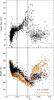 |
Fig. 3 X-ray time lag and fractional rms as a function of the soft photon index Γ1. |
Figure 3 shows the dependence of the total rms between 0.125 and 256 Hz in both-high and low-energy bands and the time lag (averaged between 3.2 and 10 Hz) on the soft photon index Γ1. The timing and spectral behavior is clearly related, but is complex with changes in both slope and sign. For clarity in the plot we do not show error bars; however, the uncertainity of single measurements is close to or smaller (much smaller in the case of the hard observations) than the spread of the correlation at any given frequency. The value of Γ1 ~ 2, where spectral models with a disk become dominant, corresponds to a bend in the timing correlations. Another clear kink can be seen at Γ1 ~ 2.5.
We use both our spectral and timing analysis results to define Γ1 ranges for different source states that are characterized by spectral and timing behavior that is similar within a state but different between the three states. Hard states correspond to Γ1 < 2.0, intermediate states correspond to 2.0 < Γ1 < 2.5, and soft states correspond to Γ1 > 2.5.
3.3. Simultaneous ASM mapping
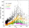 |
Fig. 4 Dependence of the ASM count rate in different bands on the soft photon index Γ1 of simultaneous pointed RXTE observations. Shown are total ASM counts (1.5−12 keV, black dots) and counts in the three ASM energy bands: band A (1.5−3 keV, orange upside down triangles), band B (3−5 keV, green triangles), and band C (5−12 keV, magenta squares). |
For direct classification of the ASM data, we use the 1424 instances when ASM observations of Cyg X-1 are simultaneous with spectra from pointed RXTE observations, i.e., fall within the good time intervals used for the orbit-wise spectral extractions. This corresponds to 2400 individual ASM measurements since the source is often observed by more than one SSC. We treat the measurements of different SSCs independently for the actual mapping since instrument alignment onboard RXTE would otherwise introduce a bias towards a higher number of ASM measurements with Cyg X-1 in the field of view of two SSCs during pointed observations of Cyg X-1.
Spearman’s rank correlation coefficients ρ between the ASM counts and the soft photon index Γ1
Figure 4 shows the dependence of the ASM count rate from individual ASM-SSC dwells on the soft photon index Γ1 of the broken power law fits. Because of the use of individual ASM SSC dwells, an RXTE spectrum, hence a Γ1-value, can correspond to more than one simultaneous ASM measurement. While the ASM count rate in all bands is correlated with Γ1, this correlation is not unique: it appears to change sign at Γ1 ~ 2.7 (Table 1). Consistent with this observation, Zdziarski et al. (2011b) note that on several instances in the soft state their derived bolometric flux is lower than during the high-flux hard state7. Thus, cuts in ASM count rate alone cannot separate the states.
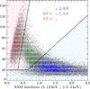 |
Fig. 5 PCA to ASM mapping. Gray data points are all ASM measurements of Cyg X-1 in the shown range. Blue points represent PCA defined hard states, green intermediate and red soft states. Black lines show the cuts defining the states in the ASM HID. The light blue shaded region corresponds to the position of the hard state in the HID, the light red shaded to the position of the soft state. The intermediate state region is shown without shading. |
Overview over all sky monitor based state definitions for Cyg X-1.
The Γ1-based definition of states introduced in Sect. 3.2 results in in 1608 ASM measurements in the Γ1-defined hard state, in 455 ASM measurements in the Γ1-defined intermediate state, and in 337 ASM measurements in the Γ1-defined soft state. Each of the states primarily populates a well-defined distinct area in the ASM HID (Fig. 5). A visual inspection reveals that neither cuts in hardness alone nor cuts in count rate alone yield a good division between the states. The softest observations tend to have count rates in the transitional state range (~40−50 cps), the hard state area extends to low hardnesses usually associated with transitional or even soft states, and the hard and transitional states strongly overlap both in ASM hardness and count rate. To account for these features, we choose the following ansatz: an ASM observation with count rate c and (5−12 keV/1.5−3 keV) hardness h is defined as hard if c ≦ 20 cps regardless of the hardness. For c > 20 cps the cuts between the states are defined by linear functions of the form 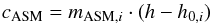 (1)where i ∈ {hard,soft}. The line with slope mASM,hard and x-intersection h0,hard divides the hard and the intermediate states, and the line with slope msoft and intersection h0,soft divides the intermediate and the soft states, respectively.
We determine the best division between the states such that the fractional contamination of the ASM-defined states by different Γ1-defined states is minimized. Contamination here is defined for the hard state (and accordingly for soft and transitional states) as the fraction of all measurements classified as hard using the ASM that is classified as transitional or soft according to Γ1. Initial fits indicate that good separations of the states are achieved for h0,hard ~ h0,soft. We therefore reduce the number of free parameters for the cuts and set 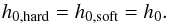 (2)For the best cuts we obtain h0 = 0.28, mhard = 55, and msoft = 350 (Fig. 5 and Table 2).
The contamination by other Γ1-defined states is <5% for the hard state, <10% for the intermediate state and <3% for the soft state. Note that since the source behavior changes continuously from one state to the other, such that the states do not represent three distinct, fully independent regimes, we do not expect a perfect separation of the states (e.g., Wilms et al. 2006). The spread in count rate and hardness is amplified by the orbital and superorbital modulations of Cyg X-1 and by dips (e.g., Poutanen et al. 2008). The stronger contamination of the intermediate state is expected: as a transitional state between the hard and the soft state, it is short-lived and confined by two divisional lines. The separation between the hard and the intermediate state appears especially unclean; we therefore advise to treat the classification cautiously when an observation is close to this cut.
To test our approach we compare the ASM-based behavior with the results of the spectro-timing analysis of the quick, observationally exceptionally well covered intermediate to soft transition presented by Böck et al. (2011). In particular, we can recover the moment of the transitions at slightly before MJD 53410.
3.4. Non-simultaneous ASM mapping
In general, an all sky monitor and a pointed instrument will not observe a source at the same time, so that we need to assess how well a given monitor pointing can be used to characterize the source state during a non-simultaneous observation. For every RXTE spectrum we consider ASM measurements within 1.5 h intervals Δt = ± (0–1.5) h, ± (1.5–3) h, ± (3–4.5) h, etc., up to 48 hours. The length of the intervals is motivated by the length of the RXTE orbit of ~1.5 h, during about half of which Cyg X-1 is visible. For simultaneous ASM measurements with different SSCs we use the average for all subsequent analysis. We obtain 135 901 pairs of ASM and RXTE state classifications (the same ASM measurement may be used to classify several RXTE spectra, if the RXTE spectra are close enough). For each delay interval and for each ASM defined state, we determine the percentage of spectra with a different RXTE classification.
Figure 6 shows that this contamination remains stable for the hard state for up to ~48 h. For the soft state, the contamination reaches 20% for a 48 h delay and is even greater for the intermediate state, which also shows a very strong increase within the first ~10 h. Strictly simultaneous data, which were discussed in Sect. 3.3, are not taken into account here, resulting in higher starting contaminations. The results are similar when using positive or negative delays only. The trends are expected, because the hard state often occurred in long, stable stretches during the RXTE lifetime, while the intermediate state is short lived due to its transitional nature.
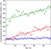 |
Fig. 6 Percentage of contamination of the ASM defined states (hard state shown in blue, intermediate in green, and soft in red) for time delays Δt = ± (0–1.5) h, ± (1.5–3) h, ± (3–4.5) h, etc., between the ASM and the pointed RXTE measurements. Simple linear fits to the data are shown as dashed lines to illustrate the overall trends. |
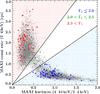 |
Fig. 7 PCA to MAXI mapping. Gray data points are all MAXI orbitwise measurements of Cyg X-1 in the shown energy range. Blue circles represent Γ1-defined hard states, green intermediate states and red soft states. Black lines define the state cuts. The light blue shaded region corresponds to the hard state in the MAXI HID, the light red shaded region to the soft state, and the region without shading to the intermediate state. |
3.5. MAXI mapping
Since only 37 MAXI measurements are strictly simultaneous with pointed RXTE data, we use MAXI data within Δt = 1 h before and after a pointed RXTE observation and obtain 219 MAXI measurements with Γ1-based state classifications, which offer a better overall statistics with 107 hard states, 101 soft states, and 11 intermediate states. Increasing Δt to 2 h does not yield a better coverage of the intermediate state, neither does attempting to map ASM onto MAXI, since a simultaneous coverage by the two instruments is only available during the end of period iv.
To find the best approach for defining MAXI-based states, we considered all possible different combinations of count rates measured with MAXI (the three energy bands as introduced in Sect. 2.3 and the overall count rate) and different combinations of hardness measures within the MAXI bands. The clearest separation can be achieved when using the ratio between count rates in the medium (4−10 keV) and the low (2−4 keV) MAXI bands (MAXI-hardness, hMAXI) and the count rate in the low (2−4 keV) MAXI band, cMAXI, as done in Fig. 7. The MAXI 4−10 keV/2−4 keV hardness is also the closest correspondence to ASM hardness we can achieve using publicly available MAXI light curves.
The sparse coverage of the intermediate state makes it hard to separate the three basic states. Given that the hard and the soft states populate distinct parts of the MAXI HID (see Fig. 7) and knowing the shape of the cuts in the ASM HID, we separate the states by two linear functions of the form 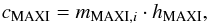 (3)where i ∈ {hard,soft}, mhard separates the hard and the intermediate states and msoft separates the intermediate and the soft states. The absence of an x-intersection and of a threshold count rate value is motivated by the lower number of classified data points compared to the ASM HID, which also prevents us from direct fits for m. The best values obtained by eye are mMAXI,hard = 1.4 and mMAXI,soft = 8/3 (Table 2).
For a reader interested in performing her own classification using MAXI data, we note that these are conservative cuts in the sense that we obtain the purest intermediate state possible here. As in the case of RXTE-ASM we expect the separation between the hard and intermediate states to be especially unclean.
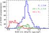 |
Fig. 8 Histogram of BAT fluxes of Γ1-defined states. The hard state is shown in blue, the intermediate state in green, and the soft state in red. |
3.6. BAT mapping
Swift-BAT light curves in different energy bands are not readily available. Since BAT also does not cover soft X-ray energies where the contribution of the accretion disk becomes important as the spectrum softens, we use only the light curves in the standard 15−50 keV band for our analysis and therefore do not perform a two-dimensional mapping.
Since only 290 BAT measurements are strictly simultaneous with pointed RXTE data, we employ the same approach as for MAXI (Sect. 3.5) and use BAT data within Δt = 1 h before and after the RXTE spectrum to obtain 1339 BAT measurements with an RXTE based state classification: 895 in the hard state, 124 in the intermediate state, and 320 in the soft state.
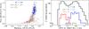 |
Fig. 9 Left: daily GBM HID. S denotes the 12−25 keV flux, H the 25−50 keV flux. The gray dashed line denotes the zero flux level. Total GBM measurements are shown in gray. Right: histogram of daily GBM fluxes of Γ1-defined states. The hard state is shown in blue, intermediate state in green, and soft state in red. Total GBM measurement are shown in black. The gray dashed line denotes the zero flux level. |
Only 290 BAT measurements are strictly simultaneous with pointed RXTE data. Following our study of the reliability of nonsimultaneous data (Sect. 3.4), we used BAT data within Δt = 1 h before and after a pointed RXTE observation, and obtain 1339 BAT measurements with Γ1-based state classifications, which offer better overall statistics.
Figure 8 shows the histogram of the BAT fluxes in the different states. While the soft and hard state clearly show different BAT fluxes, the intermediate states populate the same region as the hard ones. The BAT measurements, therefore, do not enable us to separate the hard and the intermediate states. The soft state can still be identified by a cut at a BAT area-normalized count rate of cBAT = 0.09 counts cm-2 s-1 For BAT count rates below cBAT, Cyg X-1 is in the soft state, for fluxes above it in the hard or intermediate states (Table 2). The contamination by the other state is ~7% in both cases.
We also considered an ASM to BAT mapping where we classified BAT data by using the closest ASM measurements if one exists within ±0.5 h around the BAT measurement in order to increase the number of data points with classification. No simultaneous good ASM and BAT data are available in the soft state (see Fig. 1 and Sect. 2.1). The histograms of the hard and intermediate states follow the trends apparent from Fig. 8: it is not possible to separate the two states using BAT flux.
3.7. GBM mapping
Since GBM light curves are publicly available only in daily bins, strictly simultaneous mapping between RXTE spectra and GBM is not possible. We therefore define an RXTE spectrum as simultaneous to a GBM measurement if the good time interval used to extract the spectrum lies within the GBM measurement. If all simultaneous RXTE spectra show the same state, the GBM measurement is classified as belonging to this state. If the states of the RXTE spectra differ, the GBM measurement is not classified.
The 104 GBM measurements with simultaneous RXTE observations include on average 3.8 (reaching from 1 to 8) individual RXTE spectra. Only 6 out of the 104 measurements are unclassified due to state ambiguities. The remaining valid classifications include 61 hard states, 3 intermediate states, and 34 soft states. All 6 unclassified measurements include hard and intermediate state classifications. There were no GBM measurements including both intermediate and soft, or hard and soft RXTE spectra. The distribution of these results is consistent with Cyg X-1 spending most of the time covered by GBM observations in stable hard and soft states. That six out of nine GBM measurements including a Γ1-defined intermediate state also include Γ1-defined hard states reflects the high variability and instability of the intermediate states.
We first consider GBM HIDs. These show a clear separation in two regions: a region with mainly soft and a region with hard and intermediate observations, which are clearly separated in GBM flux alone. We therefore consider only GBM fluxes and calculate histograms of GBM fluxes of Γ1-defined states. The best separation between the states can be achieved when using 25−50 keV fluxes (Fig. 9). While hard and intermediate states cannot be separated, the soft state can be divided from the other two by a cut at a GBM flux of 0.6 Crab: for fluxes <0.6 Crab the source is in the soft state, for fluxes ≥0.6 Crab in hard or intermediate state (Table 2). We do not give values for contamination here because of the long integration times of the GBM and because we excluded states where we know the source to change the Γ1 defined state during one GBM measurement. We also note that since the hard and intermediate states cannot be distinguished using GBM, we did not introduce additional bias into our classification by not including GBM-measurements with simultaneous RXTE spectra in both hard and intermediate states.
Time Cyg X-1 spent in the different states (hard − H, intermediate − I, soft − S) as measured by the RXTE-ASM, Swift-BAT, MAXI, and Fermi-GBM all sky monitors.
4. The states of Cyg X-1
4.1. The statistics of Cyg X-1 states
Using the classification from the different instruments derived in the previous sections, we can assess the activity pattern during the different periods defined in Sect. 3.1. A detailed breakdown of the occurrence of different states is given in Table 3.
Period i contained a prolonged soft state, and the source spent twice as much time in soft state as in the intermediate state during this time. We lack all sky monitor coverage before MJD 50087, and therefore do not know whether this soft period observed was a part of a longer series of soft states. In period iii the source spent as much time in the intermediate state as in the soft state, in accordance with the observation of multiple failed state transitions (e.g., Pottschmidt et al. 2003). Periods ii and iv showed similar activity patterns dominated by a long, stable hard state, although data from the ASM were already affected by deterioration of the instrument in period iv (Sect. 3.1). The state classifications based on the ASM and the BAT agree well for period iv.
The disagreement between the statistics derived from Swift-BAT and MAXI classification for period v first seems worrisome. A visual inspection of Fig. 1 indicates, however, that this mismatch may be due to the gaps in the MAXI light curve. Indeed, out of the 7794 BAT measurements that fall into MAXI gaps (defined here as times when the interval between two MAXI measurements is larger than 6 h), 3876 are hard or intermediate and 3918 are soft, while 60% of all BAT measurements during period v are soft. MAXI gaps therefore fall more often into hard/intermediate states than into soft states during this period, and the difference seen in Table 3 is due to the incomplete MAXI coverage. MAXI data can therefore be used to determine states at certain times, but not to investigate the overall frequency of the occurrence of different states. A similar caution also applies to the GBM. Here, the disagreement between the GBM data and other instruments is partly due to the use of daily light curves, where the short-term variability is averaged out (Fig. 1). This can be directly seen from the higher resolution BAT data. Using individual BAT points during period v, 60% of all measurements are classified as coming from the soft state (Table 3). Classifying the daily BAT fluxes, however, increases the fraction of soft states to 68%, which is consistent with the GBM considering the uncertainties in both the GBM- and BAT-based definitions (Figs. 8 and 9). Data with a time resolution <1 d are therefore crucial for a reliable state classification.
Summarizing these observations, we estimate the typical inter-instrument systematic error of the state determination to be better than 10% for the post-RXTE instruments.
4.2. Stability of states
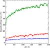 |
Fig. 10 Probability, Ptrans, that the source state is found changed a time interval Δt after a previous state determination for the different states (blue: hard; green: intermediate; red: soft) using ASM data. |
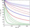 |
Fig. 11 The probability, 1 − Pct,n, that the source has remained in the same state (blue: hard; green: intermediate; red: soft) for at least the time Δt for different values of n of ignored number of possible outliers/misclassifications (n = 0: solid; n = 4: dashed; n = 8: dot-dashed; n = 12: dot-dot-dashed). The gray dashed line represents 0. |
Section 4.1 highlights that the different states are clearly different in their stability. While the source tends to remain in the hard and the soft states for a prolonged time, not unexpectedly the intermediate state is far more unstable. This well known general behavior can be quantified using the RXTE-ASM data, i.e., the data set in our measurements that covers the longest time span, does not have gaps, and can be reliably used to define all three states.
To calculate the state statistics, we calculate the probabilities that Cyg X-1 has changed its state after a certain interval and that the source remained in the same state throughout this interval for each ASM data point measured at a reference time, tref. More formally, we calculated the transited fraction, Ptrans, i.e., the probability that an observation made a certain time after the reference observation will find Cyg X-1 in a different source state (Fig. 10). The probability that the source state is unchanged is 1 − Ptrans. We determined Ptrans by calculating the fraction of all measurements in a different state than the reference measurement made at times ti with Δt1 ≤ ti − tref < Δt2 where {Δt1,Δt2} ∈ {{0 h, 1.5 h}, {1.5 h,3.0 h}, {3.0 h, 4.5 h},...}. This approach is equivalent to the one employed in Sect. 3.4, where we used RXTE spectra as reference measurements.
The transited fraction, Ptrans, does not take into account the possibility that the source might have undergone state changes between tref and ti. To address this possibility we calculated the cumulative transited fraction, Pct,n, which measures the probability that at least one source transition has happened up to a time interval Δt after the reference measurement. In order to assess the influence of possible outliers and/or misclassifications, we defined a state transition by the existence of more than n ∈ {0,..., 12} measurements in a different state than the reference measurement in the time interval tref ≤ t < tref + Δt. The probability that the source has remained in the same state for at least a time Δt is then given by 1 − Pct,n (Fig. 11).
As expected from a simple look at the light curves (see Fig. 1), hard states are the most stable states: in more than 90% of all cases, the source is still in the hard state 200 h after a given hard state ASM measurement (Fig. 10). In over 30% of all cases, a period of 300 h after any given hard state measurement will not contain even a single measurement in a different state. This number increases to over 70% for larger n, i.e., when very short excursions to the soft/intermediate state and/or outliers due to misclassifications are ignored (Fig. 11).
Though less stable and shorter than hard states, soft states generally show similar behavior. Even for n = 0, a significant number of soft state measurements are not followed by a state transition within 300 h, i.e., prolonged stable, soft states lasting more than 12 days exist. Such states are observed by ASM in periods i and iii (Fig. 1). MAXI and BAT data suggest an increased occurrence of such stable soft states also in period v.
The intermediate state behaves differently. The transited fraction strongly increases within the first few hours. Already fifty hours after a reference intermediate measurement about half of the measurement will show the source in a different state. The cumulative transited fraction approaches 100% even for n = 12 at 300 d (Fig. 11). Intermediate states are therefore short and unstable compared to hard and soft states.
5. Summary
Based on pointed RXTE observations, we have provided criteria to define X-ray states (hard, intermediate, and soft) using light curves from all sky monitor instruments. In particular we have shown that:
-
due to the complex source behavior, simple state definitions based just on the source count rate or just on the hardness do not adequately describe states;
-
a combination of RXTE-ASM total count rate and hardness can be used to define states before MJD 55200 (see Table 2 for exact cut);
-
the best separation of states is achieved with simultaneous ASM data. Data within Δt ±6 h result in a contamination of <10% for the hard and soft states and <30% for the intermediate state;
-
a combination of MAXI count rate and hardness can be used to define states (see Table 2 for exact cuts);
-
soft coverage is needed to define states and the lack of such does not allow the hard and the intermediate states to be distinguished using publicly available BAT light curves. BAT light curves can, however, be used to distinguish the soft state from hard/intermediate states: the source is in the soft state below a threshold of 0.09 counts cm-2 s-1, and in the hard/intermediate state above it (Table 2);
-
the lack of soft coverage does not allow a separation between hard and intermediate states with publicly available GBM data, with the analysis being further hindered by the low time resolution of the GBM ligh tcurve, but a rough state classification is to consider Cyg X-1 in the soft state for fluxes <0.6 Crab and in the hard/intermediate state above that threshold (Table 2);
-
the hard state is by far the most stable state of Cyg X-1, followed by the soft state. The probability that the source remains in the hard state for at least one week (200 h) is >85% (using Pct,12). Soft states are slightly less stable, but the probability of a soft state being longer than one week is still ~75%. Intermediate states are short-lived and typically last a few days at most, implying that they can only be caught with monitor data with a time resolution of better than 1 d.
The state classification introduced here can be reliably used to define source states where no X-ray continuum spectrum measurement is available. The high frequency of all sky monitor measurements for RXTE-ASM, Swift-BAT, and MAXI enables us to catch short flares and especially quick state transitions.
Vrtilek & Boroson (2013) come to similar conclusions regarding ASM data from 2010 on and report gain changes in the last two years of ASM lifetime as a possible cause.
Over its lifetime the PCA saw four different gain and calibration epochs, followed by a long fifth epoch defined by the loss of the propane layer in PCU0 in 2000 May. See http://heasarc.gsfc.nasa.gov/docs/xte/e-c_table.html for details. These epochs are not to be confused with the five activity periods of Cyg X-1 that we define in Fig. 1 and Sect. 3.1.
Since the PCA data in the lower channels are dominated by systematic errors for a source as bright as Cyg X-1, it is not possible to adopt a significance-based criterion for the improvement in χ2.
Zdziarski et al. (2011b) define the soft state according to a power-law photon index deduced from the ASM count rates. This approach does not exactly correspond to the approach chosen here, however, it is similar enough to allow rough comparisons.
Acknowledgments
This work has been partially funded by the Bundesministerium für Wirtschaft und Technologie under Deutsches Zentrum für Luft- und Raumfahrt Grants 50 OR 1007 and 50 OR 1113 and by the European Commission through ITN 215212 “Black Hole Universe”. It was partially completed by LLNL under Contract DE-AC52-07NA27344, and is supported by NASA grants to LLNL and NASA/GSFC. This research has made use of the MAXI data provided by RIKEN, JAXA and the MAXI team. We thank John E. Davis for the development of the slxfig module used to prepare all figures in this work. V.G. thanks NASA’s Goddard Space Flight Center for its hospitality during the time when the research presented here was done. V.G. and M.C.B. acknowledge support from the Faculty of the European Space Astronomy Centre (ESAC).
References
- Bałucińska-Church, M., Church, M. J., Charles, P. A., et al. 2000, MNRAS, 311, 861 [NASA ADS] [CrossRef] [Google Scholar]
- Barthelmy, S. D., Barbier, L. M., Cummings, J. R., et al. 2005, Space Sci. Rev. 120, 143 [NASA ADS] [CrossRef] [Google Scholar]
- Belloni, T. M. 2010, In Lect. Notes Phys. (Berlin: Springer Verlag), 794, 53 [NASA ADS] [CrossRef] [Google Scholar]
- Benlloch, S., Pottschmidt, K., Wilms, J., et al. 2004, In X-ray Timing 2003: Rossi and Beyond, eds. P. Kaaret, F. K. Lamb, & J. H. Swank, AIP Conf. Ser., 714, 61 [Google Scholar]
- Böck, M., Grinberg, V., Pottschmidt, K., et al. 2011, A&A, 533, A8 [NASA ADS] [CrossRef] [EDP Sciences] [Google Scholar]
- Boroson, B., & Vrtilek, S. D. 2010, ApJ 710, 197 [NASA ADS] [CrossRef] [Google Scholar]
- Brocksopp, C., Fender, R. P., Larionov, V., et al. 1999a, MNRAS, 309, 1063 [NASA ADS] [CrossRef] [Google Scholar]
- Brocksopp, C., Tarasov, A. E., Lyuty, V. M., & Roche, P. 1999b, A&A, 343, 861 [NASA ADS] [Google Scholar]
- Case, G. L., Cherry, M. L., Wilson-Hodge, C. A., et al. 2011, ApJ, 729, 105 [NASA ADS] [CrossRef] [Google Scholar]
- Fender, R. P., Belloni, T. M., & Gallo, E. 2004, MNRAS, 355, 1105 [NASA ADS] [CrossRef] [Google Scholar]
- Fender, R. P., Stirling, A. M., Spencer, R. E., et al. 2006, MNRAS, 369, 603 [NASA ADS] [CrossRef] [Google Scholar]
- Fender, R. P., Homan, J., & Belloni, T. M. 2009, MNRAS, 396, 1370 [NASA ADS] [CrossRef] [Google Scholar]
- Fürst, F., Wilms, J., Rothschild, R. E., et al. 2009, Earth Planet. Sci. Lett. 281, 125 [NASA ADS] [CrossRef] [Google Scholar]
- Gies, D. R., Bolton, C. T., Blake, R. M., et al. 2008, ApJ, 678, 1237 [NASA ADS] [CrossRef] [Google Scholar]
- Hanke, M. 2011, Ph.D. Thesis, Universität Erlangen-Nürnberg [Google Scholar]
- Hanke, M., Wilms, J., Nowak, M. A., et al. 2009, ApJ, 690, 330 [NASA ADS] [CrossRef] [Google Scholar]
- Houck, J. C. 2002, In High Resolution X-ray Spectroscopy with XMM-Newton and Chandra, ed. G. Branduardi-Raymont, published electronically [Google Scholar]
- Houck, J. C., & Denicola L. A. 2000, In Astronomical Data Analysis Software and Systems IX, eds. N. Manset, C. Veillet, & D. Crabtree, ASP Conf. Ser., 216, 591 [Google Scholar]
- Ibragimov, A., Zdziarski, A. A., & Poutanen, J. 2007, MNRAS, 381, 723 [NASA ADS] [CrossRef] [Google Scholar]
- Jahoda, K., Markwardt, C. B., Radeva, Y., et al. 2006, ApJS, 163, 401 [NASA ADS] [CrossRef] [Google Scholar]
- Jourdain, E., Roques, J. P., Chauvin, M., & Clark, D. J. 2012, ApJ, 761, 27 [NASA ADS] [CrossRef] [Google Scholar]
- Körding, E., Rupen, M., Knigge, C., et al. 2008, Science, 320, 1318 [NASA ADS] [CrossRef] [PubMed] [Google Scholar]
- Körding, E. G., Jester, S., & Fender, R. 2006, MNRAS, 372, 1366 [NASA ADS] [CrossRef] [Google Scholar]
- Laurent, P., Rodriguez, J., Wilms, J. et al. 2011, Science, 332, 438 [NASA ADS] [CrossRef] [PubMed] [Google Scholar]
- Levine, A. M., Bradt, H., Cui, W., et al. 1996, ApJ, 469, L33 [NASA ADS] [CrossRef] [Google Scholar]
- Maitra, D., & Bailyn, C. D. 2004, ApJ, 608, 444 [NASA ADS] [CrossRef] [Google Scholar]
- Makishima, K., Maejima, Y., Mitsuda, K., et al. 1986, ApJ, 308, 635 [NASA ADS] [CrossRef] [Google Scholar]
- Matsuoka, M., Kawasaki, K., Ueno, S., et al. 2009, PASJ, 61, 999 [NASA ADS] [CrossRef] [Google Scholar]
- McClintock, J. E., & Remillard, R. A. 2006, In Compact Stellar X-ray Sources (Cambridge University Press), 157 [Google Scholar]
- Meegan, C., Bhat, N., Connaughton, V., et al. 2007, In The First GLAST Symposium, eds. S. Ritz, P. Michelson, & C. A. Meegan, AIP Conf. Ser., 921, 13 [Google Scholar]
- Mitsuda, K., Inoue, H., Koyama, K., et al. 1984, PASJ, 36, 741 [NASA ADS] [Google Scholar]
- Noble, M. S., & Nowak, M. A. 2008, PASP, 120, 821 [NASA ADS] [CrossRef] [Google Scholar]
- Nowak, M. A., Vaughan, B. A., Wilms, J., et al. 1999, ApJ, 510, 874 [NASA ADS] [CrossRef] [Google Scholar]
- Nowak, M. A., Hanke, M., Trowbridge, S. N., et al. 2011, ApJ, 728, 13 [NASA ADS] [CrossRef] [Google Scholar]
- Pooley, G. G., Fender, R. P., & Brocksopp, C. 1999, MNRAS, 302, L1 [NASA ADS] [CrossRef] [Google Scholar]
- Pottschmidt, K., Wilms, J., Nowak, M. A., et al. 2000, A&A, 357, L17 [NASA ADS] [Google Scholar]
- Pottschmidt, K., Wilms, J., Nowak, M. A., et al. 2003, A&A, 407, 1039 [NASA ADS] [CrossRef] [EDP Sciences] [Google Scholar]
- Poutanen, J., Zdziarski, A. A., & Ibragimov, A. 2008, MNRAS, 389, 1427 [NASA ADS] [CrossRef] [Google Scholar]
- Reid, M. J., McClintock, J. E., Narayan, R., et al. 2011, ApJ, 742, 83 [NASA ADS] [CrossRef] [Google Scholar]
- Remillard, R. A. 2005, In SLAC Electronic Conference Proceedings Archive, ed. P. Chen, Texas@Stanford 2004 [astro-ph/0504129] [Google Scholar]
- Rothschild, R. E., Blanco, P. R., Gruber, D. E., et al. 1998, ApJ, 496, 538 [NASA ADS] [CrossRef] [Google Scholar]
- Stirling, A. M., Spencer, R. E., de la Force, C. J., et al. 2001, MNRAS, 327, 1273 [NASA ADS] [CrossRef] [Google Scholar]
- von Kienlin, A., Meegan, C. A., Lichti, G. G., et al. 2004, In UV and Gamma-Ray Space Telescope Systems, eds. G. Hasinger, & M. J. L. Turner, SPIE Conf. Ser., 5488, 763 [Google Scholar]
- Vrtilek, S. D., & Boroson, B. S. 2013, MNRAS, 428, 3693 [NASA ADS] [CrossRef] [Google Scholar]
- Wilms, J., Allen, A., & McCray, R. 2000, ApJ, 542, 914 [NASA ADS] [CrossRef] [Google Scholar]
- Wilms, J., Nowak, M. A., Pottschmidt, K., et al. 2006, A&A, 447, 245 [NASA ADS] [CrossRef] [EDP Sciences] [Google Scholar]
- Wilms, J., Pottschmidt, K., Pooley, G. G., et al. 2007, ApJ, 663, L97 [NASA ADS] [CrossRef] [Google Scholar]
- Wilson-Hodge, C. A., Cherry, M. L., Case, G. L., et al. 2011, ApJ, 727, L40 [NASA ADS] [CrossRef] [Google Scholar]
- Wilson-Hodge, C. A., Case, G. L., Cherry, M. L., et al. 2012, ApJS, 201, 33 [NASA ADS] [CrossRef] [Google Scholar]
- Xiang, J., Lee, J. C., Nowak, M. A., & Wilms, J. 2011, ApJ, 738, 78 [NASA ADS] [CrossRef] [Google Scholar]
- Zdziarski, A. A., Poutanen, J., Paciesas, W. S., & Wen, L. 2002, ApJ, 578, 357 [NASA ADS] [CrossRef] [Google Scholar]
- Zdziarski, A. A., Pooley, G. G., & Skinner, G. K. 2011a, MNRAS, 412, 1985 [NASA ADS] [CrossRef] [Google Scholar]
- Zdziarski, A. A., Skinner, G. K., Pooley, G. G., & Lubiński, P. 2011b, MNRAS, 416, 1324 [NASA ADS] [CrossRef] [Google Scholar]
All Tables
Spearman’s rank correlation coefficients ρ between the ASM counts and the soft photon index Γ1
Time Cyg X-1 spent in the different states (hard − H, intermediate − I, soft − S) as measured by the RXTE-ASM, Swift-BAT, MAXI, and Fermi-GBM all sky monitors.
All Figures
|
Fig. 1 Pointed RXTE observations and all light curves (RXTE-ASM, MAXI, Swift-BAT, and GBM) of Cyg X-1 used in this analysis. ASM, MAXI, and BAT data are shown in the highest available resolution, GBM are binned daily. ASM hardness is calculated by dividing count rates in band C (5.0−12 keV) by count rates in band A (1.5−3.0 keV). Vertical dashed lines and horizontal arrows represent periods of different source activity patterns. Blue, green, and red colors represent states of individual measurements classified using the respective classification for the different instruments as introduced in Sect. 3: blue represents the hard state, green the intermediate state and red the soft state. ASM data after MJD 55200 (shown in gray) are affected by intrumental decline. Hard and intermediate states cannot be separated in BAT and GBM; BAT and GBM data corresponding to these periods of hard or intermediate states are therefore shown in black. |
| In the text | |
|
Fig. 2 Crab ASM light curve (left panel, 1.5−12 keV, gray points) and hardness (right panel, 5.0−12 keV/1.5−3.0 keV, gray points) with the respective 10-day average values (black histograms) and variances (blue histograms). |
| In the text | |
|
Fig. 3 X-ray time lag and fractional rms as a function of the soft photon index Γ1. |
| In the text | |
|
Fig. 4 Dependence of the ASM count rate in different bands on the soft photon index Γ1 of simultaneous pointed RXTE observations. Shown are total ASM counts (1.5−12 keV, black dots) and counts in the three ASM energy bands: band A (1.5−3 keV, orange upside down triangles), band B (3−5 keV, green triangles), and band C (5−12 keV, magenta squares). |
| In the text | |
|
Fig. 5 PCA to ASM mapping. Gray data points are all ASM measurements of Cyg X-1 in the shown range. Blue points represent PCA defined hard states, green intermediate and red soft states. Black lines show the cuts defining the states in the ASM HID. The light blue shaded region corresponds to the position of the hard state in the HID, the light red shaded to the position of the soft state. The intermediate state region is shown without shading. |
| In the text | |
|
Fig. 6 Percentage of contamination of the ASM defined states (hard state shown in blue, intermediate in green, and soft in red) for time delays Δt = ± (0–1.5) h, ± (1.5–3) h, ± (3–4.5) h, etc., between the ASM and the pointed RXTE measurements. Simple linear fits to the data are shown as dashed lines to illustrate the overall trends. |
| In the text | |
|
Fig. 7 PCA to MAXI mapping. Gray data points are all MAXI orbitwise measurements of Cyg X-1 in the shown energy range. Blue circles represent Γ1-defined hard states, green intermediate states and red soft states. Black lines define the state cuts. The light blue shaded region corresponds to the hard state in the MAXI HID, the light red shaded region to the soft state, and the region without shading to the intermediate state. |
| In the text | |
|
Fig. 8 Histogram of BAT fluxes of Γ1-defined states. The hard state is shown in blue, the intermediate state in green, and the soft state in red. |
| In the text | |
|
Fig. 9 Left: daily GBM HID. S denotes the 12−25 keV flux, H the 25−50 keV flux. The gray dashed line denotes the zero flux level. Total GBM measurements are shown in gray. Right: histogram of daily GBM fluxes of Γ1-defined states. The hard state is shown in blue, intermediate state in green, and soft state in red. Total GBM measurement are shown in black. The gray dashed line denotes the zero flux level. |
| In the text | |
|
Fig. 10 Probability, Ptrans, that the source state is found changed a time interval Δt after a previous state determination for the different states (blue: hard; green: intermediate; red: soft) using ASM data. |
| In the text | |
|
Fig. 11 The probability, 1 − Pct,n, that the source has remained in the same state (blue: hard; green: intermediate; red: soft) for at least the time Δt for different values of n of ignored number of possible outliers/misclassifications (n = 0: solid; n = 4: dashed; n = 8: dot-dashed; n = 12: dot-dot-dashed). The gray dashed line represents 0. |
| In the text | |
Current usage metrics show cumulative count of Article Views (full-text article views including HTML views, PDF and ePub downloads, according to the available data) and Abstracts Views on Vision4Press platform.
Data correspond to usage on the plateform after 2015. The current usage metrics is available 48-96 hours after online publication and is updated daily on week days.
Initial download of the metrics may take a while.