| Issue |
A&A
Volume 554, June 2013
|
|
|---|---|---|
| Article Number | A77 | |
| Number of page(s) | 11 | |
| Section | The Sun | |
| DOI | https://doi.org/10.1051/0004-6361/201220947 | |
| Published online | 11 June 2013 | |
Magnetohydrodynamic simulations of the ejection of a magnetic flux rope⋆
1 School of Mathematics and Statistics, University of St Andrews, North Haugh, St Andrews, Fife, Scotland KY16 9SS, UK
e-mail: This email address is being protected from spambots. You need JavaScript enabled to view it.
2 Centre for Plasma-Astrophysics, K. U. Leuven, Celestijnenlaan 200B, 3001 Leuven, Belgium
Received: 18 December 2012
Accepted: 20 March 2013
Abstract
Context. Coronal mass ejections (CME’s) are one of the most violent phenomena found on the Sun. One model to explain their occurrence is the flux rope ejection model. In this model, magnetic flux ropes form slowly over time periods of days to weeks. They then lose equilibrium and are ejected from the solar corona over a few hours. The contrasting time scales of formation and ejection pose a serious problem for numerical simulations.
Aims. We simulate the whole life span of a flux rope from slow formation to rapid ejection and investigate whether magnetic flux ropes formed from a continuous magnetic field distribution, during a quasi-static evolution, can erupt to produce a CME.
Methods. To model the full life span of magnetic flux ropes we couple two models. The global non-linear force-free field (GNLFFF) evolution model is used to follow the quasi-static formation of a flux rope. The MHD code ARMVAC is used to simulate the production of a CME through the loss of equilibrium and ejection of this flux rope.
Results. We show that the two distinct models may be successfully coupled and that the flux rope is ejected out of our simulation box, where the outer boundary is placed at 2.5 R⊙. The plasma expelled during the flux rope ejection travels outward at a speed of 100 km s-1, which is consistent with the observed speed of CMEs in the low corona.
Conclusions. Our work shows that flux ropes formed in the GNLFFF can lead to the ejection of a mass loaded magnetic flux rope in full MHD simulations. Coupling the two distinct models opens up a new avenue of research to investigate phenomena where different phases of their evolution occur on drastically different time scales.
Key words: Sun: coronal mass ejections / Sun: corona / magnetic fields / magnetohydrodynamics (MHD)
Movies are available in electronic form at http://www.aanda.org
© ESO, 2013
1. Introduction
Coronal mass ejections (CMEs) are one of the few solar phenomena that directly affect the Earth, therefore they are one of the main drivers of space weather (Schwenn 2006). Understanding their origin and propagation is therefore key, not only for the Earth but also for understanding how the Sun loses both magnetic flux and magnetic helicity (Low 1996; Lynch et al. 2005). Over the years, a wide variety of models have been put forward to explain the origin of CMEs, and a discussion of these can be seen in the reviews of Forbes et al. (2006) and Chen (2011). While a variety of models exist, one of the leading models for explaining CMEs is the flux rope ejection model (Forbes & Isenberg 1991; Amari et al. 2000; Fan & Gibson 2007). The flux rope ejection model may itself be split into two categories. Flux ropes formed quasi-statically from perturbations of already existing coronal arcades (Aulanier et al. 2005; Mackay & van Ballegooijen 2006a) or those formed dynamically during the emergence of magnetic flux (Manchester et al. 2004; Archontis & Hood 2008). Within the present paper we focus on those formed quasi-statically from existing coronal arcades.
For this category of flux rope, the life span normally undergoes three separate stages of evolution: the formation, equilibrium and eruption phases. To begin with, the flux rope forms over time periods of days to weeks as a coronal arcade is perturbed by photospheric motions and flux cancellation at a PIL (van Ballegooijen & Martens 1989; Forbes 1991). An example can be seen in Cheng et al. (2010) where the flux rope formation was observed over three days, along with the signature of flux cancellation at the photosphere. Similar dynamics have been observed by Liu et al. (2010), where a sigmoidal flux rope was formed by the joining of two J-shaped loops which then quickly erupt. The formation phase is then followed by a period during which the flux rope lies in near equilibrium with its surroundings. Evidence for this exists in the form of sigmoids (McKenzie & Canfield 2008), solar filaments (Mackay et al. 2010), and coronal cavities (Hudson et al. 1999). During both the formation and equilibrium phases the magnetic structure does not change significantly over time scales much longer than the characteristic Alfvén time.
Finally, there is the ejection phase where the flux rope loses equilibrium and is ejected out of the solar corona due to magnetic forces. This occurs over time periods of a few hours, where flux rope ejections are believed to be one of the main progenitors of CMEs. It is possible to track the evolution of a flux rope in observed CMEs from the ejection phase (Cheng et al. 2011) to their propagation into interplanetary space (Wood et al. 1999). While many flux ropes follow the evolution described above, there are also situations where flux ropes are simultaneously formed and ejected (Cheng et al. 2011; Archontis et al. 2009).
It can be seen that the formation and ejection of magnetic flux ropes involve a wide variety of time scales. The formation phase happens very slowly (days to weeks or months). Under these circumstances the formation can be approximated using a quasi-static zero-β model where the magnetic field evolves through a series of equilibrium states (Forbes 1991; Mackay & van Ballegooijen 2006a,b; Yeates & Mackay 2009; Yeates et al. 2010). In contrast the ejection phase is rapid, where a flux rope can travel at the speed of several hundreds of km s-1 and within a few hours the coronal magnetic field reconfigures to a state significantly different from the pre-eruption state. One important aspect of the ejection is that the coronal plasma is compressed and heated. As a result, the plasma may no longer be in the low β-regime and full MHD modelling must now be applied.
The wide variety of time scales involved, in the formation of the flux rope and then its eruption, poses a considerable challenge to theoretical models. Within the present paper our aim is to combine two models, which we believe accurately reproduce individual aspects of flux rope formation and ejection over their individual time scales. We will first use the global non-linear force-free field (GNLFFF) model of Mackay & van Ballegooijen (2006a) which neglects the role of the plasma to consider the formation of the flux rope in the zero-β, quasi-static approximation. Once the flux rope forms and is about to erupt, we apply a full MHD approach, through using the stressed magnetic field configuration from the GNLFFF model as an initial condition in MHD simulations using the AMRVAC code (Keppens et al. 2012). With this we can accurately describe the full life span of the evolution of a flux rope from its slow generation to its rapid ejection.
While we choose to apply these two methods, full MHD simulations may in principle be used to simulate both the formation and eruption of the flux rope. However, presently this is not practicable for two reasons. The first is limited computational resources. To model only the eruptive phase which corresponds to approximately two hours of physical time, we require over 5000 cpu hours. If we were to model the full three weeks of formation and ejection, assuming a linear scaling, we would need three months for a single run. Additionally due to the small MHD signal travel time, a large number of iterations would be required over the three months of computation. This would significantly increase round-off errors and numerical diffusion in the AMRVAC code.
While our approach is one way of considering the origin of CMEs, other authors have tackled the modelling of flux rope ejections using different approaches. An example is that of Reeves et al. (2010) who modelled a solar eruption as the outcome of a slow evolution preceding a fast and sudden eruption. In addition, a number of authors have considered alternative methods for forming flux ropes which do not use flux cancellation. For example, Fan (2009) and Archontis et al. (2009) explain the flux rope formation in the framework of flux emergence. Savcheva et al. (2012) explain the formation of an observed flux rope due to the rotation of the foot points of an active region in the presence of magnetic diffusion. While in Amari et al. (2003) the flux rope is formed (and then ejected) as a result of shearing followed by flux cancellation. In addition to these studies, the ejection of flux ropes may be explained by several mechanisms in numerical models: Török & Kliem (2005, 2007), Fan (2010) and Aulanier et al. (2010) use the Torus instability as the main driver for a full ejection. Archontis & Hood (2012) describes the eruption of a flux rope in the context of flux emergence with an horizontal ambient magnetic field antiparallel to the emerging magnetic field (see also Antiochos et al. 1999). Roussev et al. (2012) consider the solar eruption as a reorganization of the solar corona after magnetic flux and helicity injection. Finally, in Amari et al. (2011) the convergence of foot points causes the ejection.
While there are the many models for the formation and ejection of flux ropes we have decided to focus only on the flux cancellation model in this paper, as first described by van Ballegooijen & Martens (1989) and simulated by Mackay & van Ballegooijen (2006a). An important aspect of this work is that we form the flux rope out of a smoothly varying continuous magnetic field configuration, which is different from many other techniques. This means that the coronal magnetic field is not predisposed to allow reconnection, as happens in some models which use distinct flux configurations. The outline of the paper is as follows. The coupling of the GNLFFF and the MHD models is non-trivial and will be explained in detail in Sect. 2 with additional information in Appendices A and B. In Sect. 3 we describe the outcome of our MHD simulation which produces the ejection of the flux rope. In Sect. 4 we discuss the results and finally draw conclusions in Sect. 5. It should be noted that this is the first stage in this process where we have made a number of simplifications due to the new technique being employed. In future studies these assumptions will be relaxed.
2. Method
2.1. Previous simulations
In order to pursue the objective of modelling the full life span of a flux rope from the slow quasi-static built-up to the rapid ejection, we adopt two different numerical models for the two different phases in the life of a flux rope. We couple the two techniques through using the output from one model as the initial condition for the other.
Mackay & van Ballegooijen (2006a) apply a GNLFFF model that produces flux ropes by means of the relative motion and interaction of two magnetic bipoles. In the model, one bipole is slightly more tilted with respect to the equator than the other. The two bipoles are then advected under the effect of solar differential rotation, meridional flow and surface diffusion. Differential rotation has the effect of shearing the magnetic field lines of the bipoles and produces an axial magnetic field over the PIL. This axial magnetic field is then localized above the PIL due to surface diffusion. As a result of flux cancellation a flux rope forms above the PIL of the more tilted bipole after 19 days of evolution. An illustration of this 3D magnetic field configuration at the time of flux rope formation can be seen in Fig. 1. An important aspect of this 3D magnetic field with flux rope is that it is produced out of a continuous magnetic field and in the area surrounding the flux rope no antiparallel magnetic field lines exist.
We identify this as the time when a flux rope has clearly formed in the simulation. If the GNLFFF simulation is continued, the newly formed flux rope becomes unstable and is ejected out of the computational box (a full description is given in Mackay & van Ballegooijen 2006a,b). However, the simulations of Mackay & van Ballegooijen (2006a) neglect the effect of the plasma and use a magnetic relaxation technique, so the ejection of the flux rope does not follow the true dynamics of an erupting system. In particular the time scale of the ejection is too slow compared to an observed eruption. For the purposes of the present paper we assume the evolution modelled by Mackay & van Ballegooijen (2006a) to be accurate until day 19. We then adopt the stressed non-potential magnetic field that exists on this day as the initial magnetic field condition for numerical MHD simulations using ARMVAC which will follow the dynamics of the eruption.
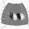 |
Fig. 1 Configuration of the magnetic field after 19 days of evolution using the model of Mackay & van Ballegooijen (2006a). The figure shows a sample of magnetic field lines that illustrate the structure of the magnetic bipoles, the overlying arcade, and the newly formed magnetic flux rope along the PIL of the left-hand side bipole. The surface boundary is coloured according to the polarity of the magnetic field: negative polarity is black and positive is white. |
The coupling of the two models is a non-trivial process and is a major technical challenge of the presented work. In order to accomplish this some assumptions and approximations are required (Sect. 2.2). From a mere technical point of view, the successful combination of these two modelling techniques is an achievement which produces a new tool for long term studies.
2.2. Coupling of the two models
To couple the two models we need to generate a full set of MHD variables (density ρ, velocity v, total energy density e and magnetic field B = ∇ × A) from the GNLFFF variables (vector potential A and magnetic field B). In both codes the variables are defined in the spherical domain (r, θ, φ). However, only the magnetic field, B, is common to both codes (see Fig. 2). The three components of the magnetic field are therefore directly transported from the GNLFFF code to the MHD code as described in Appendix A. The transport is designed to preserve the gradients of B, thus the forces in the system. However for the other MHD variables assumptions need to be made.
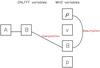 |
Fig. 2 Illustration of the coupling of the GNLFFF variables as input for the MHD code. We interpolate the magnetic field B of the GNLFFF model for use in the MHD code. From B we then deduce the density. The velocity is then automatically created in the MHD code and thermal pressure set. |
As the velocity, v, in the GNLFFF model, is a non-physical relaxation velocity we do not import it into the MHD simulation. We choose to initially set v = 0 in the MHD model. However for cases where the imported magnetic field is not in equilibrium a non-zero velocity develops within the MHD simulation after one time step. To complete the set of MHD variables, we assume that the density of the plasma, ρ, is given by 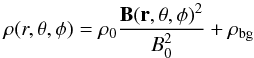 (1)where we include a background uniform distribution to avoid extremely low density values occurring where the magnetic field is weak. Typical parameters are chosen to be ρ0 = 10-17 g/cm3, B0 = 1 G, ρbg = 10-21 g/cm3. We also assume a uniform thermal pressure, p,
  (2)where p0 = 0.006 dyne/cm2.
2.3. ARMVAC code
Once we have a full set of MHD variables from the coupling of the models, we perform a MHD simulation. An important feature of our MHD simulations is that no photospheric boundary motions are applied. This means that any dynamics occurring within the MHD simulation are purely due to the stress developed in the GNLFFF simulation before the data is transferred into the MHD simulation. We use the AMRVAC code mainly developed at the KU Leuven to run the simulations (Keppens et al. 2012). The code solves the MHD equations in their conservative form and we make use of the magnetic field splitting technique (Powell et al. 1999) and consider 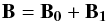 (3)where B0 is a static, intrinsic magnetic field and B1 is the difference (B − B0). The following equations must hold for B0
 The MHD equations we solve are
 ![Mathematical equation: \begin{eqnarray} \label{mass} &&\frac{\partial\rho}{\partial t}=-\vec{\nabla}\cdot(\rho\vec{v}) \\ \label{momentum} &&\frac{\partial\rho\vec{v}}{\partial t}+\vec{\nabla}\cdot(\rho\vec{v}\vec{v})= -\nabla p+\frac{(\vec{\nabla}\times\vec{B_1})\times(\vec{B_0}+\vec{B_1})}{4\pi} \\ \label{induction} &&\frac{\partial\vec{B_1}}{\partial t}=\vec{\nabla}\times(\vec{v}\times(\vec{B_0}+\vec{B_1})) \\ \label{energy} &&\frac{\partial e}{\partial t}+\vec{\nabla}\cdot[(e+p)\vec{v}]=0 \end{eqnarray}](/articles/aa/full_html/2013/06/aa20947-12/aa20947-12-eq31.png)
where the expression for the total energy density e is  (11)and γ = 5/3 is the ratio of specific heats, and t is the time.
The use of the magnetic field splitting technique allows us to remove any errors that arise when transporting the variables from the GNLFFF code to the MHD code, due to round-off, discretization, and truncation. In effect, it minimizes spurious forces that are numerically generated. In addition, by neglegting the energy associated to the  term in Eq. (11) we avoid the thermal pressure being a residual subject to round off errors where the plasma β is extremely low.
In our simulation, B0 is chosen to be the potential field deduced from the photospheric magnetic field from the GNLFFF simulation, and B1 is simply computed as the difference between B of the GNLFFF and the prescribed B0. Given the specified photospheric magnetic field, the resulting coronal potential magnetic field is unique.
To check the stability of this technique, we have performed several simulations with different B0 and therefore B1 (corresponding to the same B). Different choices of B0 corresponds to different choices of the photospheric magnetic field compared to that transported from the GNLFFF model. The smaller B1 becomes, the less magnetic flux is free to numerically reconnect. The potential magnetic field B0 derived from the photospheric magnetic field at Day 19 of the GNLFFF simulation is the most natural choice, in order to have the smallest B1, however the potential magnetic field derived from any photospheric magnetic field of the GNLFFF is a suitable B0.
In the simulation we present here, the numerical diffusion has no role in driving the early evolution of the system, which is solely due to the initial condition being out of magnetohydrostatic equilibrium, i.e. the initial evolution is the same and independent of the choice of B0. On the other hand, after tenths of Alvén times (~30), if the system has highly departed from the initial condition, the exact evolution of the system does depend to some degree on how the magnetic field numerically reconnects and the initial choice of B0 can play a role. It should however be noted that in all simulations the ejection progresses in a similar manner no matter the choice of B0. The simulation we present here is for the smallest B1 possible.
To evolve the system of Eqs. (7)−(10) forward in time we use a Total Variation Diminishing Lax-Friedrichs scheme (Tóth & Odstrcil 1996).
The size of the computational domain is the same as in the GNLFFF model where it extends over 1.5 R⊙ in radial extent starting from r = R⊙. The colatitude, θ, spans from θ = 30° to θ = 100° and the longitude, φ, spans over 90°. The boundary conditions are treated with a system of ghost cells. Open boundary conditions are imposed at the outer boundary, reflective boundary conditions are set at the θ boundaries and the φ boundaries are periodic. At the lower boundary we impose constant boundary conditions taken from the first four θ-φ planes of cells derived from the GNLFFF model. Therefore the actual computational domain is composed of 128 × 128 × 128 cells. The validity of the technique to combine the two models is tested in Appendix B through importing an equilibrium magnetic field configuration.
3. Simulations of an erupting flux rope
3.1. Properties of the initial condition
 |
Fig. 3 Magnetic field configuration used as the initial condition in the MHD simulations of the erupting flux rope. Red lines represent the flux rope, blue lines the arcades, green lines the external magnetic field. The lower boundary is coloured according to the intensity of the magnetic field from red (strong) to blue (weak) in arbitrary units. |
Figure 3 illustrates the initial condition for the magnetic field in the MHD simulation of the erupting flux rope which comes from day 19 of the simulations of Mackay & van Ballegooijen (2006a). The magnetic field lines of the flux rope connect between the two polarities of the left hand side (LHS) bipole (red lines, Fig. 3). Overlying the flux rope, magnetic field lines create an arcade like structure. Three additional arcade systems are also present in the initial condition: one above the Right Hand Side (RHS) bipole, another connecting between the two bipoles (both shown as blue lines in Fig. 3) and finally an arcade lies high in the corona connecting between the external polarities of the bipoles (green lines, Fig. 3). The magnetic field configuration shown in Fig. 3 is a single smoothly varying continuous system.
In the lower corona where the magnetic field strength is approximately 10 Gauss, the prescribed initial density is around 10-16 g/cm3. The density drops by several orders of magnitude in the outer corona to a final value of 10-21 g/cm3 at 2.5 R⊙, where the magnetic field intensity is ~0.01 Gauss. The pressure is initially uniform (p = 0.006 dyne/cm2) and in the domain β ranges from 10-3 near the centre of the bipoles to 103 at the outer boundary. The initial Alfvén speed is of the order of 108 cm/s. The time step of the AMRVAC simulation is around dt = 5 × 10⁻³ s, and snapshots of the simulation are sampled every Δt ≈ 70 s, which corresponds to about half an Alfvén time (τAlf = 120 s). Hereafter we express the time in units of τAlf.
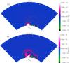 |
Fig. 4 Radial component of the Lorentz Force on the r − φ plane at the centre of the bipole at a) t = 0 τAlf and b) t = 23.20 τAlf. In panel b) the dashed black lines mark the contours of negative radial component of the Lorentz force at FLR = −2 × 10-11 dyne. Red lines represent some magnetic field lines. |
To understand how the pre-stressed initial condition of the magnetic field will drive the dynamics, Fig. 4a shows a map of the radial component of the Lorentz force in the r − φ plane along the centre of the bipoles. In all plots white/pink denote positive values, blue zero values and green/black negative values. It is clear from Fig. 4a that there is a strong positive (radially outward) component of the Lorentz force localized under and around the flux rope in the initial condition.
3.2. Early phase of the ejection
At t = 0 τAlf the positive Lorentz force present underneath the flux rope pushes the flux rope and the plasma contained within it upwards and it immediately starts to rise. Therefore the initial condition as imported from the GNLFFF model results in an erupting system. Simultaneously the foot points of the flux rope are subjected to a twisting motion due to the θ and φ components of the Lorentz force (not shown). As the flux rope moves up a horizontal Lorentz force acts below the flux rope to push oppositely oriented magnetic field lines on either side of the PIL towards the PIL. When these magnetic field lines encounter one-another they reconnect below the flux rope. This creates deeply dipped magnetic field lines which increase the outward component of the Lorentz force.
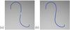 |
Fig. 5 Magnetic field lines departing from the same points of the LHS bipole polarity regions at a) t = 2.61 τAlf and b) t = 2.67 τAlf. |
Figure 5 illustrates this process, where in Fig. 5a we see two individual magnetic field lines at t = 2.61 τAlf. These magnetic field lines are typical of the arcade magnetic field lines that connect the outer and central part of the LHS bipole. These magnetic field lines are pushed towards one another and reconnect below the flux rope to produce a low, deeply dipped, magnetic field line underneath the flux rope. In Fig. 5b at t = 2.67 τAlf we see the reconnected magnetic field line where the magnetic field line has the same outer edge starting points as before. Through this process, by t = 2.67 τAlf the radial component of the Lorentz force under the flux rope doubles in magnitude compared to its initial value.
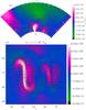 |
Fig. 6 a) Radial component of the velocity on the r − φ plane through the centre of the bipole at t = 11.6 τAlf. b) Radial component of the velocity on the θ − φ plane at r = 1.07 R⊙ at the same time with superimposed contours of the radial component of the magnetic field (black lines, dashed lines for negative values and solid lines for positive values) and the projection of the horizontal velocity field onto the same θ − φ plane (green arrows, typical velocity is 2 × 106 cm/s and minimum velocity shown is 1.3 × 106 cm/s). |
In Fig. 6 the bulk plasma velocity at t = 11.6 τAlf can be seen. Figure 6a shows a map of the radial component of the velocity in the r − φ plane, along the centre of the bipoles, while Fig. 6b shows a map of the radial component of the velocity in the θ − φ plane zoomed in at the bipoles. In addition, in Fig. 6b contours of the radial component of the magnetic field are shown (solid contours positive flux, dashed negative flux) and the green vectors denote the horizontal velocity field. In Fig. 6b the velocity vectors are typically of the order of 2 × 106 cm/s while velocity vectors of magnitude lower than 1.3 × 106 cm/s are not shown. Figure 6a shows that the plasma above the LHS bipole is ejected outwards with a velocity higher than 8 × 106 cm/s. This motion is initially due to the positive radial Lorentz force present under the flux rope in the initial condition and secondly due to the reconnection of the magnetic field lines below the flux rope. Figure 6b clearly shows that in the proximity of the PIL of the LHS bipole (above which the flux rope lies) the plasma moves upwards. Simultaneously horizontal plasma motions converge towards the PIL. The convergence is most prominent in the zone around θ = [70°,75°] and φ = [38°,42°].
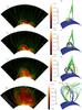 |
Fig. 7 a)−d) Maps of log 10(ρ) on the (φ,r) plane passing through the centre of the bipoles at different times. Super-imposed are magnetic field lines plotted from the same points (green lines) and a contour line at β = 1 (white line). e)−h) Magnetic configurations at the same times as the LHS column. Yellow magnetic field lines depart from the negative polarity of the LHS bipole, blue magnetic lines depart from the positive polarity of the LHS bipole, green magnetic lines represent the external magnetic field. All the magnetic field lines in panels a)−d) and e)−h) are plotted from the same starting points at all the times. |
To follow the ejection of the flux rope and the motion of the plasma, in Fig. 7 (left column) density distributions (maps) and magnetic field lines (green lines) can be seen at various times. In the initial stages of the flux rope ejection, the arcades above the bipoles remains largely unchanged (compare Fig. 7a and b). By t = 17.4 τAlf the flux rope has risen to 1.4 R⊙, where it has expanded and has a velocity of ~ 50 km s-1. In addition, it can be clearly seen that dense plasma is ejected outwards by the motion of the flux rope, (Figs. 7a and b).
In this early phase of the dynamics, the flux rope that is ejected moves as a complete structure enclosed in the space of the arcade that lies above the LHS bipole. At t = 23.2 τAlf, the map of the radial Lorentz force in the r − φ plane through the centre of the bipoles illustrates the forces acting on the ejection (Fig. 4b). The Lorentz force above the LHS bipole is strongest below r = 1.3 R⊙ where the axis of the flux rope is approximately at r = 1.4 R⊙. In addition to the force that ejects the flux rope, the motion of the ejecting flux rope generates additional Lorentz forces above it. Directly above the flux rope the ejection increases the curvature of the magnetic field lines and produces a downward directed magnetic tension (highlighted by the black dashed contour in Fig. 4b). However, slightly higher than this there is a compression of the magnetic field which leads to a larger magnetic pressure and correspondingly upward directed Lorentz force which is approximately twice as strong as the downward component (Fig. 4b). It should be noted that in all of the simulations considered no matter the choice of B0, the early stages of the eruption occur in the same way.
3.3. Propagation of the flux rope
After the onset of the eruption, the flux rope moves upward, confined by the overlying arcade of the LHS bipole. As it does so, it expands in θ and φ directions. The propagation of the ejected magnetic field can be seen in Fig. 7 (right column) where different magnetic flux systems are denoted with different colours. In Fig.7e the blue and yellow magnetic field lines denote magnetic field lines that in the initial condition connect between the outer edges and central part of the LHS bipole. The blue magnetic field lines start from the positive polarity and the yellow magnetic field lines from the negative polarity. For these magnetic field lines the same starting points are used in all subsequent images. In addition to this there are some magnetic field lines (not shown) that lie along the entire length of the PIL and belong to the flux rope. At high heights magnetic field lines of the large-scale overlying arcade (green lines) can be seen. Between the times shown in Figs. 7e and f, the flux rope rises and the blue/yellow arcade magnetic field lines reconnect underneath the flux rope and add magnetic flux to the flux rope. This can be seen through the two sets of magnetic field lines changing their connectivity in the early stage of the ejection to have intermingled footpoints. In the early stage of the ejection the external magnetic field lines are not significantly affected by the motion of the flux rope (Fig.7f) and the flux rope moves upwards as a coherent structure.
After t = 17.4 τAlf (Fig. 7g), the ejected flux rope starts to interact with the overlying magnetic field. At this point the magnetic field configuration becomes significantly more complex and part of the magnetic field of the flux rope changes connectivity. A new phase of the ejection starts where some of the magnetic field lines connecting the outer polarity of the LHS bipole change their connectivity and connect to the outer polarity of the RHS bipole: denoted as yellow lines in Fig.7g. This leads to two systems of magnetic field lines moving upwards: one connecting the two polarities of the LHS bipole (blue lines) and the other connecting the external polarities of the LHS and RHS bipoles (yellow lines). The ejection is now no longer a simple structure and the evolution follows this dynamics until t = 34.8 τAlf.
As the flux rope continues to move up, its magnetic field interacts with the open magnetic field lines that connect to the source surface at 2.5 R⊙ and a further phase of magnetic reconnection occurs. Some of the original footpoints of the flux rope now become connected to the outer boundary (yellow lines) however it is still possible to identify a coherent magnetic structure that connects the two polarities of the LHS bipole (Fig.7h, blue lines). The evolution of the magnetic field lines follows a similar evolution until the end of the simulation. At t = 69.6 τAlf the ejection reaches the upper boundary and the dynamics of the simulation are no longer followed.
3.4. Propagation of density fronts, role of thermal pressure, and conservation of energy
The plasma within and around the flux rope is initially dragged upwards by the flux rope motion. This includes the high density region (ρ ~ 10-16 g/cm3) which is concentrated inside the flux rope. A coherent ejection of plasma lasts in the simulation as long as the flux rope moves as a single identity (before t = 34.80 τAlf). During this phase, the plasma distribution is clearly tied to the magnetic configuration of the flux rope, and has a cylindrical shape (see Figs. 7a, b).
After the flux rope reconnects with the open magnetic field lines and is no longer a clearly identified structure the coherence of the plasma also decreases. As is shown in Fig. 7d the density distribution splits into two main parts: there is one column of density above the LHS bipole and a wide bow shaped front overlying both bipoles. In between the two density structures the bulk plasma velocity is still directed upwards while the two density structures are pushed sideways.
In order to examine whether the evolution of the system leads to an ejection of plasma, along with the flux rope, we follow a density front of ρ = 5 × 10-18 g/cm3 in Fig. 8. The front starts from a height of 1.3 R⊙ and is accelerated by the ejecting magnetic flux rope. The average speed of the front is about 100 km s-1. Since the evolution is adiabatic, as the flux rope moves up and the plasma is displaced, the thermal pressure behind the flux rope drops. At the same time, the ejecting flux rope pushes aside the overlying high-β plasma and carries upward the low-β plasma contained within it. As a result, the low-β region containing the flux rope expands and rises (see white lines in Figs. 7a−d).
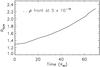 |
Fig. 8 Position of density front in terms of radial distance and time. |
The initial dynamics of the erupting flux rope is solely determined by the magnetic field as there are initially no pressure gradients. Once the eruption is under way, the key effect of the pressure gradient is to act as a counter force to the motion of the flux rope, through compression ahead and decompression behind. However, as long as the ejection of the flux rope takes place in a low β regime, the pressure gradients are not able to counter the dynamics. This does however mean that, the initial background configuration can have a significant impact on whether or not the ejection hits the outer boundary at 2.5 R⊙. An eruption which hits 2.5 R⊙ always takes place as long as the density front can move into an environment where β < 1. Thus the initial position of the β = 1 surface determines whether or not the eruption will be a full eruption, or a quenched one. We have performed additional simulations with a background pressure ten times larger than presented in the simulation here. It clearly shows that the eruption stops as soon as the flux rope travels out of the low-β region surrounding the bipoles. This is illustrated in Fig. 9 where we show maps of density with magnetic field lines superimposed along with the β = 1 contour. The state of the system is shown at the initial and final times: t = 0 τAlf and t = 69.6 τAlf. Although the initial magnetic field of the simulations are identical, as the background thermal pressure is ten times higher, the contour at β = 1 is lower in the atmosphere and now lies within the high density region. The flux rope and the dense plasma are ejected as before in the initial stages but now they reach a height of 1.6 R⊙ after t = 40 τAlf where the ejection is quenched. With the higher background pressure the rise of the flux rope is slower and it stops once the dense structure crosses over the β = 1 zone. This shows that the thermal pressure is critical in determining whether a full or quenched eruption takes place.
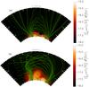 |
Fig. 9 Simulation with higher thermal pressure (p = 0.06). In a) and b) maps of log 10(ρ) on the (φ,r) plane passing through the centre of the bipoles at different times are shown. Superimposed are magnetic field lines plotted from the same starting points (green lines) and the contour line of β = 1 (white line). |
Finally, in order to check the validity of our simulation where we do not apply any external boundary driving we plot the variation of total energy in the domain as function of time in units of the initial total energy. The total energy is computed as the integral over the whole domain of the total energy, e which includes thermal, magnetic and kinetic energy. We show in Fig. 10 that the total energy is conserved over the simulation and as a result the eruption is not driven and is only due to forces present in the initial condition. At the end of the simulation approximately ~1% of the energy is lost, but this can be attributed to the open boundary conditions imposed at 2.5 R⊙ which allows energy to escape the domain.
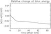 |
Fig. 10 Plot of the variation of total energy integrated in the whole domain as function on time in units of the initial total energy. |
4. Discussion
In the work presented here we have followed the full life span of a flux rope from formation to eruption. In doing so we have developed a new technique for coupling distinct forms of simulations, where the slow formation of the flux rope is modelled by a quasi-static approximation (Mackay & van Ballegooijen 2006a) and the eruption through a full MHD simulation. We now discuss a number of issues that have arisen in the present simulations and will be considered in future studies.
4.1. Magnetic configuration of the system
In our simulation, the flux rope forms and exists in a smoothly varying continuous magnetic configuration produced as a result of photospheric motions and flux cancellation. Within the magnetic field configuration the stress and forces applied have also been developed in a consistent way as may occur on the Sun. In the immediate surroundings above the flux rope there is the bipolar arcade and above this there is a large scale external arcade. The orientation of the magnetic field lines in the arcade are similar to that of the flux rope. This means that to some extend, the magnetic configuration is unfavorable for an ejection to escape.
4.2. Do we model the generation of a CME?
In the early stages the flux rope is initially ejected outwards as a single structure and it is possible to clearly follow its evolution. Within the flux rope trapped plasma is expelled and can be clearly identified. However, as soon as the flux rope moves beyond the symmetrical overlying arcade of the LHS bipole the dynamics become significantly more complex due to the interaction of the flux rope with the external magnetic field. After magnetic reconnection occurs high up it is no longer possible to clearly identify the flux rope. However, once the flux rope is no longer clearly identified the plasma does maintain its upward motion. Through following a dense front of plasma it reaches the top of our domain at 2.5 R⊙ travelling at a speed of around 100 km s-1. While such height reached by the dense front is promising for producing a CME, more investigations need to be performed to unambiguously answer the question as to whether or not we have modelled the generation of a CME.
In our simulation the characteristic three-component structure of CMEs is only hinted at, as we have just an indication of dense and void regions, but not the typical light-bulb shape. However this shape as seen in LASCO images is normally seen at radii much larger than that considered in the present simulations. This may also be partly due to the fact that the flux rope exists in a smoothly varying continuous magnetic field configuration and there is not a distinct flux rope cavity in the overlying magnetic field. Although the velocity of the expelled front is enough to let the plasma reach 2.5 R⊙ it only matches the slowest tail of the CME population. Nevertheless, with this initial study, based on an initial condition produced by slow quasi-static build up of stress using observed motion on the Sun, we have successfully modelled a plausible ejection for a CME.
4.3. What initiates the ejection?
The Lorentz force is the only force that exists in the initial condition, and it determines the initial evolution of the system. The initial condition of our simulation is in non-equilibrium and the radial component of the Lorentz force underneath and in the newly formed flux rope pushes it upwards. This force is a result of the formation of the flux rope such that it is too large to be held down by the overlying arcade. Therefore, the initial evolution and ejection of the flux rope is intrinsic to its existence in this scenario.
However, more complex dynamics occur later on in the simulation, when magnetic reconnection dominates the evolution of the flux rope. It occurs in two ways. First, the upward motion of the flux rope is enhanced by reconnection of magnetic field lines underneath the flux rope as it rises. Secondly, the magnetic field lines of the flux rope reconnect with the overlying open and closed magnetic field lines. This does not influence the onset of the dynamics of the ejection, but it is relevant for the geometry and shape of the ejection at later stages.
In summary, in the simulation there are different locations of reconnection. However magnetic reconnection only plays a major role for the ejection after the onset of the rise has occurred. Magnetic reconnection does not initiate the ejection, which starts because of a situation of non-equilibrium after the formation of the flux rope.
4.4. Is the role of thermal pressure important?
In the simulation, the thermal pressure is initially uniform. Though simple to implement it is not realistic for the solar corona. We however choose this as it does not add any additional forces in the gravity-less model. Within the presented simulation the key effect of the thermal pressure is to oppose the motion of the flux rope, through compression in front and rarefactions behind the flux rope. However, despite of the opposition from the thermal pressure the flux rope still reaches a height of 2.5 R⊙. Additional simulations show that if the background pressure is increased to be 10 times larger then the eruption is quenched in the corona.
An important aspect to consider is that our simulation does not include gravity. The gravitational force exerted on the plasma may prevent it and the flux rope from escaping from the sun. If we assume a stratified atmosphere in the initial conditions, the gravity force would be initially balanced by an upward directed pressure gradient. If we model the gravity in a properly stratified atmosphere, the confining power of the gravity might be negated by the upward directed pressure gradient. Additional simulations show that in the majority of cases gravity does not prevent the ejection, but only slows down the ejection. These results will be the subject of a future paper.
4.5. Differences with the GNLFFF model
Our work aims to bridge two different phases of the flux rope life span: the built up and the ejection. It starts from day 19 of the GNLFFF model after the flux rope has formed. Our MHD simulation then models the eruption of the flux rope over a period of a few hours after its construction and the onset of non-equilibrium.
In the simulations of Mackay & van Ballegooijen (2006a) after day 19, the flux rope also starts to rise in the corona. However it only reaches the higher corona after a number of days as the GNLFFF model is designed to damp evolution. In contrast the MHD code presented here properly describes the dynamic evolution of the system as it departs from the initial condition: in the presented simulation the ejection of the flux rope is complete in slightly more than two hours.
An important aspect of the simulations is that during the ejection above the LHS bipole the RHS bipole does not change significantly. Therefore if the erupting coronal magnetic field were to be allowed to settle back down to a force-free equilibrium, a slow quasi-static evolution could then be considered once again to follow the formation of a second flux rope above the RHS bipole. In future we will consider taking the post-eruption relaxed MHD state and inserting it back into the GNLFFF model to determine if another eruption can be produced at a different location.
An alternative approach to that considered here is to couple the GNLFFF with the MHD simulation at an earlier stage of the evolution, before the flux rope is fully formed. Then, by applying evolving boundary conditions in the MHD simulation identical to the ones of the GNLFF, the formation of the flux rope may be followed in the MHD framework. However, such attempt answers different questions than those addressed in the present paper and poses significant computational problems, relating to flux cancellation boundary condition in the MHD code and computational requirements.
5. Conclusions
In the work presented here, we investigate whether a flux rope slowly formed as result of flux cancellation and photospheric shearing motions in a smoothly varying continuous magnetic field distribution can lead to a fast ejection of plasma from the solar corona. In order to consider the full life span of the flux rope, we have coupled two models: the first is a GNLFFF model that describes the quasi-static formation of the flux rope over time periods of days to weeks and the second is a full MHD simulation that follows the evolution of the system once the flux rope is formed and becomes unstable. In our model no additional shearing or stress of the magnetic field is carried out in the MHD simulation, where the resulting dynamics are solely a result of the stress built up between the two bipoles during the slow evolution.
In our simulation the flux rope initially rises and then interacts with the overlying magnetic field resulting in significant magnetic reconnection above and below. The coronal plasma follows the magnetic field evolution and is expelled out to 2.5 R⊙. During this process the flux rope is deformed, so in future studies we need to investigate how the flux rope can conserve its shape during the eruption and how the plasma can be further accelerated, since the stress currently accumulated in the GNLFFF model is only enough to produce a modest ejection.
In many descriptions of the onset of CMEs, magnetic reconnection is used to produce the flux rope in a configuration ready to erupt (e.g. Aulanier et al. 2010) and we agree with this vision. In our scenario magnetic reconnection is used to produce the flux rope, but is not necessary in the early stages of the ejection. which is caused by a non-equilibrium. This is significantly different from other scenarios where magnetic reconnection does not play any role, like the Torus instability mechanism (which does not account for the flux rope formation).
We now discuss the role of thermal pressure in the modelling of our eruption. The thermal pressure plays no role in the initiation of the flux rope ejection, but can play a role in the propagation phase. In the present paper we have used a simple atmosphere as we focus more on the coupling of the two models rather than on the atmosphere profile. It is however important to include the role of thermal pressure if we want to move towards a realistic model of a solar eruption from generation to propagation into the interplanetary space. In the present simulations, thermal pressure inhibits the propagation of the flux rope and can quench the ejection in some scenarios (e.g. it obstructs the development of Torus instability Kliem & Török 2006). However, if the thermal pressure decays with height as in a stratified atmosphere its inhibition effect can be neglected. Therefore we will further investigate the effect of thermal pressure and of the atmospheric profile in future studies through included gravity in our model.
Another aspect of this study is to analyse additional magnetic configurations which have been subjected to the accumulation of more stress. In the GNLFFF model a flux rope can grow beyond the size of the flux rope described here. If the eruption is not released, the foot point motion and the flux cancellation can build up a stronger force underneath and the flux rope may then be expelled more violently.
An important achievement of the present work is the development of a technique that successfully couples two different models of the solar corona evolution. We develop such a technique because many different solar phenomena evolve over drastically different time scales. It is currently not possible to consider the full life span of flux ropes produced out of observed surface motions with only one model as computing power is currently insufficient to describe the formation and the ejection processes. In such a framework our efforts allow us to adopt the distinct models, i.e. different assumptions and approximations, during different stages of the coronal active region evolution. This opens up the possibility of many future studies of the Sun’s global magnetic field evolution which would not be possible otherwise.
Online material
Movie of Fig.7ad (GIF 3.50 MB) Access Supplementary Material
Movie of Fig.7eh (GIF 4.69 MB) Access Supplementary Material
Acknowledgments
D.H.M. would like to thank STFC, the Leverhulme Trust and the European Commission’s Seventh Framework Programme (FP7/2007−2013) for their financial support. P.P. would like to thank the European Commission’s Seventh Framework Programme (FP7/2007−2013) under grant agreement SWIFF (project 263340, www.swiff.eu) for financial support. These results were obtained in the framework of the projects GOA/2009-009 (KU Leuven), G.0729.11 (FWO-Vlaanderen) and C 90347 (ESA Prodex 9). The research leading to these results has also received funding from the European Commission’s Seventh Framework Programme (FP7/2007-2013) under the grant agreements SOLSPANET (project n 269299, www.solspanet.eu), SPACECAST (project n 262468, fp7-spacecast.eu), eHeroes (project n 284461, www.eheroes.eu). The computational work for this paper was carried out on the joint STFC and SFC (SRIF) funded cluster at the University of St Andrews (Scotland, UK).
References
- Amari, T., Luciani, J. F., Mikic, Z., & Linker, J. 2000, ApJ, 529, L49 [NASA ADS] [CrossRef] [PubMed] [Google Scholar]
- Amari, T., Luciani, J. F., Aly, J. J., Mikic, Z., & Linker, J. 2003, ApJ, 585, 1073 [NASA ADS] [CrossRef] [Google Scholar]
- Amari, T., Aly, J.-J., Luciani, J.-F., Mikic, Z., & Linker, J. 2011, ApJ, 742, L27 [NASA ADS] [CrossRef] [Google Scholar]
- Antiochos, S. K., DeVore, C. R., & Klimchuk, J. A. 1999, ApJ, 510, 485 [Google Scholar]
- Archontis, V., & Hood, A. W. 2008, ApJ, 674, L113 [NASA ADS] [CrossRef] [Google Scholar]
- Archontis, V., & Hood, A. W. 2012, A&A, 537, A62 [NASA ADS] [CrossRef] [EDP Sciences] [Google Scholar]
- Archontis, V., Hood, A. W., Savcheva, A., Golub, L., & Deluca, E. 2009, ApJ, 691, 1276 [Google Scholar]
- Aulanier, G., Démoulin, P., & Grappin, R. 2005, A&A, 430, 1067 [NASA ADS] [CrossRef] [EDP Sciences] [Google Scholar]
- Aulanier, G., Török, T., Démoulin, P., & DeLuca, E. E. 2010, ApJ, 708, 314 [Google Scholar]
- Chen, P. F. 2011, Liv. Rev. Sol. Phys., 8, 1 [Google Scholar]
- Cheng, X., Ding, M. D., & Zhang, J. 2010, ApJ, 712, 1302 [NASA ADS] [CrossRef] [Google Scholar]
- Cheng, X., Zhang, J., Liu, Y., & Ding, M. D. 2011, ApJ, 732, L25 [NASA ADS] [CrossRef] [Google Scholar]
- Fan, Y. 2009, ApJ, 697, 1529 [NASA ADS] [CrossRef] [Google Scholar]
- Fan, Y. 2010, ApJ, 719, 728 [NASA ADS] [CrossRef] [Google Scholar]
- Fan, Y., & Gibson, S. E. 2007, ApJ, 668, 1232 [Google Scholar]
- Forbes, T. G. 1991, Geophys. Astrophys. Fluid Dyn., 62, 15 [NASA ADS] [CrossRef] [Google Scholar]
- Forbes, T. G., & Isenberg, P. A. 1991, ApJ, 373, 294 [Google Scholar]
- Forbes, T. G., Linker, J. A., Chen, J., et al. 2006, Space Sci. Rev., 123, 251 [NASA ADS] [CrossRef] [Google Scholar]
- Hudson, H. S., Acton, L. W., Harvey, K. L., & McKenzie, D. E. 1999, ApJ, 513, L83 [NASA ADS] [CrossRef] [Google Scholar]
- Keppens, R., Meliani, Z., van Marle, A. J., et al. 2012, J. Comput. Phys., 231, 718 [Google Scholar]
- Kliem, B., & Török, T. 2006, Phys. Rev. Lett., 96, 255002 [NASA ADS] [CrossRef] [PubMed] [Google Scholar]
- Liu, R., Liu, C., Wang, S., Deng, N., & Wang, H. 2010, ApJ, 725, L84 [NASA ADS] [CrossRef] [Google Scholar]
- Low, B. C. 1996, Sol. Phys., 167, 217 [Google Scholar]
- Lynch, B. J., Gruesbeck, J. R., Zurbuchen, T. H., & Antiochos, S. K. 2005, J. Geophys. Res. (Space Physics), 110, 8107 [NASA ADS] [CrossRef] [Google Scholar]
- Mackay, D. H., & van Ballegooijen, A. A. 2006a, ApJ, 641, 577 [NASA ADS] [CrossRef] [Google Scholar]
- Mackay, D. H., & van Ballegooijen, A. A. 2006b, ApJ, 642, 1193 [NASA ADS] [CrossRef] [Google Scholar]
- Mackay, D. H., Karpen, J. T., Ballester, J. L., Schmieder, B., & Aulanier, G. 2010, Space Sci. Rev., 151, 333 [NASA ADS] [CrossRef] [Google Scholar]
- Manchester, IV, W., Gombosi, T., DeZeeuw, D., & Fan, Y. 2004, ApJ, 610, 588 [NASA ADS] [CrossRef] [Google Scholar]
- McKenzie, D. E., & Canfield, R. C. 2008, A&A, 481, L65 [NASA ADS] [CrossRef] [EDP Sciences] [Google Scholar]
- Powell, K. G., Roe, P. L., Linde, T. J., Gombosi, T. I., & de Zeeuw, D. L. 1999, J. Comput. Phys., 154, 284 [NASA ADS] [CrossRef] [Google Scholar]
- Reeves, K. K., Linker, J. A., Mikić, Z., & Forbes, T. G. 2010, ApJ, 721, 1547 [NASA ADS] [CrossRef] [Google Scholar]
- Roussev, I. I., Galsgaard, K., Downs, C., et al. 2012, Nat. Phys., 8, 845 [NASA ADS] [CrossRef] [Google Scholar]
- Savcheva, A., Pariat, E., van Ballegooijen, A., Aulanier, G., & DeLuca, E. 2012, ApJ, 750, 15 [NASA ADS] [CrossRef] [Google Scholar]
- Schwenn, R. 2006, Space Sci. Rev., 124, 51 [NASA ADS] [CrossRef] [Google Scholar]
- Török, T., & Kliem, B. 2005, ApJ, 630, L97 [Google Scholar]
- Török, T., & Kliem, B. 2007, Astron. Nachr., 328, 743 [NASA ADS] [CrossRef] [Google Scholar]
- Tóth, G., & Odstrcil, D. 1996, J. Comput. Phys., 128, 82 [Google Scholar]
- van Ballegooijen, A. A., & Martens, P. C. H. 1989, ApJ, 343, 971 [NASA ADS] [CrossRef] [Google Scholar]
- Wood, B. E., Karovska, M., Chen, J., et al. 1999, ApJ, 512, 484 [Google Scholar]
- Yeates, A. R., & Mackay, D. H. 2009, ApJ, 699, 1024 [Google Scholar]
- Yeates, A. R., Attrill, G. D. R., Nandy, D., et al. 2010, ApJ, 709, 1238 [NASA ADS] [CrossRef] [Google Scholar]
Appendix A: Interpolation of B from the GNLFFF code to ARMVAC
To import B from the GNLFFF model to the MHD code, we perform a 3D second order interpolation in spherical coordinates. In Fig. A.1 we see an illustration of the r-φ plane on a flat surface. The black grid, represents the GNLFFF grid, where individual magnetic field components (BGNLFFF) are defined at cell ribs. The red grid represents the MHD grid, where all components of BVAC are defined at the cell centres. The two grids have a different number of points and different spacing: the GNLFFF grid is composed of 106 × 172 × 181 cells, where the cell size is non-uniform (see Mackay & van Ballegooijen 2006a). In contrast the AMRVAC grid is composed of 132 × 128 × 128 cells uniformly spaced. As the black and red cells in Fig. A.1 are of a different size they do not directly match. Due to this, the relative position and values of the components of BGNLFFF and BVAC cannot be determined by simple symmetry conditions. To interpolate from the GNLFFF code to the MHD code, we identify the cell of the GNLFFF grid into which each point of the MHD grid falls. We then use the values of the adjacent GNLFFF cells for the computation of the interpolated magnetic field:
![Mathematical equation: \appendix \setcounter{section}{1} \begin{eqnarray} \label{interpolation} &&\vec{B}^{\rm VAC}_{[r,\theta,\phi]}(k_r,j_{\theta},i_{\phi})=\vec{B}^{\rm GNLFFF}_{[r,\theta,\phi]}(r_0,\theta_0,\phi_0)\notag\\&&+ \nabla\vec{B}^{\rm GNLFFF}_{[r,\theta,\phi]}\cdot\vec{\Delta s} +\frac{1}{2}|{\bf H^{\rm GNLFFF}(\vec{r}_0,\theta_0,\phi_0)}|\vec{\Delta s}^2 \end{eqnarray}](/articles/aa/full_html/2013/06/aa20947-12/aa20947-12-eq94.png) (A.1)where kr,jθ,iφ are the indexes identifying the position in the MHD grid and
(A.1)where kr,jθ,iφ are the indexes identifying the position in the MHD grid and ![Mathematical equation: \hbox{$\vec{B}^{\rm GNLFFF}_{[r,\theta,\phi]}(r_0,\theta_0,\phi_0)$}](/articles/aa/full_html/2013/06/aa20947-12/aa20947-12-eq98.png) are the values of the components of BGNLFFF closest to the coordinates of the point (kr,jθ,iφ) and Δs = (dr,rdθ,rsinθdφ). The adjacent cells are used to compute the gradients of the components of the magnetic field,
are the values of the components of BGNLFFF closest to the coordinates of the point (kr,jθ,iφ) and Δs = (dr,rdθ,rsinθdφ). The adjacent cells are used to compute the gradients of the components of the magnetic field, ![Mathematical equation: \hbox{$\nabla\vec{B}^{\rm GNLFFF}_{[r,\theta,\phi]}$}](/articles/aa/full_html/2013/06/aa20947-12/aa20947-12-eq100.png) and the Hessian matrix | HGNLFFF(r0,θ0,φ0) | through finite differences. The second order interpolation is performed as it guarantees a correct transporting of the spatial derivatives of B between the codes and thus the Lorentz Force.
and the Hessian matrix | HGNLFFF(r0,θ0,φ0) | through finite differences. The second order interpolation is performed as it guarantees a correct transporting of the spatial derivatives of B between the codes and thus the Lorentz Force.
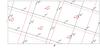 |
Fig. A.1 Illustration of a portion of the r-φ plane onto a flat surface where we sketch the two grids. Black lines represent the GNLFFF code: the magnetic field components are defined on different ribs of the cells. Red lines represent the cells of AMRVAC: all the magnetic field components are defined in the centre of the cell. |
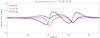 |
Fig. A.2 Comparison of the components of B in the GNLFFF model (continuous lines) and in the MHD model (crosses) after interpolation. |
In Fig. A.2 we compare the three components of B in the GNLFFF model and the MHD code along the φ direction for a typical case. The profiles of each component of the magnetic field in the GNLFFF model (continuous lines) and the magnetic field interpolated in the MHD code (crosses) match well. At the lower boundary, where the gradients of the magnetic field components are the steepest, the interpolated magnetic field departs by at most 1% from the original magnetic field.
Appendix B: Equilibrium test
To check the validity of our approach, before we consider an erupting system we perform a test where a magnetic field configuration in force balance (i.e. (∇ × B) × B = 0) is transported from the GNLFFF model into ARMVAC. Through this we verify that the Lorentz force is properly transported between the codes and that the MHD numerical modelling does not generate artificial forces. This test is performed using an initial condition similar to the case we wish to investigate, consisting of two magnetic bipoles that lie close to one-other but are not overlapping (see Figs. B.2a and b). The magnetic field configuration used is a potential magnetic feld computed from the photospheric magnetic field at Day 21 in Mackay & van Ballegooijen (2006a). The B0 magnetic field is also a potential magnetic field but computed from the photospheric magnetic field at Day 19. Therefore, in such set up, although both B and B0 are potential magnetic fields, they are not identical, as they correspond to a different photosphetic magnetic field. This results in a non-zero B1 that is allowed to evolve in time, according to the MHD equations presented in Sect. 2.3.
As the magnetic field is potential, we expect this configuration to be in stable equilibrium and we should not observe any significant departure from the initial distribution of magnetic field, density, and pressure. Also the assumptions we make about the spatial distribution of ρ and p should not introduce any dynamics. Our assumption in Eq. (1) and the typical values of parameters we use lead to a uniform Alfven speed of ~108 cm/s at t = 0 s. With these parameters we obtain an atmospheric profile in the radial direction for the density and plasma beta, β = 8πp/B2 taken from the centre point of the bipoles, as shown in Fig. B.1. The plasma beta varies from 10-3 at the photosphere to over 103 at the top of the box, while the coronal density drops by over five orders of magnitude.
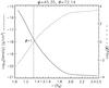 |
Fig. B.1 Profile of log 10(ρ) and log 10(β) along r at fixed colatitude and longitude in our typical simulation. The vertical dotted line shows the height of β = 1. |
With these values the Alfvén crossing time, i.e. the time for an Alfvén wave to travel from one side of the domain to the other, is about 1000 s. While this is one of the time scales that can be determined, for our study a better time scale is the time it takes an Alfvén wave to travel across a single bipole. This Alfvén travel time is around τAlf = 120 s so we define this as the characteristic time in the simulation.
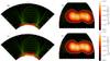 |
Fig. B.2 Illustration of the evolution of magnetic field and plasma in the test simulation with a potential field. a) and c) maps of log 10(ρ [g/cm3]) in the (r,φ) plane passing through the centre of the bipoles (at t = 0 τAlf, and at t = 142.10 τAlf). b) and d) same maps at the r = 1.09 R⊙ surface. Superimposed are magnetic field lines plotted from the same starting points (green lines) and the contour line of β = 1 (white line). |
In order to test the stability of the system we let the system evolve for a large number of Alfvén times. Figure B.2 shows the initial configuration of the magnetic field at t = 0 (Figs. B.2a and b) and after t ~ 140 τAlf (Figs. B.2c and d), where the green lines represent magnetic field lines plotted from the same starting point at both times. Over the 80 Alfvén times, the magnetic field does not show any significant evolution. At the end of the simulation, changes to the magnetic field are of the order of 1% of the initial value. Thus importing the magnetic field from the GNLFFF code has not generated any additional forces.
Note that the plasma density distribution does not show any signifcation evolution, even though small scale changes occur. At most, the bulk velocity is of the order of 104 cm/s, but only appear in regions external to the bipoles, where the density is very low. This shows that the transporting between the GNLFFF and MHD models is possible and that the coupling of the two codes is physically consistent and free from numerical artefacts.
All Figures
|
Fig. 1 Configuration of the magnetic field after 19 days of evolution using the model of Mackay & van Ballegooijen (2006a). The figure shows a sample of magnetic field lines that illustrate the structure of the magnetic bipoles, the overlying arcade, and the newly formed magnetic flux rope along the PIL of the left-hand side bipole. The surface boundary is coloured according to the polarity of the magnetic field: negative polarity is black and positive is white. |
| In the text | |
|
Fig. 2 Illustration of the coupling of the GNLFFF variables as input for the MHD code. We interpolate the magnetic field B of the GNLFFF model for use in the MHD code. From B we then deduce the density. The velocity is then automatically created in the MHD code and thermal pressure set. |
| In the text | |
|
Fig. 3 Magnetic field configuration used as the initial condition in the MHD simulations of the erupting flux rope. Red lines represent the flux rope, blue lines the arcades, green lines the external magnetic field. The lower boundary is coloured according to the intensity of the magnetic field from red (strong) to blue (weak) in arbitrary units. |
| In the text | |
|
Fig. 4 Radial component of the Lorentz Force on the r − φ plane at the centre of the bipole at a) t = 0 τAlf and b) t = 23.20 τAlf. In panel b) the dashed black lines mark the contours of negative radial component of the Lorentz force at FLR = −2 × 10-11 dyne. Red lines represent some magnetic field lines. |
| In the text | |
|
Fig. 5 Magnetic field lines departing from the same points of the LHS bipole polarity regions at a) t = 2.61 τAlf and b) t = 2.67 τAlf. |
| In the text | |
|
Fig. 6 a) Radial component of the velocity on the r − φ plane through the centre of the bipole at t = 11.6 τAlf. b) Radial component of the velocity on the θ − φ plane at r = 1.07 R⊙ at the same time with superimposed contours of the radial component of the magnetic field (black lines, dashed lines for negative values and solid lines for positive values) and the projection of the horizontal velocity field onto the same θ − φ plane (green arrows, typical velocity is 2 × 106 cm/s and minimum velocity shown is 1.3 × 106 cm/s). |
| In the text | |
|
Fig. 7 a)−d) Maps of log 10(ρ) on the (φ,r) plane passing through the centre of the bipoles at different times. Super-imposed are magnetic field lines plotted from the same points (green lines) and a contour line at β = 1 (white line). e)−h) Magnetic configurations at the same times as the LHS column. Yellow magnetic field lines depart from the negative polarity of the LHS bipole, blue magnetic lines depart from the positive polarity of the LHS bipole, green magnetic lines represent the external magnetic field. All the magnetic field lines in panels a)−d) and e)−h) are plotted from the same starting points at all the times. |
| In the text | |
|
Fig. 8 Position of density front in terms of radial distance and time. |
| In the text | |
|
Fig. 9 Simulation with higher thermal pressure (p = 0.06). In a) and b) maps of log 10(ρ) on the (φ,r) plane passing through the centre of the bipoles at different times are shown. Superimposed are magnetic field lines plotted from the same starting points (green lines) and the contour line of β = 1 (white line). |
| In the text | |
|
Fig. 10 Plot of the variation of total energy integrated in the whole domain as function on time in units of the initial total energy. |
| In the text | |
|
Fig. A.1 Illustration of a portion of the r-φ plane onto a flat surface where we sketch the two grids. Black lines represent the GNLFFF code: the magnetic field components are defined on different ribs of the cells. Red lines represent the cells of AMRVAC: all the magnetic field components are defined in the centre of the cell. |
| In the text | |
|
Fig. A.2 Comparison of the components of B in the GNLFFF model (continuous lines) and in the MHD model (crosses) after interpolation. |
| In the text | |
|
Fig. B.1 Profile of log 10(ρ) and log 10(β) along r at fixed colatitude and longitude in our typical simulation. The vertical dotted line shows the height of β = 1. |
| In the text | |
|
Fig. B.2 Illustration of the evolution of magnetic field and plasma in the test simulation with a potential field. a) and c) maps of log 10(ρ [g/cm3]) in the (r,φ) plane passing through the centre of the bipoles (at t = 0 τAlf, and at t = 142.10 τAlf). b) and d) same maps at the r = 1.09 R⊙ surface. Superimposed are magnetic field lines plotted from the same starting points (green lines) and the contour line of β = 1 (white line). |
| In the text | |
Current usage metrics show cumulative count of Article Views (full-text article views including HTML views, PDF and ePub downloads, according to the available data) and Abstracts Views on Vision4Press platform.
Data correspond to usage on the plateform after 2015. The current usage metrics is available 48-96 hours after online publication and is updated daily on week days.
Initial download of the metrics may take a while.