| Issue |
A&A
Volume 553, May 2013
|
|
|---|---|---|
| Article Number | L4 | |
| Number of page(s) | 10 | |
| Section | Letters | |
| DOI | https://doi.org/10.1051/0004-6361/201321382 | |
| Published online | 01 May 2013 | |
WMAP nine-year CMB estimation using sparsity ⋆
Laboratoire AIM, UMR CEA–CNRS–Paris 7, Irfu, SAp/SEDI, Service d’Astrophysique, CEA Saclay, 91191 Gif-sur-Yvette Cedex, France
e-mail: jerome.bobin@cea.fr
Received: 28 February 2013
Accepted: 22 March 2013
Recovering the cosmic microwave background (CMB) from WMAP data requires that Galactic foreground emissions are accurately separated out. Most component separation techniques rely on second-order statistics such as internal linear combination (ILC) techniques. We present a new WMAP nine-year CMB map with a resolution of 15 arcmin, which is reconstructed using a recently introduced sparse-component separation technique, called local generalized morphological component analysis (LGMCA). This focuses on the sparsity of the components to be retrieved in the wavelet domain. We show that although they are derived from a radically different separation criterion (i.e. sparsity), the LGMCA-WMAP 9 map and its power spectrum are fully consistent with their more recent estimates from WMAP 9.
Key words: methods: data analysis / cosmic background radiation / methods: statistical
Appendices A–C are available in electronic form at http://www.aanda.org
© ESO, 2013
1. Introduction
The cosmic microwave background (CMB) is a snapshot of the state of the Universe at the time of recombination. It provides information about the primordial Universe and its evolution to the current state. Our current understanding of our Universe is heavily based on measurements of the CMB radiation. The statistical properties of CMB fluctuations depend on the primordial perturbations from which they arose as well as on the subsequent evolution of the Universe as a whole. For cosmological models in which initial perturbations are of a Gaussian nature, the information carried by CMB anisotropies can completely be characterized by their angular power spectrum, which depends on the cosmological parameters. This makes the precise measurement of the CMB power spectrum a gold mine for understanding and describing the Universe throughout its history.
In estimating the CMB map, the astrophysical foreground emissions from our galaxy and the extraGalactic sources have to be removed. In addition, the instrumental noise hinders estimating the CMB map. In the low frequency regime (below 100 GHz, i.e. for WMAP channels) the strongest contamination comes from the Galactic synchrotron and free-free emission, with the highest contribution at large angular scales. At higher frequencies, dust emissions dominate, whereas the synchrotron and free-free emissions are low. The spinning dust is an extra emission that spatially correlates with dust and dominates at low frequencies.
Since second-order statistics provide sufficient statistics for a Gaussian CMB field, most of the component separation techniques, such as the internal linear combination (ILC), are built upon them to recover the CMB map from the observed sky maps. However, these techniques are not ideal for non-stationary and non-Gaussian components such as the foregrounds (or even non-stationary noise). In contrast, sparsity-based source-separation techniques that focus on the higher-order statistics of the components have proven to be highly efficient (Bobin et al. 2007, 2013).
In this paper, we present a new WMAP nine-year CMB estimation based on this sparsity concept and compare the results to the official WMAP products. Section 2 briefly describes the local generalized morphological component analysis (LGMCA) method. We then describe in Sect. 3 the processing of WMAP data, and the derived LGMCA products are displayed in Sect. 4. The results of WMAP simulations are presented in Appendix C.
2. Component separation for CMB maps
Exploiting the fact that foreground components are sparse in the wavelet domain (i.e., a few wavelet coefficients are enough to represent most of the energy of the component), LGMCA (Bobin et al. 2013) estimates the components of interest and the mixing matrix by maximizing the sparsity level of each component; it seeks the sparsest sources possible on a wavelet basis. The assumption is that the observed sky is a linear combination of all components, each resulting from a completely different physical process, and the instrumental noise. The separation principle in this method relies on the different spatial morphologies or structures of the various foregrounds, which translate into different sparsity patterns when transformed to a fixed wavelet dictionary. A linear combination of these components decreases the level of sparsity. Therefore, reconstructing each component from the observed map by maximizing its sparsity level in wavelet space is an efficient strategy to distinguish between physically different sources. As mentioned in Appendix A, channel resolution variation and spatial variations of component emissions such as dust are taken into account by estimating a mixing matrix per wavelet scale and per area. Full details are given in Bobin et al. (2013).
In Appendix C, the LGMCA is evaluated on simulated WMAP data and we found the following:
-
The recovered power spectrum from the LGMCA map at 15 arcmin is within the 2σ error bars from the input CMB power spectrum.
-
The propagated noise in the map is the main residual contamination for the LGMCA; for low multipoles, the contaminants are much lower than the cosmic variance.
-
Compared to a pixel-based localized ILC computed at 1 degree, both noise and foregrounds residuals are lower using the LGMCA.
-
No significant non-Gaussianities at various scales and positions are detected in the LGMCA maps, either at 1 degree or 15 arcmin. Compared to the pixel-based localized ILC, no significant difference is observed for LGMCA at 1 degree compared to the errors expected.
In combination, these results are an incentive to apply the LGMCA to WMAP9 data.
3. Map and power spectrum estimation
The WMAP satellite has observed the sky in five frequency bands denoted K, Ka, Q, V, and W centered on 23, 33, 41, 61, and 94 GHz. The released data include sky maps obtained with ten differencing assemblies for nine individual years; per year, there is one map for the K band and one for the Ka band, two for the Q band, two for the V band and four for the W band. These maps are sampled using the HEALPix pixelization scheme at a resolution corresponding to nside of 1024. At first, we averaged all differencing-assembly maps obtained for the same frequency band, which yields five band-averaged maps. However, these maps are not offset-corrected. To determine the offset value for a particular frequency band, we used the standard resolution of the nine-year band-average maps of WMAP as reference maps. Offset values were obtained by determining the mean of the difference between the band-averaged map being considered and the reference map.
At the WMAP frequencies, the major sources of contamination in the maps are the synchrotron, free-free, spinning dust, and thermal dust. To model the foreground contamination, we used two foreground templates in our analysis: dust at 100 microns, as obtained by (Schlegel et al. 1998) and the composite all-sky H-alpha map of (Finkbeiner 2003). Among these templates, the thermal dust template is the most important one, as it helps in removing the dust emission on small scales, which is otherwise significant in the W channel. Because the spinning dust is spatially correlated with thermal dust, the thermal dust template also helps in reducing the spinning dust residuals. It is standard to use the 408 MHz synchrotron map of (Haslam et al. 1981) as a template for the synchrotron emission. However, this map has a quite resolution of about 1 degree. Furthermore, adding this template to the LGMCA did not improve the component separation.
LGMCA map: following (Bobin et al. 2013), the LGMCA was applied to the five offset-corrected WMAP maps and the two templates used as extra observations. Details on the LGMCA parameters are given in Appendix B.
LGMCA power spectrum: using the mixing matrices previously estimated from all data, we can estimate a CMB map from each of the nine individual year data sets. From these nine maps, we derived all 36 possible cross-spectra using thehigh-resolution temperature analysis mask kq85 with (fsky = 0.75)1 provided by WMAP collaboration. The final CMB power spectrum is then obtained by averaging them and using a MASTER mask deconvolution (Hivon et al. 2002). In contrast to the CMB and foreground signals, noise is uncorrelated between different years of data and is therefore considerably reduced in the averaged cross spectrum.
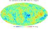 |
Fig. 1 ILC official WMAP nine year map (1 degree resolution). Units in μK. |
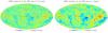 |
Fig. 2 Estimated LGMCA CMB map from WMAP (nine years) at 15 arcmin resolution and 1 degree. Units in μK. |
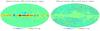 |
Fig. 3 Difference between the estimated CMB map with LGMCA and the official ILC map. The bottom panel shows the same difference map masked with the kq85 mask. |
4. Results
LGMCA map and power spectrum
Figure 1 shows the official ILC WMAP nine years CMB map, which has a 1 degree resolution, and Fig. 2 shows the LGMCA WMAP CMB map at 15 arcmin resolution and at 1 degree. The 15 arcmin LGMCA map exhibits slight high-frequency structures, which are most likely related to point source emission from the Galactic center. The two 1-degree maps look very clean, even on the Galactic center. Figure 3 features the difference at 1 degree resolution between the CMB map estimated with the LGMCA and the official ILC-based CMB map provided by the WMAP consortium. The difference map shows significant foreground residuals at the Galactic center, which are roughly three times lower than the CMB level however. When masking the Galactic center with the kq85 WMAP mask (Fsky = 75%), no significant feature can be seen anymore.
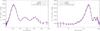 |
Fig. 4 Estimated CMB map power spectrum from WMAP (nine years) in linear scale (top panel) and logarithmic scale (bottom panel). Units in μK2. |
The estimated power spectrum is displayed in Fig. 4. The error bars, essentially the cosmic variance and the noise-related variance, were derived from classical power spectrum variance estimators as described in (Greason et al. 2013). Note that except for ℓ < 32, the official WMAP nine year power spectrum (in blue in Fig. 4) was computed from the V and W bands only. In contrast, the spectrum in red in Fig. 4 was derived from the full dataset. Even if the estimation procedure differs slightly, it is remarkable that the two power spectra look very similar. They also tend to depart from each other with a slightly lower third multipole. Furthermore, the measurement of the third peak seems to be higher to some extent. However, the two spectra are compatible at all scales within 2σ error bars.
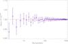 |
Fig. 5 Mean ratio of |
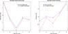 |
Fig. 6 Comparison of skewness and kurtosis in ILC and LGMCA map at 1 degree computed for the various wavelet scales described in Fig. C.4 (left). The wavelet filters peak multipole 240, 120, 60, 30, and 15 for scales 1 to 5. |
Sanity check: the LGMCA algorithm computes mixture parameters (i.e., mixing matrices and their inverse) that were applied subsequently to the data to estimate the CMB map. It is important to note that the final CMB map linearly depends on the input data. This makes it possible to check whether the inversion process may induce some bias at the level of the estimated CMB map and its power spectrum (assuming no calibration or beam errors). For that purpose, we applied exactly the same parameters as we computed from the real data to 100 random CMB realizations. These realizations were generated as Gaussian random processes with a power spectrum defined by the WMAP nine-year best-fit theoretical power spectrum. The point spread function of these simulations were chosen as the beams of the nine-year band-average maps of WMAP, which provided pure CMB simulations that mimic the CMB part of the WMAP nine year data. Figure 5 shows in blue the ratio between the estimated and theoretical power spectrum  computed from an average of 100 random CMB simulations. The theoretical power spectrum
  of the simulated CMB maps is exactly defined as the WMAP nine year best-fit power spectrum. The error bars are defined as the cosmic variance from 100 simulations. If the estimation with the LGMCA of the CMB map and more specifically its power spectrum were biased, the would depart from 1. Figure 5 shows that there is no statistical evidence of discrepancy from 1. We therefore conclude that the LGMCA does not introduce any bias at the level of the CMB power spectrum.Any bias of the estimated CMB map will come from remaining noise and foreground contamination.
Higher order statistics — non-Gaussianities: higher order statistics were also computed for the full nine year CMB maps recovered at 1 degree with ILC and LGMCA to assess potential differences in their distribution. The 75% mask was employed on both maps to avoid computing the higher order statistics in regions contaminated by foreground residuals. Sparse inpainting was then performed to interpolate the signal inside the mask (Starck et al. 2013) to avoid artifacts on the wavelet coefficients, and the skewness and kurtosis were calculated for each wavelet scale considering only the wavelet coefficients within the mask. These statistics were centered and normalized by similarly processing a set of 100 realizations of noise and CMB according to the Λ-CDM fit provided by the WMAP consortium. Figure 6 shows the skewness and kurtosis versus the wavelet scale and illustrates that not only that the ILC and LGMCA maps are compatible with no non-Gaussianities, but also that no significant difference between ILC and LGMCA can be found with these statistics at that resolution.
5. Conclusion
We have investigated how sparsity could be used for a WMAP CMB map reconstruction. Based on WMAP simulations, we showed that the LGMCA provides a low-foreground map and that noise remains the main source of contamination. Then a high-resolution (15 arcmin) clean CMB map was computed from the full WMAP nine year dataset and its power spectrum was estimated. Remarkably, though the LGMCA-based and official WMAP nine year power spectrum were derived from completely different estimation procedures, they agree very well and are compatible within 2σ error bars. Lastly, non-Gaussianity tests based on higher order statistics were carried out, and showed no statistically significant departure from Gaussianity at a resolution of 1 degree. The LGMCA and the official WMAP 9 maps essentially differ close to the Galactic center where it remains extremely difficult to assess which map is less contaminated by foreground residuals or biases due to chance correlations in between CMB and foregrounds.
The LGMCA code is available at http://www.cosmostat.org/lgmca and the LGMCA CMB map as well as the estimated power spectrum are available at http://www.cosmostat.org/product.
Online material
Appendix A: The LGMCA method
The GMCA framework
The generalized morphological component analysis (GMCA) method is based on blind source separation (BSS, Bobin et al. 2013). In the framework of BSS, each of the five WMAP frequency channels are modeled as a linear combination of n components: 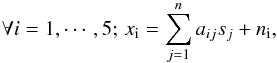 (A.1)where sj stands for the jth component, aij is a scalar that models the contribution of the jth component to channel i, and ni models the instrumental noise. This problem is more conveniently recast into the matrix formulation
  (A.2)In practice, the number of components is set to n = 5, which allows for more degrees of freedom to obtain a clean CMB map while keeping A invertible. In constrast to standard approaches in astrophysics (see Bobin et al. 2013, and references therein), the GMCA relies on the sparsity of the components S in the wavelet domain. Taking the data to the wavelet representation only alters the statistical distribution of the data coefficients without affecting its information content. A wavelet transform tends to grab the informative coherence between pixels while averaging the noise contributions, thus enhancing the structure in the data. This allows one to better distinguish components that do not share the same sparse distribution in the wavelet domain. In addition, sparsity has the ability to be more sensitive to non-Gaussian processes, which has been shown to improve the foreground separation method.
With A as the mixing matrix and Φ as a wavelet transform, we assume that each source sj can be sparsely represented in Φ; sj = αjΦ. The multichannel noiseless data Y can be written as  (A.3)where α is a Ns × T matrix whose rows are αj.
This means that the sparsity of the sources in Φ translates into sparsity of the multichannel data Y. The GMCA algorithm seeks an unmixing scheme through estimating A, which leads to the sparsest sources S. This is expressed by the following optimization problem (written in the augmented Lagrangian form) 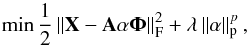 (A.4)where typically p = 0 (or its relaxed convex version with p = 1) and ∥X∥F = sqrt(trace(XTX)) is the Frobenius norm.
Local GMCA
The local-GMCA (LGMCA) algorithm (Bobin et al. 2013) has been introduced as an extension of GMCA:
-
multi-frequency instruments generally provide observationsthat do not share the same resolution. For example, the WMAPfrequency channels have a resolution that ranges from 13.2 arcmin for the W band to 52.8 arcmin for the K band. This makes the linear mixture model underlying the GMCA algorithm invalid. It is customary to alleviate this problem by degrading the frequency channels down to a common resolution prior to applying any component separation technique (the official CMB map provided by the WMAP consortium has a resolution of 1 degree). For this purpose, the data are decomposed in the wavelet domain, and at each wavelet scale we only use the observations with invertible beams and then degrade the maps to a common resolution. This allows us to estimate a CMB map with a resolution of 15 arcmin.
-
most foreground emissions (e.g. thermal dust, synchrotron, free-free) have electromagnetic spectra that are not spatially constant. In the framework of GMCA, this translates into a mixing matrix A that also varies across the pixels. Dealing with the variation across pixels of the electromagnetic spectrum of some of the components, the LGMCA estimates the mixing matrices on patches at various wavelet scales with band-dependent size.
The LGMCA algorithm has been implemented and evaluated on simulated Planck data in (Bobin et al. 2013).
Appendix B: LGMCA parameters for WMAP data
As described in Appendix A, LGMCA mixing matrices are estimated from a set of input channels at a given resolution on a patch of data at a given wavelet scale. For WMAP data, the parameters used by the LGMCA to compute these matrices are described in Table B.1. Figure B.1 displays the filters in spherical harmonics defining the wavelet bands at which the derived weights (by inverting these mixing matrices) were applied.
Parameters used in LGMCA to process the WMAP data with ancillary data.
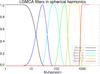 |
Fig. B.1 Filters defining the wavelet bands used in LGMCA. |
Appendix C: Simulations
In this section, the LGMCA algorithm is applied to data simulated by the Planck Sky Model (PSM) developed by Delabrouille and collaborators2 (Delabrouille et al. 2013). The PSM models the astrophysical foregrounds in the range of frequencies probed by WMAP, the simulated instrumental noise, and the beams. In detail, the simulations were obtained as follows.
-
Frequency channels: the simulated data comprised the 5 WMAP channels at frequency 23, 33, 41, 61, and 94 GHz. The frequency-dependent beams are perfectly isotropic PSFs; their profiles were obtained as the mean value of the beam transfer functions of at each frequency as provided by the WMAP consortium (nine years version).
-
Instrumental noise: instrumental noise was generated according to a Gaussian distribution with the covariance matrix provided by the WMAP consortium (nine years version).
-
Cosmic microwave background: the CMB map is a Gaussian random realization whose theoretical power spectrum is defined as the WMAP (nine years) best-fit power spectrum (from the six cosmological parameters model). The simulated CMB is perfectly Gaussian, and no non-Gaussianity (e.g. lensing, ISW, fNL) was added. This will allow for non-Gaussianity tests under the null assumption in the sequel.
-
Dust emissions: the Galactic dust emissions is composed of two distinct dust emissions: thermal dust and spinning dust (a.k.a. anomalous microwave emission). Thermal dust is modeled with the Finkbeiner model (Finkbeiner et al. 1999), which assumes that two hot/cold dust populations contribute to the signal in each pixel. The emission law of thermal dust varies across the sky.
-
Synchrotron emission: the synchrotron emission, as simulated by the PSM, is an extrapolation of the Haslam 408 MHz map (Haslam et al. 1982). The emission law of the synchrotron emission is an exact power law with a spatially varying spectral index.
-
Free-free emission: the spatial distribution of free-free emission is inspired by the Hα map built from the SHASSA and WHAM surveys. The emission law is a perfect power law with a fixed spectral index.
-
Point sources: infrared and radio sources were added based on existing catalogs at that time (including WMAP7 sources). In the following, the brightest point sources are masked prior to the evaluation results.
A simulated WMAP dataset was produced for each of the nine years. This allows to process the simulated data in the same manner as the WMAP data are processed.
Component separation
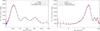 |
Fig. C.1 Estimated CMB map power spectrum from simulated WMAP (nine years). |
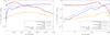 |
Fig. C.2 Estimated CMB map, noise, and remaining foreground power spectra from simulated WMAP (nine years) at 15 arcmin resolution. |
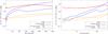 |
Fig. C.3 Comparisons between LGMCA and ILC at 1 degree resolution. Estimated CMB map, noise, and remaining foreground power spectra from simulated WMAP (nine years). Additionally, the amplitudes have been amplified by |

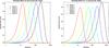 |
Fig. C.4 Legendre coefficients of the wavelet filters employed for non-Gaussianity analyses at 1 degree (left) and 15 arcmin (right). These wavelets are well localized in pixel space, allowing a fine analysis per latitude band. |
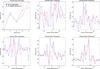 |
Fig. C.5 Comparison of skewness levels in the LGMCA (red) and ILC (blue) maps at 1 degree computed for various wavelet scales. These statistics were centered on the expected value and normalized from a set of 100 simulations of CMB and noise (see text). |
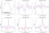 |
Fig. C.6 Comparison of centered and normalized kurtosis in the LGMCA (red) and ILC (blue) maps at 1 degree computed for various wavelet scales. The same mask and set of simulations where employed as in Fig. C.5. |
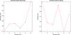 |
Fig. C.7 Centered and normalized skewness and kurtosis in the LGMCA map at 15 arcmin computed for various wavelet scales. A 75% mask and a set of 100 simulations of CMB and noise were used to compute these statistics (see text). |
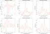 |
Fig. C.8 Centered and normalized skewness in the LGMCA map at 15 arcmin computed for various wavelet scales and locations. The same mask and set of simulations were employed to derive the statistic as in Fig. C.7. |
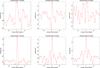 |
Fig. C.9 Centered and normalized kurtosis in the LGMCA map at 15 arcmin computed for various wavelet scales and locations. The same mask and set of simulations were employed the statistic as in Fig. C.7. |
The same templates and parameters as listed in Table B.1 were used for the LGMCA. We also implemented an ILC as for the WMAP9 release: first computing the weights in the same regions as for the WMAP9 release, then smoothing them to 1.5 degree, and finally applying them to the data at 1 degree in the same regions as defined in the official WMAP9 product. Note that no post-processing was performed to subtract the ILC bias due to foreground propagation as in the official product. This allows us to compare with the simulations the relative performance of the LGMCA and a localized ILC in pixel space at a resolution of 1 degree.
Recovered maps and power spectra
The power spectrum was computed following the procedure described in Sect. 3. Figure C.1 displays the theoretical power-spectrum in black and the LGMCA estimated power-spectrum in red. The pseudo-spectrum of the input map is shown in blue; these points would correspond to a perfect estimation of the CMB map where only cosmic variance is a source of uncertainty. The larger 1σ red errors originate from the error from the remaining instrumental noise. In this experiment, 75% of the sky coverage was used; the mask we used is a combination of point sources and Galactic masks. These two plots show that the power-spectrum of the CMB map estimated after component separation does not show any statistically significant bias.
Using simulations allows a precise decomposition of the CMB estimation error into its different components: CMB, remaining instrumental noise, and foregrounds. For that purpose we applied the inversion parameters estimated with LGMCA independently to the simulated foregrounds and the instrumental noise. The resulting maps give the exact level of contamination of the CMB estimated by LGMCA. Figure C.2 shows the power spectra of the CMB as well as the residual noise and foregrounds that contaminate the estimated map. The resolution of the map estimated with LGMCA is 15 arcmin; therefore the different spectra in Fig. C.2 remain at the same resolution and are not deconvolved to infinite resolution. Again, exactly the same sky coverage of 75% was used in this experiment which quantifies the exact level of foreground contamination of the estimated CMB power spectrum displayed in Fig. C.1. The two panels of Fig. C.2 first show that the main source of contamination is the remaining instrumental noise, which predominates for ℓ > 600. This translates to the large error bars of the estimated power spectrum at small scales in Fig. C.1. For very low-ℓ (ℓ < 20), the contribution of both the remaining noise and foregrounds is less than 1%, which is far below the error related to the cosmic variance. In this experiment, the level of foreground contamination seems to be below 1% at all scales. This very low level has to be tempered: the ancillary data, namely the composite all-sky H-alpha map of (Finkbeiner 2003) and the Finkbeiner thermal dust template (Finkbeiner et al. 1999) were also used within the PSM to produce the simulations of the free-free emission and thermal dust emission. We therefore expect the level of residual foregrounds to be higher when the LGMCA is applied to the real WMAP data. Interestingly, we also applied the LGMCA with exactly the same parameters except that only the WMAP maps without ancillary data were used. The contamination levels are featured in Fig. C.2 as the dashed line. If using templates indeed lowers the level of the remaining foregrounds, their contribution is still much lower than the level of CMB. Noise is therefore the main source of contamination in the final CMB estimate, whether external templates are used or not.
Finally, in Fig. C.3 all components were propagated using weights computed by ILC and LGMCA. This figure illustrates that LGMCA is more efficient at lowering noise levels (due to the high amplification of noise in the ILC map when the 1 degree deconvolution is performed) and foreground contamination (due to localization and the use of templates) than the computed ILC map.
Higher order statistics – non-Gaussianities
The level of non-Gaussianity in the recovered CMB map provides a sanity check to measure and localize any remaining foreground contamination in the recovered CMB map, since in this case the CMB is generated as a Gaussian random field. In this work, we computed the non-Gaussianity levels from the recovered CMB maps for LGMCA and ILC at 1 degree, and for the LGMCA map at 15 arcmin. The 75% mask was employed and sparse inpainting was performed to interpolate the signal inside the mask (Starck et al. 2013). The skewness and kurtosis were then computed on the simulation inside these masks on different wavelet scales using an isotropic undecimated wavelet on the sphere (Starck et al. 2006), with the wavelet filters in spherical harmonic space described in Fig. C.4. These statistics were then centered on the expected value (computed by propagating only the simulated noise and CMB) and normalized by the standard deviation computed from a set of 100 CMB and noise realizations. These statistics were also computed at different latitude bands for each wavelet scale to assess the level of foreground contamination in the maps at various scales and positions.
The comparison between LGMCA and ILC at 1 degree is displayed in Figs. C.5 and C.6. For both methods, the skewness and kurtosis are compatible with the error bars due to propagated noise and cosmic variance, with a maximal detection at 2.5σ close to the Galactic center. The same tests were also performed for the LGMCA map at the full resolution of 15 arcmin
and are displayed in Figs. C.7–C.9. The difference observed between the LGMCA non-Gaussianity levels and those computed from the simulation without foregrounds is compatible with the errors expected at that resolution.
For more details about the PSM, see the PSM website: http://www.apc.univ-paris7.fr/~delabrou/PSM/psm.html
Acknowledgments
This work was supported by the European Research Council grant SparseAstro (ERC-228261).
References
- Bobin, J., Starck, J.-L., Fadili, J., & Moudden, Y. 2007, Image Processing, IEEE Transactions on, 16, 2662 [Google Scholar]
- Bobin, J., Starck, J.-L., Sureau, F., & Basak, S. 2013, A&A, 550, A73 [NASA ADS] [CrossRef] [EDP Sciences] [Google Scholar]
- Delabrouille, J., Betoule, M., Melin, J.-B., et al. 2013, A&A, in press, DOI: 10.1051/0004-6361/201220019 [Google Scholar]
- Finkbeiner, D. P. 2003, ApJS, 146, 407 [NASA ADS] [CrossRef] [Google Scholar]
- Finkbeiner, D., Davis, M., & Schlegel, D. 1999, ApJ, 524 [Google Scholar]
- Greason, M. R., Limon, M., Wollack, E., et al. 2013, Wilkinson Microwave Anisotropy Probe (WMAP): Nine-Year Explanatory Supplement, Explanatory supplement, The WMAP Science Working Group [Google Scholar]
- Haslam, C. G. T., Klein, U., Salter, C. J., et al. 1981, A&A, 100, 209 [NASA ADS] [Google Scholar]
- Haslam, C., Salter, C., Stoffel, H., & Wilson, W. E. 1982, A&AS, 47, 1 [NASA ADS] [Google Scholar]
- Hivon, E., Górski, K. M., Netterfield, C. B., et al. 2002, ApJ, 567, 2 [NASA ADS] [CrossRef] [Google Scholar]
- Schlegel, D. J., Finkbeiner, D. P., & Davis, M. 1998, ApJ, 500, 525 [NASA ADS] [CrossRef] [Google Scholar]
- Starck, J. L., Donoho, D. L., Fadili, M. J., & Rassat, A. 2013, A&A, 552, A133 [NASA ADS] [CrossRef] [EDP Sciences] [Google Scholar]
- Starck, J.-L., Moudden, Y., Abrial, P., & Nguyen, M. 2006, A&A, 446, 1191 [NASA ADS] [CrossRef] [EDP Sciences] [Google Scholar]
All Tables
All Figures
|
Fig. 1 ILC official WMAP nine year map (1 degree resolution). Units in μK. |
| In the text | |
|
Fig. 2 Estimated LGMCA CMB map from WMAP (nine years) at 15 arcmin resolution and 1 degree. Units in μK. |
| In the text | |
|
Fig. 3 Difference between the estimated CMB map with LGMCA and the official ILC map. The bottom panel shows the same difference map masked with the kq85 mask. |
| In the text | |
|
Fig. 4 Estimated CMB map power spectrum from WMAP (nine years) in linear scale (top panel) and logarithmic scale (bottom panel). Units in μK2. |
| In the text | |
|
Fig. 5 Mean ratio of |
| In the text | |
|
Fig. 6 Comparison of skewness and kurtosis in ILC and LGMCA map at 1 degree computed for the various wavelet scales described in Fig. C.4 (left). The wavelet filters peak multipole 240, 120, 60, 30, and 15 for scales 1 to 5. |
| In the text | |
|
Fig. B.1 Filters defining the wavelet bands used in LGMCA. |
| In the text | |
|
Fig. C.1 Estimated CMB map power spectrum from simulated WMAP (nine years). |
| In the text | |
|
Fig. C.2 Estimated CMB map, noise, and remaining foreground power spectra from simulated WMAP (nine years) at 15 arcmin resolution. |
| In the text | |
|
Fig. C.3 Comparisons between LGMCA and ILC at 1 degree resolution. Estimated CMB map, noise, and remaining foreground power spectra from simulated WMAP (nine years). Additionally, the amplitudes have been amplified by |
| In the text | |
|
Fig. C.4 Legendre coefficients of the wavelet filters employed for non-Gaussianity analyses at 1 degree (left) and 15 arcmin (right). These wavelets are well localized in pixel space, allowing a fine analysis per latitude band. |
| In the text | |
|
Fig. C.5 Comparison of skewness levels in the LGMCA (red) and ILC (blue) maps at 1 degree computed for various wavelet scales. These statistics were centered on the expected value and normalized from a set of 100 simulations of CMB and noise (see text). |
| In the text | |
|
Fig. C.6 Comparison of centered and normalized kurtosis in the LGMCA (red) and ILC (blue) maps at 1 degree computed for various wavelet scales. The same mask and set of simulations where employed as in Fig. C.5. |
| In the text | |
|
Fig. C.7 Centered and normalized skewness and kurtosis in the LGMCA map at 15 arcmin computed for various wavelet scales. A 75% mask and a set of 100 simulations of CMB and noise were used to compute these statistics (see text). |
| In the text | |
|
Fig. C.8 Centered and normalized skewness in the LGMCA map at 15 arcmin computed for various wavelet scales and locations. The same mask and set of simulations were employed to derive the statistic as in Fig. C.7. |
| In the text | |
|
Fig. C.9 Centered and normalized kurtosis in the LGMCA map at 15 arcmin computed for various wavelet scales and locations. The same mask and set of simulations were employed the statistic as in Fig. C.7. |
| In the text | |
Current usage metrics show cumulative count of Article Views (full-text article views including HTML views, PDF and ePub downloads, according to the available data) and Abstracts Views on Vision4Press platform.
Data correspond to usage on the plateform after 2015. The current usage metrics is available 48-96 hours after online publication and is updated daily on week days.
Initial download of the metrics may take a while.