| Issue |
A&A
Volume 553, May 2013
|
|
|---|---|---|
| Article Number | A87 | |
| Number of page(s) | 14 | |
| Section | Extragalactic astronomy | |
| DOI | https://doi.org/10.1051/0004-6361/201220648 | |
| Published online | 15 May 2013 | |
Star forming regions in a sample of HST spiral galaxies⋆
1 Department of Astrophysics, Astronomy & Mechanics, Faculty of Physics, University of Athens, 15783 Athens, Greece
e-mail: This email address is being protected from spambots. You need JavaScript enabled to view it.
2 Institute for Astronomy and Astrophysics, National Observatory of Athens, PO Box 20048, 11810 Athens, Greece
Received: 29 October 2012
Accepted: 18 February 2013
Abstract
Aims. The presence of small- and large-scale star formation structures in a sample of six spiral Hubble Space Telescope (HST) galaxies is investigated to identify small structures of young stars known as OB associations and to tell whether they are formed inside larger scale star forming stellar structures in a hierarchical form.
Methods. This process was based on a friend-of-friend (FOF) algorithm applied to the bright, early type stars above a certain color cutoff limit in order to ensure that we include main sequence stars. A size criterion was introduced in order to apply the same algorithm to different types of stellar structures. Depending on their size, the structures were divided into the four categories of associations, aggregates, complexes, and supercomplexes.
Results. Star forming structures of the four types mentioned above are found in all six galaxies of our sample. The majority of the associations and aggregates (the smaller structures) found are lying inside larger structures like complexes and supercomplexes, indicating a hierarchical star formation mechanism.
Key words: methods: statistical / catalogs / galaxies: structure
The complete catalog of the star forming regions is only available at the CDS via anonymous ftp to cdsarc.u-strasbg.fr (130.79.128.5) or via http://cdsarc.u-strasbg.fr/viz-bin/qcat?J/A+A/553/A87
© ESO, 2013
1. Introduction
The study of star forming regions and particularly OB associations is very important because it can lead to a better understanding of the stellar formation process in galaxies. Star forming regions are hierarchically structured (Elmegreen & Efremov 1996), and the size of a structure corresponds to a timescale of star formation (Efremov & Elmegreen 1998). Large scale structures contain many sub structures with varying size down to the smallest scale, such as associations that may be the building blocks of the structure of spiral galaxies (Efremov & Chernin 1994). That makes the star forming regions and their stellar content an essential part in the process of galaxy evolution.
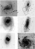 |
Fig. 1 Images of each galaxy studied and the WFPC2 field. First row, NGC 925 (Silberman et al. 1996), NGC 2541 (Ferrarese et al. 1998). Second row, NGC 3351 (Graham et al. 1997), NGC 3621 (Rawson et al. 1997). Third row, NGC 4548 (Graham et al. 1997), NGC 5457 (BKS 1996). |
Massive young stars have been considered to be born mostly inside stellar groupings and not in isolation, but there is an open debate about this in the recently published literature. A study of SMC (Maragoudaki et al. 2001; Livanou et al. 2006) showed that most of the newly born stars are within small structures. In the solar neighborhood, near infrared observations suggested that most of the stars are born in clusters (Lada & Lada 2003; Porras 2003). At least 20% of the young stars and possibly all of them are formed in clusters or associations in the Antennae galaxies (Fall 2004). More recently, Bressert et al. (2010) have studied the surface densities of young stellar objects (YSOs) in the solar neighborhood from surveys of the Spitzer Space Telescope. It was reported that the star formation process is hierarchical, that only a small fraction of the YSO was formed in dense environments, and finally that there is no evidence for discrete modes of star formation. A study of a number of galaxies with HST/ACS and HST/WFPC2 images by Silva-Villa & Larssen (2011) concludes that 2%–10% of the star formation is taking place in clusters compared to the global star formation rate. Gieles et al. (2012) agree with Bressert et al. (2010) that local surface density is not a useful tool for separating clusters from field stars, but suggest that the distribution of surface densities cannot be used to prove that not all stars are formed in dense environments.
Different authors use the name “stellar association” for different kinds of stellar groups (Ivanov 1996), with dimensions depending on the identification criteria, distance of the galaxy, and image scale (Hodge 1986). The first who proposed the name stellar association was Abartsumian (1949) and later Blaauw (1964) described associations as a large gravitationally unbound stellar group of O and B stars. The processes used so far to identify an OB association were based on the subjective selection criteria of each observer (Lucke & Hodge 1970; Hodge 1986). As a consequence it was difficult to compare results of various studies and even between observations of different areas made by the same observer. Battinelli (1991) proposed the distance between two stars as a criterion for a star to be considered as a member of an OB association. His method, the path linkage criterion, provided an objective tool to the identification process.
Efremov (1987) categorized star forming regions into associations, aggregates, complexes and supercomplexes based on their size (Maragoudaki et al. 1998; Livanou et al. 2007). In this paper the division of the previous studies is adopted, therefor the size of associations is considered to be from 30 pc to 100 pc. The distance among members of the group was also used as a criterion in our study implemented with the use of a friend-of-friend (FOF) algorithm which was invented by Huchra & Geller (1982) and is a cluster-finding technique. The algorithm searches for pairs of objects that they are closer than a cut-off distance limit. The original algorithm was used in finding groups and clusters of galaxies. Moreover, the distinction of groups into four categories led us, instead of using one value for the distance parameter or search radius (Ds), to select four values through the algorithm, one for each group category.
2. Observational data
The six galaxies we studied were part of the HST Extragalactic Distance Scale Key Project, an effort to study Cepheid variables in order to constrain the Hubble constant (Kennicutt et al. 1995). A picture of each galaxy is presented in Fig. 1 with the WFPC2 field superposed. Details about the studied galaxies can be found in Table 1. All images used for our purpose were taken with the Wide Field and Planetary Camera 2 (WFPC2), which featured four chips. Three in the Wide Field Camera (WFC), which was arranged in an L-shape, and the planetary camera (PC) with a higher resolution than the other three. The fields of view of each of the WFC chips covered 1′,33 × 1′, 33 and of the PC covered 35′′ × 35′′.
Details of observations.
Photometry.
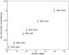 |
Fig. 2 Mv limit from 50% completeness in each galaxy. |
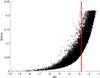 |
Fig. 3 Mv error in NGC 925. The vertical line indicates the 50% completeness Mv limit. |
Data were taken using HST/WFPC2 images and the filters F555W(V) and F814W (I) and were retrieved from the HST data archive1. The data were reduced using the HSTphot photometry package (Dolphin 2000). A PSF photometry was used and the median errors and other details of the photometry are given in Table 2. Several images of the same filter for each galaxy were combined using the coadd subroutine of the HSTphot to produce very deep exposures and increase the photometry magnitude limit. The list of stars for each galaxy was used to produce a fake image in order to perform the photometry again and to estimate the completeness. The faintest Mv limit for 50% completeness for our sample was Mv = −4 in NGC 4548 (the most distant of the galaxies). The Mv limit for each galaxy is shown in Fig. 2, and in Fig. 3 an indicative plot of the Mv and the photometry errors is presented for NGC 925.
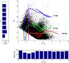 |
Fig. 4 CMD of NGC 925 (with isochrones for 10, 50, and 100 Myr, Marigo et al. 2008) and errorbar for V − I. |
NGC 925 is one of the galaxies studied in our paper and it is given below as an example of the process followed in selecting a sample of young main sequence bright stars for the algorithm. Hereafter whenever a bright star sample is mentioned, it refers to young main sequence stars. NGC 925 lies at a distance of 9.29 Mpc (Silbermann et al. 1996), is classified as an SBcII-III galaxy by Sandage & Tamman (1981) and as an SBS3 galaxy by de Vaucouleurs et al. (1991) with inclination of 55.8° (de Vaucouleurs et al. 1991). After the photometry for the field of view of WFPC2, a catalog of stars was produced with 25 584 members, and after imposing the cutoff limit the catalog was limited to 3930 members. The final number of bright main sequence stars selected for this investigation in each galaxy are listed in Table 2. The value of V − I < 0.23 was selected as in Bresolin et al. (1998) who studied the same galaxies. We tested different values of V − I, which were lower and higher than the one selected. The lower V − I value (0.2) reduces the population of the bright star catalog for all galaxies by 5% on average for the galaxy sample, compared to the number of stars reported in the paper. At the other end (V − I < 0.3), the catalog was increased by 10%, but the possibility that we may have selected later spectral types is increased. In Fig. 4 we can see the CMD plotted for NGC 925, the vertical line is the imposed V − I cutoff limit (V − I < 0.23), and the horizontal line is the 50% completeness limit. Tests with the Besancon model (Robin et al. 2003) were carried out for the catalog of each galaxy studied. The contamination of the catalog with stars on the line of sight was insignificant. The plotted Padova isochrones (Marigo et al. 2008) available at the time of the investigation provide an estimate of the range of ages for our star sample, between 10 and 100 Myr. Correction for extinction was applied for all colors following Allen & Shanks (2004).
NGC 2541 belongs to the NGC 2841 group (de Vaucouleurs 1978) near the border of Ursa Major and Lynx and is classified as Sc(s)III (Sandage & Tamman 1987), inclination 55° (Bottinelli et al. 1985b). The distance of the NGC 2541 was estimated to 12.4 Mpc (Ferrarese et al. 1998). At a distance 10.05 Mpc (Graham et al. 1997), NGC 3351 is a bright barred spiral galaxy with 40° inclination (Rubin et al. (1975). It was classified by Sandage & Tamman (1981) as SBb(r)II and is a member of the Leo I group of galaxies. NGC 3621 is a relatively isolated spiral, classified as Sc II.8 (Sandage & Tamman 1981), and it lies at a distance of 6.3 Mpc (Rawson et al. 1997). Gardiner & Whiteoak (1977) reported an inclination value of 51°. NGC 4548 belongs to the Virgo Cluster (de Vaucouleurs & de Vaucouleurs 1973; Bingelli et al. 1987), which is a well-resolved spiral with galaxy type SBb(rs)I-II (Sandage & Tamman 1981), and lies at a distance of 15.9 Mpc (Graham et al. 1999) with 37° inclination (Rubin et al. 1999). NGC 5457 or M101 is a luminous spiral with morphological type SAB(rs)cd (de Vaucouleurs et al. 1991), estimated distance 7.4 Mpc (Kelson et al. 1995), and 18° inclination (Bosma et al. 1981).
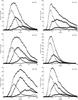 |
Fig. 5 Ds vs. the number of groups for each galaxy studied. Total number of groups (squares), associations (crosses), aggregates (triangles), complexes (circles), supercomplexes (dots). |
3. Automatic search for young stellar structures
3.1. Application of the friend of friend algorithm
Prior to the application of the FOF algorithm, two steps must be performed. The first one was to select young main sequence stars that was described in Sect. 2. The next and final step prior to applying the algorithm was to calculate distances between all stars, which was necessary since the distance value will determine if two stars are members of the same structure.
Ds values per size category for each galaxy studied.
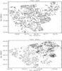 |
Fig. 6 All groups found for galaxies NGC 925 and NGC 2541. |
The range of the Ds (search radius) values that would be inserted in the algorithm was set from 1 to 200 pc with a step of 1 pc. Tests were performed for step values higher and lower than the value of 1 pc used throughout the paper. An increase in the width of the step may result in omitting several groups, depending on the increase. As the width of the step increases, the number of groups that we will lose increases as well. Another matter is that the value of max Ds will also change. By increasing the width there is also an increase in the error of the max Ds value estimation. By using a 0.1 pc step in the algorithm, the number of groups formed and the max Ds value did not vary significantly or did not vary at all. The computational time was increased significantly so the decision was made to choose a step value of 1 pc. The algorithm was applied to all galaxies’ star catalog for each Ds value, and when structures were detected, their size (the maximum distance between its members) was estimated in order to be categorized appropriately. In this all Ds values are associated with the number of structures found for every size category after applying the algorithm for that specific value. After completing the process for the whole Ds range, a plot for each galaxy was plotted (Fig. 5). This kind of graph was created by plotting pairs of Ds value and the number of groups found for that specific value for each category of group, essentially producing five plots, one for each size category and one for the total number of groups found as described in Sect. 2. The maximum point of each of the four colored plots was identified and the FOF algorithm was applied again, now using only the four Ds values specified by the above process (Table 3). The center of each group is calculated as the mean Right Ascension and Declination of their star members. Subsequently, the groups found are plotted in Figs. 6–8. For each galaxy a catalog of all identified groups has been produced. The complete catalogs are available at the CDS. In the printed version we present in Table 4 the first ten entries of NGC 925.
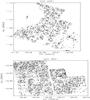 |
Fig. 7 All groups found for galaxies NGC 3351 and NGC 3621. |
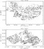 |
Fig. 8 All groups found for galaxies NGC 4548 and NGC 5457. |
Catalog of groups identified in NGC 925.
3.2. Description of our method
The automated method used in this paper is based on path linkage criterion (PLC) introduced by Battinelli (1991), an objective method to identify OB associations. The main intention of the method was to apply an objective criterion to the identification process. Two stars belong to the same group only if they are at a distance less or equal to a predefined value of Ds. In that principle we investigated the whole of our star catalogs. One important question needed to be addressed in this method is the value of search radius for which our star catalogs will be investigated in order to identify small (associations and aggregates) and larger structures (complexes and supercomplexes) in order to study the possible hierarchical structures. For each value of Ds that we set as a limit for two stars to be considered members of the same class, a number of groups (n) are found through the algorithm. Battinelli argued that the value of Ds that produces the maximum number of groups is the one that should be used. The applied FoF algorithm is a statistical approach, and our intention is to study all of the possible structures that can be identified in a certain field of study. If we use a lower Ds value than the one producing the maximum number of formations then we will end up losing a number of groups. As we move on to higher Ds values, groups start to merge, and that will again result in omitting a number of groups and in detecting larger structures as well, due to merging, than the ones that we would have detected if the maximum was selected. To determine that value, the algorithm is applied for a set of Ds values. For each step in the Ds values set, a list of pairs (Ds and n) is derived and plotted (Fig. 5, plot of the total number of stars).
Number of groups for each group type and their characteristics for each galaxy.
As the distance value increases and we move farther away from the maximum, some of the smaller formations are starting to merge, so that we detect fewer groups than we did before. If the plot exhibits a secondary maximum or a plateau, it is an indication of the existence of larger formations (Battinelli et al. 1996). With a further increase in Ds the larger groups merge and the number of groups decreases again. As a result we can use both maxima to find small formations (primary maximum point of the plot) and larger ones (secondary maximum). If the field of study is relatively small, then the plot may indicate the value of Ds in order to identify formations that are larger than associations (secondary maximum). On the other hand, if the field of study is large, as is the case for the galaxies studied here, the application of PLC produces a smooth plot, where the only point easily identified is the function’s maximum. Thus larger formations like complexes remain mostly undetected.
To detect larger structures, we could divide the large area into smaller subsections, hence apply the identification process into each subsection. The problem with that is that by dividing the area we may lose some larger formations that overlap two or more adjoining subsections or formations on the borderlines between the subsections. In addition by dividing the studied area the size of each subsection has to be considered, because it can impose an upper limit on the structures to be detected. Also, if we end up with a significant number of smaller areas, the process becomes more time-consuming and the number of large structures that we lose increases. Another possible approach was to select a specific area of the field that is small enough to produce the graph that is useful for the identification process. That approach is susceptible to the subjective selection of the researcher and lacks the information of hierarchy on large scales.
The field of each galaxy studied here produced a smooth plot of Ds vs. number of groups. That made the identification of larger scale structures almost impossible. Thus applying the FOF algorithm using the Ds value associated with the maximum number of groups would have given us mostly small stellar structures, associations, and aggregates according to the size distinction used here and in some galaxies a few complexes. Another issue to consider is that by using that particular Ds value, we detect the maximum number of small groups but not the maximum number of associations or any of the other size categories. To overcome both issues, it was decided to introduce another criterion into our algorithm, the size of the formations found. We divided the stellar structures into the four main types introduced by Efremov (1987), associations (from 30 to 100 pc in size), aggregates (from 100 to 300 pc), complexes (from 300 to 1000 pc), and supercomplexes (from 1000 pc and above), so the code produces four graphs, one for each category (Fig. 5). The algorithm was applied again for each one of the four indicated Ds values (the maximmun point of each of the four new plots), and all groups that were identified in each FOF application were cataloged and mapped. Using the approach described above, the algorithm can be used in identifying structures with varying size without any limit posed by the algorithm. We can combine our search for other types of structures, whether smaller or larger, in order to evaluate their spatial distribution even for large fields.
3.3. Properties of the four group types
An overview of the properties of the structures found per category for each galaxy studied is given in Table 5. The total number of groups per type, the average and median value of each group type’s size, and the mean number of group members are shown. As an example, the average values that we obtained per category for NGC 925, 356 associations with average size 67 pc and 4 members, 326 aggregates with average 174 pc in size and 8 members, 80 complexes with size 512 pc and 32 members, 13 supercomplexes with size 1527 pc and 195 members. Almost 60% of the associations have three members, and 95% contain up to five members. The number of groups of associations and aggregates constitute 88% of our total groups found in each galaxy and their size distribution is given in Fig. 9 (all groups with size no more than 300 pc).
Density is given as the number of stars per square parsec. As we can see from the plot in Fig. 10, the associations present higher values of surface density than all the other types of groups. In Fig. 11 the distribution of densities in each galaxy is given. It is noteworthy that the histograms are similar for the galaxies of our sample.
4. Discussion
The method used in this study can identify at the same time a number of different types of stellar structures that vary in size. The FOF algorithm runs through a range of distance (search radius) values to find the one presenting the maximum population number of each particular group type that we want to be identified instead of searching for the maximum number of all groups and then searching among that sample for a specific type of group.
Comparing the two methods in the case of associations, the maximum point if we applied PLC (which is represented by the plot of the total number of groups) without the added size criterion, presented a reduced number of associations and an increased number of aggregates compared to the number detected using the specific plot for that size category. It should be noted that the other group types, complexes, and supercomplexes were limited to a very small number for PLC, or they were not detected at all thus requiring further analysis.
Using NGC 925 in Fig. 5 as an example, the maximum point of the total groups plot is at Ds = 59 pc and n = 328 groups in total and, in particular, 197 associations, 118 aggregates and 12 complexes. Using the associations plot maximum point, Ds = 45 pc, we detected 239 associations. In each algorithm application at the Ds values indicated by the maximum point of the plots of the other size categories, we detected associations again and by removing duplicate entries (the same associations detected in more than one FOF application), the total number of associations in our catalog is 356. Similarly we applied our process for each size category, detecting more structures than by applying FOF once.
Setting a size limit for each group type can affect the Ds value determination by the algorithm. The Ds value is actually the distance radius at which the algorithm searches around each star of the catalog, in order to find whether any other star lies in that area. If that is the case, both will be considered members of the same group. When the algorithm moves to the next star follows the same process and adds to the group any other star that lies within a distance defined by the Ds value. It is almost impossible to detect large structures using low Ds values. At some point there will be no stars within that distance to continue adding members into the group unless the local star density is very high. Even if the algorithm runs through a dense area, it is unlikely that Ds values around the associations’ maximum will detect structures larger than aggregates. As a result the large-scale structures are found with higher Ds values than small structures (associations). For the galaxies in our sample the Ds range for identifying associations was 39–59 pc. For aggregates the Ds value range was 58–97 pc, and for complexes and supercomplexes it was 73–179 pc and 96–200 pc, respectively. Even though there is an overlap in the Ds value range for each type of structure (usually caused by one of the six galaxies, otherwise the ranges would have been tighter), we can expect that for a structure with a specific size limit, the Ds value that would be used for the identification would be in a specific range. In that sense the type of structure that we are looking for “indicates” a loose range of Ds values and affects the resulting average sizes since its size limits are already defined. The selection of that Ds value is not arbitrary since the algorithm seeks the maximum point in each plot.
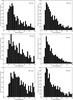 |
Fig. 9 Size distribution of associations and aggregates (groups with size up to 300 pc) for each galaxy studied. |
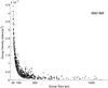 |
Fig. 10 Surface density of groups for varying group size. associations (30–100 pc), aggregates (100–300 pc), complexes (300–1000 pc), supercomplexes (>1000 pc). |
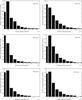 |
Fig. 11 Density distribution for each galaxy studied. |
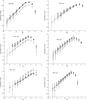 |
Fig. 12 Luminosity function for each galaxy studied: associations (crosses), aggregates (triangles), complexes (circles), supercomplexes (squares). |
4.1. Luminosity function
A luminosity function (LF) for every group category was produced for each galaxy in our study (Fig. 12). A best fit was obtained, and its slope was calculated. Even though the completeness of the data indicated a recovery of about 50% at V = 27 mag, the LF presented a breaking point around V = 26 mag, constraining the LF faint magnitude limit to Mv < − 4.5 or –4.0 mag, depending on the galaxy. The slope for associations presents similar values to those found by Bresolin et al. (1998, hereafter B98) for the same galaxies, with an average value of 0.59 (0.61 reported by B98). We would expect the LF for the other group types, especially for the larger sizes, complexes, and supercomplexes, to present steeper slopes than associations due to the larger number of faint members. Indeed, in all galaxies complexes and supercomplexes have larger slope values but the difference is small. This is due to the Mv limit in our LF, and the detection limit of the observations as the faintest stars within our selection criteria are up to –2.5 mag (the lower Mv limit for the galaxy sample varied from –2.5 to –4.0 mag). Since most of the small structures (associations and aggregates) are within the larger structures (complexes and supercomplexes) and the stellar content of the structures are not independent, the luminosity functions were not normalized.
4.2. Comparison with previous investigations
We compared our results with those derived in a number of studies of other galaxies, M101 and LMC (B98, Kennicut, Stetson 1996, BKS), LMC (Gouliermis et al. 2003), M33, M31, SMC (Battinelli et al. 1996), NGC 6822 (Karampelas et al. 2009; Gouliermis et al. 2010), and HST galaxies (Bresolin et al. 1998).
B98 studied the same sample of HST galaxies, using an FOF algorithm based on the PLC method of Battinelli. They selected various values for the minimum number of stars for each group (Nmin) and a search radius for each galaxy. They found a scale length for the associations around 80 pc, using the median values of group size found for each galaxy, for identified groups with sizes up to 200 pc. The difference with our reported size of associations can be explained by the criteria used in both studies in order to approach the term associations. Groups with upper size limit 200 pc contributed to the increased average value. If in our study the same criterion was applied, the average value for associations per galaxy would be close to the one found by B98 despite the differences in the average and median size values reported above. The size distribution for both studies peaked in the same range, 40–80 pc for B98 and 50–80 pc for this study. The scale length of ~80 pc was reported as well by BKS when comparing groups found in six galaxies, M101(NGC 5457), M31, M33, NGC 6822, LMC, and SMC, where the median value varied from 60 to 100 pc for a varying value of Nmin from 3 to 10. The size distribution of all galaxies presented a peak at the 40–80 pc except for M 31, were it was ~110 pc. Another contributing factor for the difference in reported sizes is the varying Nmin values. The increase in Nmin leads to identifying larger groups than when using lower Nmin values. Gouliermis et al. (2003) report an average size of associations of 86 pc for LMC, and a peak in the size distribution at 70 pc, and a number of studies for different galaxies was also presented as well where the average size of the associations varied from 65–93 pc. For NGC 6822 Gouliermis (2010) gives a lower average of 68 pc.
It should be noted that in the studies mentioned above, different criteria were used for what is considered an association, and the techniques used for the identification of stellar structures were not the same. The reported size distributions, though, peaked in the same range, 40–80 pc. The reported average sizes varied from 60 pc to 100 pc. Stellar formation structures that are larger than associations were also detected by our algorithm. Aggregates with average values varying, from 162–175 pc for size and 5–9 stars per group. Complexes with an average size from 500 to 517 pc and average number of members from 15–48. The final category, supercomplexes, was detected to have an average size from 1200–1600 pc and 74–311 members, where five of the six were in the range of 75–200. The average size for each group category seems to agree with previously reported typical sizes of structures larger than associations. For M31 van den Bergh (1964) identified groups of blue stars with average size ~500 pc. Efremov et al. (1987) identified star complexes ~600 pc average size. Magnier et al. (1993) found a large number of groups with sizes from 50–150, roughly the average values of associations and aggregates in our study, and a few larger structures ~400 pc in size. For the same galaxy, Battinelli et al. (1996) found hierarchical structures on two levels, the first with size ~100 pc and the second with a distribution of sizes from ~100 to ~800 pc with maximum at ~200 pc, in the middle of our aggregates range, and an indication of a peak at ~400 pc (complexes). Similar were the findings for LMC (Livanou et al. 2007) and NGC 6822 (Karampelas et al. 2009), where star complexes were detected in two ranges, from 150–400 pc, so roughly what we considered as aggregates. The second was 400–800 pc, in the complexes range.
It seems that surface density is correlated to the group size. The density of the structures seems to increase as the size decreases; most of the associations are denser than any other group except a small part of aggregates with sizes around the lower limit, 100 pc. Complexes and supercomplexes have the lowest surface density values. In Fig. 11, the surface density versus group size is shown for each of the studied galaxies, which is indicative of what was described above.
Hierarchical structure (Elmegreen & Efremov 1996; Maragoudaki et al. 2001; Livanou et al. 2006; Karampelas et al. 2009) is indicated in all six galaxies. Most of the associations and aggregates,which are small in size (about 65 pc and 160 pc respectively) and dense, are found to be lying inside the lagrer in size groups, complexes, and supercomplexes (about 500 pc and 1400 pc respectively), which also present the lower density values of all groups, as we can see in Figs. 6–8. In Fig. 7, the mapped structures of NGC 3351 cleary trace the spiral arm extended away from the nucleus and the central bar, where there are no structures, from north to south (top of the figure to the bottom). Similarly in NGC 4548 (Fig. 8), the identified structures trace the spiral arm from east to west (left to right in our figure) along the nucleus, located at the top of the figure.
It is common to find supercomplexes lying inside other supercomplexes as in NGC 3621 (Fig. 7), almost at the center of the figure where three supercomplexes are found, one inside the other. The smallest one was identified when we applied the FOF algorithm for Ds = 58 pc. The structure enclosing that supercomplex was found when the search radius increased at 73 pc, and the third, which is even larger was found using a search radius of 96 pc. Since the Ds value increases, the structures found are larger in size, and that is even more evident in large groups and mainly in supercomplexes.
5. Conclusions
In this paper a FOF algorithm was used to identify star forming structures in six HST galaxies. The algorithm was written based on Battinelli’s principles for the identifications of OB associations. We introduced a new criterion in the process, the group size. Groups were divided into specific size ranges as was suggested in the literature (associations, aggregates, complexes, and supercomplexes). Our algorithm now searches for one or more than one group type at the same time, indicating the appropriate Ds value, where the maximum number of groups were identified for each group type. It is capable of detecting small or larger structures, even in a large field of study. The detected groups were found within the size range reported in the literature. The associations were found to have an average size of ~65 pc and an average of around 4 members per group, the aggregates had an average in size ~165 pc and about eight stars per group, complexes were found to have an average size of ~500 pc and ~22 members and finally supercomplexes were found to be around ~1400 pc in size and to have ~150 stars. The detected groups provided strong indications of a hierarchical structure.
Acknowledgments
The authors would like to thank the anonymous referee for his constructive comments that have improved the final version of the publication. Also the authors would like to thank PRODEX/ESA for financial support, the National and Kapodistrian University of Athens (NKUA), and the National Observatory of Athens (NOA). All of the data presented in this paper were obtained from the Mikulski Archive for Space Telescopes (MAST). STScI is operated by the Association of Universities for Research in Astronomy, Inc., under NASA contract NAS5-26555. Support for MAST for non-HST data is provided by the NASA Office of Space Science via grant NNX09AF08G and by other grants and contracts.
References
- Allen, P. D., & Shanks, T. 2004, MNRAS, 347, 1011 [NASA ADS] [CrossRef] [Google Scholar]
- Ambartsumian, V. A. 1949, AZh, 26, 3 [Google Scholar]
- Battinelli, P. 1991, A&A, 244, 69 [NASA ADS] [Google Scholar]
- Battinelli, P., Efremov, Yu., & Magnier, E. A. 1996, A&A, 314, 51 [NASA ADS] [Google Scholar]
- Bosma, A., Goss, W. M., & Allen, R. J. 1981, A&A, 93, 106 [NASA ADS] [Google Scholar]
- Bottinelli, L., Gouguenheim, L., & Paturel, G. 1985, A&A, 59, 43B [Google Scholar]
- Binggeli, B., Tammann, G. A., & Sandage, A. 1987, AJ, 94, 251 [NASA ADS] [CrossRef] [Google Scholar]
- Blaauw, A. 1964, ARA&A, 2, 213 [NASA ADS] [CrossRef] [Google Scholar]
- Bresolin, F., Kennicut, R. C., Jr., & Stetson, P. B. 1996, AJ, 112, 1009 (BKS) [NASA ADS] [CrossRef] [Google Scholar]
- Bresolin, F., Kennicut, R. C., Jr., Ferrarese, L., et al. 1998, AJ, 116, 119 [NASA ADS] [CrossRef] [Google Scholar]
- Bressert, E., Bastian, N., Gutermuth, R., et al. 2010, MNRAS, 409, L54 [NASA ADS] [Google Scholar]
- de Vaucouleurs, G. 1978, ApJ, 224, 14 [NASA ADS] [CrossRef] [Google Scholar]
- de Vaucouleurs, G., & de Vaucouleurs, A. 1973, A&A, 28, 109 [NASA ADS] [Google Scholar]
- de Vaucouleurs, G., de Vaucouleurs, A., Corwin, H. G., et al. 1991, Third Reference Catalogue of Bright Galaxies (New York: Springer) [Google Scholar]
- Dolphin, A. 2000, PASP 112, 138 [Google Scholar]
- Efremov, Yu. N., & Chernin, A. D. 1994, Vistas Astron., 38, 165 [NASA ADS] [CrossRef] [Google Scholar]
- Efremov, Yu. N., & Elmegreen, B. G. 1998, MNRAS, 299, 588 [NASA ADS] [CrossRef] [MathSciNet] [Google Scholar]
- Efremov, Yu. N., Ivanov, G. R., & Nikolov, N. S. 1987, Ap&SS, 135, 119 [NASA ADS] [CrossRef] [Google Scholar]
- Elmegreen, B. G., & Efremov, Y. N. 1996, ApJ, 466, 802 [NASA ADS] [CrossRef] [Google Scholar]
- Fall, S. M. 2004, in The Formation and Evolution of Massive Young Star Clusters, eds. H. J. G. L. M. Lamers, L. J. Smith, & A. Nota, ASP Conf. Ser., 322, 399 [Google Scholar]
- Ferrarese, L., Bresolin, F., Kennicutt, R. C. Jr., et al. 1998, AJ, 507, 655 [Google Scholar]
- Gardiner, L. T., & Whiteoak, J. B. 1977, Australian J. Phys., 30, 187 [NASA ADS] [CrossRef] [Google Scholar]
- Gieles, M., Moeckel, N., & Clarke, C. J. 2012, MNRAS, 426, L11 [NASA ADS] [CrossRef] [Google Scholar]
- Gouliermis, D., Kontizas, M., Kontizas, E., et al. 2003, A&A, 405, 111 [NASA ADS] [CrossRef] [EDP Sciences] [Google Scholar]
- Gouliermis, D., Schmeja, S., Klessen, R. S., et al. 2010, A&A, 725, 1717 [Google Scholar]
- Graham, J. A., Phelps, R. L., Freedman, W. L., et al. 1997, AJ, 477, 535 [Google Scholar]
- Graham, J. A., Ferrarese, L., Freedman, W. L., et al. 1999, AJ, 516, 626 [Google Scholar]
- Hodge, P. 1986, IAUS, 116, 369 [Google Scholar]
- Huchra, J. P., & Geller, M. J. 1982, AJ, 257, 423 [Google Scholar]
- Ivanov, G. R. 1987, Ap&SS, 136, 113 [NASA ADS] [CrossRef] [Google Scholar]
- Karampelas, A., Dapergolas, A., Kontizas, E., et al. 2009, A&A, 497, 703 [NASA ADS] [CrossRef] [EDP Sciences] [Google Scholar]
- Kelson, D. D., Illingworth, G. D., Freedman, W. F., et al. 1996, AJ, 463, 26 [Google Scholar]
- Kennicutt, R. C. Jr., Freedman, W. L., & Mould, J. R. 1995, AJ, 110, 1476 [NASA ADS] [CrossRef] [Google Scholar]
- Lada, C. J., & Lada, E. A. 2003, ARA&A, 41, 57 [NASA ADS] [CrossRef] [Google Scholar]
- Livanou, E., Kontizas, M., Gonidakis, I., et al. 2006, A&A, 451, 431 [NASA ADS] [CrossRef] [EDP Sciences] [Google Scholar]
- Livanou, E., Gonidakis, I., Kontizas, E., et al. 2007, AJ, 133, 2179 [NASA ADS] [CrossRef] [Google Scholar]
- Lucke, P. B., & Hodge, P. W. 1970, AJ, 75, 171 [NASA ADS] [CrossRef] [Google Scholar]
- Magnier, E. A., Battinelli, P., Lewin, W. H. G., et al. 1993, A&A, 278, 36 [NASA ADS] [Google Scholar]
- Maragoudaki, F., Kontizas, M., Kontizas, E., et al. 1998, A&A, 338, L29 [NASA ADS] [Google Scholar]
- Maragoudaki, F., Kontizas, M., Morgan, D. H., et al. 2001, A&A, 379, 864 [NASA ADS] [CrossRef] [EDP Sciences] [Google Scholar]
- Marigo, P., Girardi, L., Bressan, A., et al. 2008, A&A, 482, 883 [NASA ADS] [CrossRef] [EDP Sciences] [Google Scholar]
- Porras, A., Christopher, M., Allen, L., et al. 2003, AJ, 126, 1916 [NASA ADS] [CrossRef] [Google Scholar]
- Robin, A. C., Reyle, C., Derriere, S., et al. 2003, A&A, 409, 523 [NASA ADS] [CrossRef] [EDP Sciences] [Google Scholar]
- Rubin, V. C., Ford, W. K., & Peterson, C. J. 1975, ApJ, 199, 39 [NASA ADS] [CrossRef] [Google Scholar]
- Rubin, V. C., Waterman, A. H., & Kenney, J. P. D. 1999, AJ, 118, 236 [NASA ADS] [CrossRef] [Google Scholar]
- Sandage, A., & Bedke, J. 1988, Atlas of Galaxies Useful for Measuring the Cosmological Distcane Scale (Washington, DC: NASA) [Google Scholar]
- Sandage, A., & Tamman, G. A. 1981, A Revised Shapley-Ames Catalog of Bright Galaxies (Washington, DC: Carnegie Inst. Washington) [Google Scholar]
- Sandage, A., & Tamman, G. A. 1987, A Revised Shapley-Ames Catalog of Bright Galaxies (Washington, DC: Carnegie Inst. Washington) [Google Scholar]
- Rawson, D. M., Macri, L. M., Mould, J. R., et al. 1997, AJ, 490, 517 [Google Scholar]
- Silbermann, N. A., Harding, P., Madore, B. F., et al. 1996, AJ, 470, 1 [Google Scholar]
- Silva-Villa, E., & Larsen, S. S. 2011, A&A, 529, 59 [Google Scholar]
- Tully, R. B. 1980, ApJ, 237, 390 [NASA ADS] [CrossRef] [Google Scholar]
- van den Bergh, S. 1964, ApJS, 9, 65 [NASA ADS] [CrossRef] [Google Scholar]
All Tables
All Figures
|
Fig. 1 Images of each galaxy studied and the WFPC2 field. First row, NGC 925 (Silberman et al. 1996), NGC 2541 (Ferrarese et al. 1998). Second row, NGC 3351 (Graham et al. 1997), NGC 3621 (Rawson et al. 1997). Third row, NGC 4548 (Graham et al. 1997), NGC 5457 (BKS 1996). |
| In the text | |
|
Fig. 2 Mv limit from 50% completeness in each galaxy. |
| In the text | |
|
Fig. 3 Mv error in NGC 925. The vertical line indicates the 50% completeness Mv limit. |
| In the text | |
|
Fig. 4 CMD of NGC 925 (with isochrones for 10, 50, and 100 Myr, Marigo et al. 2008) and errorbar for V − I. |
| In the text | |
|
Fig. 5 Ds vs. the number of groups for each galaxy studied. Total number of groups (squares), associations (crosses), aggregates (triangles), complexes (circles), supercomplexes (dots). |
| In the text | |
|
Fig. 6 All groups found for galaxies NGC 925 and NGC 2541. |
| In the text | |
|
Fig. 7 All groups found for galaxies NGC 3351 and NGC 3621. |
| In the text | |
|
Fig. 8 All groups found for galaxies NGC 4548 and NGC 5457. |
| In the text | |
|
Fig. 9 Size distribution of associations and aggregates (groups with size up to 300 pc) for each galaxy studied. |
| In the text | |
|
Fig. 10 Surface density of groups for varying group size. associations (30–100 pc), aggregates (100–300 pc), complexes (300–1000 pc), supercomplexes (>1000 pc). |
| In the text | |
|
Fig. 11 Density distribution for each galaxy studied. |
| In the text | |
|
Fig. 12 Luminosity function for each galaxy studied: associations (crosses), aggregates (triangles), complexes (circles), supercomplexes (squares). |
| In the text | |
Current usage metrics show cumulative count of Article Views (full-text article views including HTML views, PDF and ePub downloads, according to the available data) and Abstracts Views on Vision4Press platform.
Data correspond to usage on the plateform after 2015. The current usage metrics is available 48-96 hours after online publication and is updated daily on week days.
Initial download of the metrics may take a while.