| Issue |
A&A
Volume 552, April 2013
|
|
|---|---|---|
| Article Number | A110 | |
| Number of page(s) | 9 | |
| Section | Galactic structure, stellar clusters and populations | |
| DOI | https://doi.org/10.1051/0004-6361/201220842 | |
| Published online | 10 April 2013 | |
Reddening and metallicity maps of the Milky Way bulge from VVV and 2MASS⋆
III. The first global photometric metallicity map of the Galactic bulge
1
European Southern Observatory,
Casilla 19001,
Santiago 19,
Chile
e-mail:
ogonzale@eso.org
2
European Southern Observatory, Karl-Schwarzschild-Strasse 2, 85748
Garching,
Germany
e-mail: mrejkuba@eso.org; evalenti@eso.org
3
Departamento Astronomía y Astrofísica, Pontificia Universidad
Católica de Chile, Av. Vicuña
Mackenna 4860, Stgo., Chile
e-mail: mzoccali@astro.puc.cl; dante@astro.puc.cl
4
The Milky Way Milennium Nucleus, Av. Vicuña Mackenna 4860, 782-0436
Macul,
Santiago,
Chile
5
Vatican Observatory, V 00120
Vatican City State,
Italy
6
Departamento de Ciencia Fisicas, Universidad Andres
Bello, Santiago,
Chile
Received: 3 December 2012
Accepted: 30 January 2013
Aims. We investigate the large-scale metallicity distribution in the Galactic bulge using large spatial coverage to constrain the bulge formation scenario.
Methods. We use the VISTA variables in the Via Lactea (VVV) survey data and 2MASS photometry, which cover 320 sqdeg of the Galactic bulge, to derive photometric metallicities by interpolating the (J − Ks)0 colors of individual red giant branch stars based on a set of globular cluster ridge lines. We then use this information to construct the first global metallicity map of the bulge with a resolution of 30′ × 45′.
Results. The metallicity map of the bulge revealed a clear vertical metallicity gradient of ~0.04 dex/deg (~0.28 dex/kpc), with metal-rich stars ([Fe/H] ~ 0) dominating the inner bulge in regions closer to the Galactic plane (|b| < 5). At larger scale heights, the mean metallicity of the bulge population becomes significantly more metal poor.
Conclusions. This fits in the scenario of a boxy bulge originating from the vertical instability of the Galactic bar, formed early via secular evolution of a two-component stellar disk. Older metal-poor stars dominate at higher scale heights due to the non-mixed orbits of originally hotter thick disk stars.
Key words: Galaxy: bulge / Galaxy: abundances / Galaxy: formation / stars: abundances
© ESO, 2013
1. Introduction
In the hierarchical scenario of galaxy formation, the early mass assembly of galaxies is dominated by merger processes that favor the formation of spheroids (Toomre 1977). This violent and relatively fast process produces the present day elliptical galaxies. However, when the spheroids are accompanied by the (re-)growth of stellar disk (Kauffmann et al. 1999; Springel & Hernquist 2005), they receive the name of classical bulges.
Classical bulges are expected to share the same observational properties of elliptical galaxies. Their light profiles are well fitted by a Vaucouleurs-like profile with n ~ 4 (e.g., Gadotti 2009), and their stars show hot dynamics dominated by velocity dispersion (e.g., Gadotti 2012). An important point is that the rotation of classical bulges is observed to be non-cylindrical, therefore showing a decrease in rotation velocity at increasing height from the plane (e.g., Emsellem et al. 2004). Since classical bulges are formed violently in fast and early processes of collisions and mergers, stars in classical bulges are expected to have formed mostly from the starburst in the early times, with little or no star formation since then. For this reason, classical bulges are expected to be composed predominantly of old stars (~10 Gyr) (e.g., Renzini 1998). They have enhanced abundance ratios (Peletier et al. 1999; Moorthy & Holtzman 2006; MacArthur et al. 2008) and often show metallicity gradients, going from metal-poor stars in the outskirts to a more metal-rich population towards the center. (see, for example, Jablonka et al. 2007).
Given that the classical bulge formation scenario is connected to the rate of merger events, this is expected to be the dominant process in the early evolution of galaxies (Kormendy & Kennicutt 2004). Later on, secular evolution processes become important, re-arranging stellar material from a settled galactic disk. Disks instabilities, such as the presence of spiral arms, are expected to induce the formation of bars in the inner regions of a galactic disk (Combes & Sanders 1981; Weinberg 1985; Debattista & Sellwood 1998; Athanassoula & Misiriotis 2002). Indeed, galactic bars are a very common phenomena, found in ~60% of spiral galaxies in the local universe (e.g., Eskridge et al. 2000).
Although disks are thin galactic components, bars might become thicker because of the vertical resonances and buckle of the plane of the galaxy. For this reason, galaxies, when observed edge-on, often show a central component that swells out of the disk with a boxy, peanut, or even X-shape (e.g. Bureau et al. 2006; Patsis et al. 2002). These structures have been seen in numerous simulations as the result of the development of vertical instabilities from the initially thin stellar bar (Athanassoula 2005; Debattista & Williams 2004; Debattista et al. 2006; Martinez-Valpuesta et al. 2006).
The dynamical and structural properties of boxy bulges are well constrained from models and observations. However, the properties of their stellar populations are less clear than in the case of classical bulges. In fact, a variety of stellar populations are observed within bars (e.g., Gadotti & de Souza 2006; Pérez et al. 2009). In practice, since boxy bulges are bars thickened by vertical instabilities, the null hypothesis would be that they should hold similar ages as their parent disks. A similar case would be expected for the metallicity and alpha elements abundances. However, Freeman (2008) suggested that age and abundance gradients could be present in boxy bulges. Older, more metal-poor stars would have more time to be scattered to larger distances from the plane by the buckling process, thereby establishing a negative metallicity and positive age gradient. The presence and strength of such gradients would then depend on the chemical enrichment history of the parent disk material and the timescale of the buckling instability to form the boxy bulge.
The brightness profiles of boxy bulges are less centrally concentrated than those of classical bulges and are better fitted by light profiles with a lower sersic index (e.g., Kormendy & Bruzual A. 1978; Gadotti 2009). What is probably the most characteristic property of boxy bulges is that they present cylindrical rotation patterns. This means that the rotation velocity within a boxy bulge does not change with height above the galactic plane (e.g., Kormendy & Illingworth 1982; Combes et al. 1990; Athanassoula & Misiriotis 2002; Shen et al. 2010).
The presence of a central bar has important consequences for the subsequent evolution of the galaxy, redistributing the angular momentum and matter in the disk. In particular, it causes the loss of angular momentum of the molecular gas settled in the rotating disk, inducing its infall process into the inner regions of the galaxy. The gas, slowly fueling into the center, produces a slow star-formation process that results in the formation of a disk-like component in these inner regions. We refer to these structures as pseudo-bulges. The brightness of pseudo-bulges can be fitted with a very disk-like, exponential light profile, and the bulges are observed as flat, rotation-supported structures. Also, because gas fuels very slowly into the center due to the presence of the bar, the star formation is expected to be slow and continuous. A direct consequence is that pseudo-bulges host young stellar populations and are dominated by metal-rich stars with solar alpha element abundances.
As described before, boxy bulges are thickened bars; these bars are, in fact, disk phenomena resulting from internal processes of secular evolution. The absence of an external factor in the formation process of boxy bulges and the fact that both bars and boxy bulges are formed out of originally disk material, as opposite to the classical bulge scenario, led different authors to refer to them as pseudo-bulges. This is also qualitatively supported by the pseudo-bulge definition in the review of Kormendy & Kennicutt (2004), where they say: “..if the component in question is very E-like, we call it bulge; if it is more disk-like, we call it a pseudo-bulge”. The morphology of thickened bars is certainly not E-like (Bureau et al. 2006). However, to avoid confusion during our analysis, we refer to them as boxy bulges and not pseudo-bulges.
The above scenarios for bulge formation and their properties, which are mostly based on the study of bulges in nearby galaxies, have been recently challenged by the observation of galaxies at redshift ~2, i.e., at a lookback time comparable to the ages seen in classical bulges. At this redshift, disk galaxies are observed to hold large, rotating disks with a very high gas fraction and velocity dispersion, which is significantly different from local spirals (Genzel et al. 2006, 2008; Förster Schreiber et al. 2009; Tacconi et al. 2010; Daddi et al. 2010). Massive gas clumps form in these gas-rich galaxies via disk instabilities; They then interact and likely merge in the center of the disk. This violent process naturally leads to the rapid formation of a bulge over timescales of a few 108 yr, much shorter than that typically ascribed to secular instabilities in local disk galaxies (Immeli et al. 2004; Carollo et al. 2007; Elmegreen et al. 2008), thereby resulting in old, α-element enhanced, present day stellar populations (Renzini 2009; Peng et al. 2010) of both bulge and disk formed at the early cosmic epoch.
With the exception of the Milky Way and M 31 (Jablonka & Sarajedini 2005), the observational studies of the central components of galaxies are strongly challenged by the impossibility of resolving individual stars due to crowding and blending in high stellar density regions of distant galaxies. In this context, the Milky Way bulge, one of the major components of the Galaxy, can be studied at a unique level of detail thanks to its resolved stellar populations, which hold the imprints of how our Galaxy formed and evolved. Thus, a better understanding of the Milky Way bulge will provide solid constraints to interpret observations of extragalactic bulges and for a detailed comparisson with galaxy formation models.
The place of the Milky Way within these different bulge formation scenarios is far from being understood. The Galactic bulge structure is observed to be dominated by a stellar bar (Stanek et al. 1997) oriented ~25 deg with respect to the Sun-Galactic center line of sight (Stanek et al. 1997; López-Corredoira et al. 2005; Rattenbury et al. 2007; Gonzalez et al. 2012; Nataf et al. 2012). While the observed age of the bulge stars is 10 Gyr or older, based on deep photometric studies in a few low extinction windows (Zoccali et al. 2003; Clarkson et al. 2011), Bensby et al. (2012) found a non-negligible fraction of younger stars based on a microlensing study. A vertical metallicity gradient has been observed along the bulge minor axis (Zoccali et al. 2008; Johnson et al. 2011) that most likely flattens in the inner regions (Rich et al. 2007). In addition to the population of stars associated with a metal-rich, alpha-poor stellar bar, there are indications of a distinct component dominated by more metal-poor, alpha-enriched stars showing hot kinematics that resemble those of a classical bulge (Babusiaux et al. 2010; Hill et al. 2011; Gonzalez et al. 2011a; Uttenthaler et al. 2012). Furthermore, significant evidence is now available suggesting that the Galactic bulge is X-shaped in the outer regions (McWilliam & Zoccali 2010; Saito et al. 2011), as expected from the buckling instability processes of the bar. However, the metal-poor stars do not seem to follow the same spatial distribution (Ness et al. 2012).
Such complex sets of properties for the Galactic bulge are the result of the detailed study of discrete fields, mostly concentrated along the minor axis, especially in the case of chemical abundances. A larger, more general mapping of these properties is the necessary bridge between the detailed studies of the Galactic bulge and those of external bulges, where integrated light studies can only provide us with general information.
In Gonzalez et al. (2011b, Paper I), we have shown a procedure to build multiband near-infrared (near-IR) catalogs using the VISTA Variables in the Via Lactea (VVV) public survey data. We then used these to derive a complete, high-resolution extinction map of the Galactic bulge, based on the color information of red clump (RC) giant stars. The extinction map was presented in Gonzalez et al. (2012, Paper II), together with a discussion of the important implications of its use in bulge studies. One of the improvements is the availability of a de-reddened RC feature in the luminosity function that allows us to trace the mean distance of stars towards different regions of the bulge, the so-called RC method. The mean distance to each line of sight allows us then to place our photometric catalogs on the absolute plane and derive photometric metallicity distributions. In Paper I we tested the method by comparing these photometric metallicity distributions for regions along the bulge minor axis, where accurate spectroscopic metallicities are available. We found a remarkable agreement between both methods. In this article, the last of the series, we extend the derivation of photometric metallicities to the rest of the region covered by the VVV survey. We provide for the first time the global view of the metal content of bulge stars and their gradients as if we were looking at the Milky Way as an external galaxy.
2. The data
We use the public VVV first data release (DR1) catalog Saito et al. (2012). For a complete description of the survey and the observation strategy we refer the reader to Minniti et al. (2010). A detailed description of the combination of the tile-based source lists and their calibration is given in Paper I. Methods used in Paper I and Paper II are based on the analysis of the RC properties, which are restricted to a magnitude range well covered by the VVV survey photometry: across ~320 sqdeg of the Galactic bulge and spanning from −10 < l < 10 and −10 < b < +5. For this final part of the project, we require upper red giant branch (RGB) photometry to derive photometric metallicities by color interpolation between globular cluster ridge lines. As described in other articles (Gonzalez et al. 2011b; Saito et al. 2012), VVV photometry suffers from saturation for stars brighter than Ks = 12, which corresponds to the upper RGB region in the bulge color-magnitude diagrams (CMD) required for the color interpolation. For this reason, in Paper I, we constructed VVV multiband catalogs and calibrated them into the 2MASS system, so that we could later replace the saturated range of magnitudes with those of 2MASS photometry.
The VVV-2MASS calibration procedure is based on the comparison of stars flagged in 2MASS with high photometric quality in all three bands in the magnitude range between 12 < Ks < 13. This magnitude range avoids the saturated stars in VVV, while being bright enough to ensure a sufficient number of 2MASS sources with accurate photometry for the calibration. The zero point was calculated and applied individually to each VVV tile catalog. Finally, stars with Ks < 12 mag were removed from the VVV catalog and replaced with 2MASS sources.
Since 2MASS is severly affected by crowding in the regions close to the Galactic plane, we restrict our analysis for latitudes |b| > 2. This restriction also helps to avoid the high extinction regions where some differential reddening, in variation scales smaller than 2′ (the resolution of the bulge extinction map from Paper II), could be present.
3. Extinction and mean distances
By applying the extinction correction derived for the whole bulge on a spatial resolution of 2′ (|b| < 4), 4′ (4 < |b| < 6), or 6′ (b > 6′) (Paper II) and using the extinction law of Cardelli et al. (1989), the de-reddened luminosity function is derived for each line of sight in the bulge. The distances to these lines of sight are then derived by applying the equation  (1)We adopted MKs = −1.55 for the RC luminosity of a 10 Gyr old population with solar metallicity (Salaris & Girardi 2002; Pietrinferni et al. 2004; van Helshoecht & Groenewegen 2007), which is an average value appropriate for the bulk of the Milky Way bulge stars (Zoccali et al. 2003). However, the intrinsic magnitude of the RC (MKs) is known to have a certain dependence on metallicity. Although this dependence is neglected by most studies, a large metallicity gradient present in the bulge could bias our own metallicity calculation if a single MKs value is adopted for the whole bulge. In order to take into the account the (expected) presence of the metallicity variations, we apply the metallicity correction term (ΔMKs). As a consequence, we adopt an iterative process, which is described described in the next section, to derive the fully consistent distance and metallicity for each line of sight.
4. Photometric metallicities
The method to derive photometric metallicities in this work is based on the interpolation of the dereddened (J − Ks)0 colors of upper RGB stars between ridge lines of globular clusters with well-know metallicities derived from spectroscopy. In Paper I we compared the photometric metallicity distribution along the bulge minor axis to that of high-resolution spectroscopy for the same regions. We observed a very good agreement between both results; in particular, the photometric results reproduced the minor axis metallicity gradient that has been confirmed in numerous spectroscopic studies.
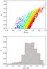 |
Fig. 1 CMD of the Galactic bulge in Baade’s window (30′ × 30′) in the selected upper RGB region, used for the interpolation routine. Stars are color coded acording to their individual metallicities. Lower panel shows the metallicity distribution for the same region, compared to that from high-resolution spectroscopy from Hill et al. (2011), shown in red. |
The complete method can be summarized as follows:
-
1.
The Ks0 luminosity functions are built for each VVV tile and the mean magnitude of the RC is calculated by fitting the equation
![\begin{equation} N(K_{\rm s_0})\!=\!a+bK_{\rm s_0}+cK_{\rm s_0}^2+\frac{N_{\rm RC}}{\sigma_{\rm RC}\sqrt{2\pi}}\exp\left[-\frac{(K_{\rm s_0}^{\rm RC}-K_{\rm s_0})^2}{2\sigma^2_{\rm RC}}\right]\cdot \end{equation}](/articles/aa/full_html/2013/04/aa20842-12/aa20842-12-eq25.png) (2)
(2) -
2.
Each tile is divided in four subfields of 30′ × 45′. The distance modulus is then derived for each subfield by (Ks,0 − MKs)RC using Eq. (1). In the first step, ΔMKs = 0, but this value changes in subsequent iterations.
-
3.
The (J − Ks)0 vs. MKs CMD for each 30′ × 45′ subfield is used to select stars with MKs > −4.5 and (J − Ks)0 > 0.65, selecting the RGB region above the asymptotic giant branch (AGB) bump that is more sensitive to metallicity and avoiding most of the foreground disk contamination. An upper magnitude cut is also applied at the MKs corresponding to the RGB tip measurements of bulge globular clusters from Valenti et al. (2007).
-
4.
The color of each star is then interpolated among the empirical templates of Galactic halo and bulge globular clusters (M 92, M 55, NGC 6752, NGC 362, M 69, NGC 6440, NGC 6528, and NGC 6791), with well-known metallicity, selected from the sample of Valenti et al. (2007). An individual metallicity value is obtained for the stars in each subfield by this color interpolation.
-
5.
The mean metallicity of the subfield is then obtained and the ΔMKs value is calculated using the new mean metallicity, which is based on Salaris & Girardi (2002) equation:
![\begin{equation} \Delta M_{K_{\rm s}}=0.275[{\rm Fe/H}]+1.496-M_{K_{\rm s}}(RC), \end{equation}](/articles/aa/full_html/2013/04/aa20842-12/aa20842-12-eq30.png) (3)and applied to Eq. (1).
(3)and applied to Eq. (1).
Steps 2−5 are iterated to obtain a final mean metallicity that corresponds to a single MKs. An example of the CMD in the Baade’s window, which is color coded by the metallicity of the individual stars, is shown in the upper panel of Fig. 1. The lower panel compares the photometric metallicities (hashed histogram) with the high-resolution spectroscopic measurements from Hill et al. (2011), which are presented in red.
Having proven the reliability of the mean metallicity measurements from the VVV+2MASS photometry (Paper I), we can now present in Fig. 2 the first global map of mean metallicity in bins of 30′ × 45′. This map is restricted to |b| > 3° as the upper RGB in our dataset corresponds to 2MASS photometry, which is limited by crowding in the inner regions. This is the first global view of the mean metallicity variations across the Milky Way bulge. The gradient along the minor axis, observed from high-resolution studies, is clearly seen in our map; it is the result of a central concentration of metal-rich stars in the region −5° < b < 5° and −7° < l < 7°. This concentration of near-solar metallicity stars seems to follow a radial gradient of ~0.04 dex/deg, going from more metal-poor stars in the outer bulge to more metal-rich stars towards the inner regions.
 |
Fig. 2 Map of the mean values of the metallicity distributions for the Galactic bulge covered by the VVV survey using the Cardelli extinction law. |
As described in Paper I, the metallicity map will be publicly available to the community via the Bulge Extinction And Metallicity (BEAM) calculator webpage1.
5. Sources of error
Clearly, the most accurate abundance measurements are obtained using high-resolution spectroscopic methods. Unfortunately, such studies are very expensive in terms of telescope time, allowing only a few regions to be studied and thus not enabling us to obtain a large-scale picture of the bulge chemical abundance properties. The accuracy of the photometric abundance derivations depends strongly on knowing other properties affecting the stellar population under study, such as the density distribution in the corresponding line of sight and the interstellar extinction. Although we have significantly improved our handling of the general properties of the bulge, such as distance spread and interstellar extinction, possible variations across different regions might still be present. Therefore, it is important to quantify the effect of such variations on our mean abundance determinations.
5.1. The bulge distance spread
Bulge stars are often assumed to be well represented by a population at ~8 kpc from the Sun (e.g., Rattenbury et al. 2007). However, for a wide field study such as the one presented here, we must include two factors into our analysis: the bar inclination angle and the distance spread of stars. As explained in Sect. 3, we have used the RC method to derive the mean distance of the stars towards each line of sight, so that the inclination angle of the bulge has been fully taken into consideration. However, by assuming that all stars are located at the same distance, corresponding to the distance modulus derived using the RC magnitude, we are introducing an error that is directly related to the magnitude width of the RC in the luminosity function.
The width of the RC luminosity function for a population located at the same distance will be determined by the intrinsic width given by properties such as metallicity and age. However, the dominant factor in the case of the bulge RC magnitude distribution width will be the distance spread. We have therefore used a boothstrapping method to estimate the uncertainty arising from adopting a single mean magnitude and neglecting the width of the bulge RC. We re-calculated the mean metallicity after varying the mean magnitude of the RC by a random value, which is within 2σ of the mean RC Ks magnitude. In each case, σ is obtained from the Gaussian fit to the luminosity function in Eq. (1). We repeated this procedure 600 times for each VVV tile, since one tile corresponds to our resolution element used to derive the mean RC magnitude. Figure 3 shows the dispersion (σdis) in the mean metallicity obtained for each VVV tile after the iteration procedure.
 |
Fig. 3 Metallicity dispersion σdis of each line of sight given by the individual VVV tiles, after varying the mean Ks magnitude for 600 random values within 2σ of the RC Gaussian fit. |
5.2. Residual differential extinction
Another source of uncertainties in our derivation of the mean metallicity is due to a possible presence of residual differential extinction. Although a great improvement is provided by the high-resolution extinction map presented in Gonzalez et al. (2012), the resolution of this map is limited because it requires a sufficient number of stars to fit the RC color distribution. The corresponding resolution of the map, under this limitation, was given by 2′, 4′, and 6′ arcmin, depending on latitude. Variations on scales smaller than these resolution elements are still possible, which then produce an increase in the width of the RC color and thus also in the RGB region that we use to derive the metallicities. As the reddening becomes larger towards the inner regions of the bulge, the residual reddening follows the same behavior. This creates an excess of redder stars in the CMD that would result in a derivation of higher photometric metallicities for those stars, creating a metallicity gradient like the one we observe in our maps. Thus, we must ensure that the gradient we observe is not a product of differential reddening but a real feature.
We therefore evaluate the effect of residual differential extinction by studying the width of the (J − Ks)0 color distribution of the RC, measured using a Gaussian fit to the RC color in each resolution element of the metallicity map. The dispersion, σ(J − Ks) of the Gaussian fit to RC color distribution will depend primarily on metallicity dispersion (σ(J − Ks),Fe), along with the presence of differential reddening (σ(J − Ks),red). We can thus parametrize σ(J − Ks) as  , where σ(J − Ks),0 is the uniform intrinsic width of the bulge RC population. In the context of this test, we can then adopt the hypothesis of having neither a metallicity nor a metallicity dispersion gradient in the bulge, where both σ(J − Ks),0 and σ(J − Ks),Fe can be assumed to be constant across the different regions and the single effect of residual differential extinction can be investigated. Then, under this assumption, the squared root difference between the σ(J − Ks) value in any region and that of the outermost region of our map, where the effects of extinction and residual reddening are not present, would be a direct measurment of σ(J − Ks),red. We calculated the σ(J − Ks),red values for each field using VVV field b217 as our reddening free control field.
Finally, we applied a 1σ(J − Ks),red variation to the color of the RGB stars of our control field in the outer bulge and re-derived the metallicity distribution for the σ(J − Ks),red corresponding to each field. Figure 4 shows the map of σFe,red given as the difference between the original [Fe/H] of the control field and the new value, affected by each σ(J − Ks),red. We observe that the residual differential reddening does not mask the shape of the metallicity gradient and, most importantly, the error values in metallicity due to differential reddening are almost negligible for most regions (less than 0.05).
 |
Fig. 4 Error in the mean metallicity derivation from residual differental reddening. Error values are given by the difference between the original [Fe/H] of the control field (b217) and the re-calculated metallicity after applying the σ(J − Ks),red corresponding to each field. |
5.3. Extinction law variations
The reddening E(J − Ks) from the map presented in Paper II can be converted to the extinctions AJ, AH, and AKs by adopting a corresponding extinction law. Most of the studies towards the Galactic bulge adopt standard extinction laws consistent with a RV ~ 3.1 (e.g., Cardelli et al. 1989). However, there are evidences for a non-standard extinction law, both in the optical and near-IR, towards the bulge. Gould et al. (2001) and Udalski (2003) demonstrated that the optical reddening law toward the inner Galaxy is described by smaller total-to-selective ratios than the standard values measured for the local interstellar medium. Udalski (2003) measured a value of dAI = dE(V − I) = 1.1 towards several bulge fields using Optical Gravitational Lensing Experiment (OGLE) photometry, much smaller than the dAI = dE(V − I) = 1.4 suggested by the standard interstellar extinction curve of RV = 3:1 (Cardelli et al. 1989; O’Donnell 1994). Furthermore, not only was the optical reddening law toward the bulge found to be non-standard, it was also determined to be rapidly varying between sightlines (Nataf et al. 2012). The steeper extinction law toward the inner Galaxy has been subsequently confirmed with observations in the optical (Revnivtsev et al. 2010) by analysis of RR Lyrae stars in OGLE-III (Pietrukowicz et al. 2012) and also in the near-IR (Nishiyama et al. 2009; Gosling et al. 2009; Schödel et al. 2010).
An error in our metallicity calculations can be produced by adopting an extinction law for the complete bulge region that is no longer be valid in all regions. In particular, if a difference in the extinction law is present between the outer and inner bulge, a metallicity gradient could also be a consequence of this systematic error instead of a real feature. Therefore, we derived our metallicity map using the standard law of Cardelli et al. (1989), shown in Fig. 2, and that of Nishiyama et al. (2009), which is shown in Fig. 5. The difference between the metallicity obtained using both reddening laws allows us to evaluate its effect on the observed gradient. Figure 6 shows the difference between the metallicity map derived using Cardelli et al. (1989) and that of Nishiyama et al. (2009). The maximum difference is observed to be of 0.10 dex in the mean metallicity and, as expected, correlates with the amount of extinction. The variations in extinction law are therefore not enough to produce the observed gradient and variations also do not follow the same spatial behavior of the metallicity gradient.
 |
Fig. 5 Metallicity map for the Galactic bulge, as shown in Fig. 2, using the extinction law from Nishiyama et al. (2009). |
 |
Fig. 6 Difference, [Fe/H] nishiyama − [Fe/H] cardelli, between the metallicities derived using the extinction law of Nishiyama et al. (2009) and that of Cardelli et al. (1989) for the Galactic bulge. |
Additionally, we can evaluate the possible effect of extinction law variations in our derived photometric metallicities. For this we must first assume that the metallicity distribution function is symmetric with respect to the Galactic plane. If this is the case, then the difference between metallicities measured at positive and negative latitudes should be zero. On the other hand, since the amount of reddening is not necessarily symmetric with respect to the plane and is observed to be higher at positive latitudes than at negative ones (Marshall et al. 2006; Gonzalez et al. 2012), an asymmetric metallicity map would result if reddening and metallicity are not properly disentagled because of, for example, the use of a non-suitable extinction law. Figure 7 shows the mean difference found between metallicities above (b > 0) and below (b < 0) the Galactic plane as a function of distance from the plane. Error bars show the dispersion in this difference in metallicity for each latitude bin.
 |
Fig. 7 Difference in the mean metallicity at different latitudes above ([Fe/H]+) and below ([Fe/H]−) the Galactic plane. The mean difference is shown as a dotted line. Results obtained using the Cardelli et al. (1989) extinction law (black line) and the Nishiyama et al. (2009) law (red line) is adopted. |
We found a small systematic shift from zero (Δ[Fe/H] ~ −0.01) in the mean metallicity difference when using the Cardelli et al. (1989) extinction law, which is no longer present when the Nishiyama et al. (2009) law is adopted. This particular analysis would be independent of the adopted extinction law only if the amount of reddening was the same at both positive and negative latitudes. Therefore, we can interpret this result as the combined effect of the large amount of reddening at positive latitudes and the Cardelli et al. law being less adequate to correct for extinction effects in these inner bulge regions. This effect is already included in our previously estimated errors for each resolution element of our metallicity map, but we can now confirm the actual improvement of using the Nishiyama et al. (2009) extinction law in the inner bulge regions (b < 5).
5.4. The metallicity error map
After evaluating the individual sources of errors from the distance uncertainty, differential reddening, and the extinction law, we obtain a map with the corresponding error for each of the subfields in our metallicity map, calculated as:  (4)Figure 8 shows the error metallicity map for each subfield. This error does not include the method error associated to obtain photometric metallicities. Although the individual errors of photometric metallicities are expected to be larger than those from spectroscopy, we see differences lower than 0.05 dex between high-resolution spectroscopic and photometric metallicities when the mean value of the metallicity distribution is considered. We therefore consider this method error in the mean to be negligible compared to those previously addressed.
 |
Fig. 8 Error map for the mean photometric metallicity for each subfield. |
6. The formation scenario of the bulge
In recent years, several authors have suggested that the shape of the metallicity distribution and its variation across the bulge is determined by the different contributions of two (or more) components. However, the origin of these components and their main characteristics, such as their age and metallicity, are not yet clear. Therefore, the complete view of the metallicity gradients accross the bulge is of high importance for constraining Galactic models.
The presence of a radial metallicity gradient is commonly considered a strong argument in favor of the classical bulge scenario. In our complete metallicity map, we observe such a gradient: a [Fe/H] ~ 0.28 dex/kpc, a value that is in remarkable agreement with the predicted gradient for bulge formed via dissipational collapse in the chemo-dynamical model discussed in Grieco et al. (2012).
However, structural and kinematical studies indicate a different scenario. There is sufficient evidence that the Milky Way bulge structure is consistent with a boxy bulge, formed as a consequence of the vertical buckling of the bar. Several photometric studies have shown how the bar can be traced at latitudes well above the Galactic plane (Stanek et al. 1997; López-Corredoira et al. 2005; Rattenbury et al. 2007; Dwek et al. 1995; Binney et al. 1997). Plane studies of the bar, in particular those based on near-IR star counts, have suggested the presence of a longer bar in the plane of the Milky Way, which extends to larger longitudes and has a different orientation angle than the off-plane bar (Benjamin et al. 2005; Cabrera-Lavers et al. 2007, 2008; Churchwell et al. 2009). Martinez-Valpuesta & Gerhard (2011) have recently presented a dynamical model where a bar and boxy bulge are formed through secular evolution, conciliating both long- and thick-bar components observed in the Milky Way into a single original structure. Additionally, the cylindrical rotation of this structure led Shen et al. (2010) to suggest that no additional classical component is required to reproduce the Milky Way bulge kinematical properties. Furthermore, McWilliam & Zoccali (2010) and Nataf et al. (2010) presented the observations of a double RC feature in the luminosity function of the bulge and interpreted it as two concentration of stars at different distances. McWilliam & Zoccali (2010) suggested that this is the result of the bulge being X-shaped. This finding was later followed by a more complete mapping of the double RC in the work of Saito et al. (2011), who provided a more general view of the X-shape morphology of the bulge.
These conclusions regarding the morphology and kinematics of the Galactic bulge are consistent with results from simulations where a bar suffering from buckling instabilities results in the formation of a peanut or X-shaped structure (Athanassoula 2005; Debattista & Williams 2004; Debattista et al. 2006; Martinez-Valpuesta et al. 2006) that puffs up from the plane of the galaxy. When these vertically thickened bars are observed with an intermediate angle orientation, they would appear as boxy bulges (Kuijken & Merrifield 1995; Bureau & Freeman 1999; Patsis et al. 2002; Bureau et al. 2006). Additionally, we see from the metallicity map in Fig. 2 that stars at larger latitudes are more metal-rich at positive longitudes than at to negative ones. Following the discussion in Saito et al. (2011), at a given latitude, stars at negative longitudes are farther away from us because of the bar-viewing angle. Therefore, their true vertical distance from the plane will be larger than for stars at the near side of the bar. The observed horizontal pattern in the metallicity map of Fig. 2 would then be fully explained by the vertical metallicity gradient along the boxy bulge.
In order to reconcile these chemical and structural properties of the Galactic bulge, we first need to understand whether boxy bulges alone can also show a metallicity gradient such as the one observed in our map. Bekki & Tsujimoto (2011) discussed this possibility, based on a Galactic model where a boxy bulge is formed out of a two-component disk. In their simulation, they are able to reproduce a vertical metallicity gradient when the bulge is secularly born from an original disk with its own vertical metallicity gradient, i.e., a metal-poor thick- and metal-rich thin-disk component, such as those observed in the Milky Way. The initial chemical properties of the stars in the disk would then produce the observed metallicity gradient, since the metal-poor stars that dominate the dynamically hotter thick disk would not be influenced by the mixing within the bar.
The boxy bulge model of Martinez-Valpuesta & Gerhard (2011), which has been shown to succesfully reproduce the stellar count profiles for both the inner and outer bulge, also demonstrates a remarkable agreement with the complete metallicity gradient presented in this work (Martinez-Valpuesta & Gerhard 2013). We recall that the model does not include a classical component, hence demonstrating that the buckling process of a secularly evolved bar could be sufficient to explain the formation history of the bulge.
In support of the above scenario, there is the chemical similarity observed between bulge and disk stars. Metal-rich stars of the bulge are observed to be as alpha-poor as those of the thin disk, while metal-poor bulge stars show an alpha-element enhancement that is indistinguishable from that of the Galactic thick disk and dominates at higher scale heights (Meléndez et al. 2008; Alves-Brito et al. 2010; Gonzalez et al. 2011a). Furthermore, the mainly old stellar ages observed in the bulge (Zoccali et al. 2003; Clarkson et al. 2011) place additional constraints on such formation scenarios. The original thick disk would have to have formed fast (~1 Gyr), most likely as the result of dissipative collapse or the merging of gas-rich subgalactic clumps, in order to be consistent with the early formation of the hotter, old, and alpha-enhanced component. The inner stellar disk would then need to proceed with its star formation, relatively fast compared to the outer thin disk, to become the inner parts of the boxy bulge.
Finally, we recall that recent studies have also suggested that the chemodynamical properties of the bulge are consistent with a change of the dominating population between the outer and inner bulge: a metal-poor, alpha-rich component with spheroid kinematics that is homogeneous along the minor axis and a metal-rich, alpha-poor bar population that dominates the inner bulge (Babusiaux et al. 2010; Hill et al. 2011; Gonzalez et al. 2011a). Under this interpretation, the vertical metallicity gradient will be naturally produced by the density distribution of both components at different lines of sight. Although this is also consistent with the general view seen in our complete metallicity map, the large individual metallicity errors in our photometric method in comparison to those from spectroscopy do not allow further investigation of the bimodality in the metallicity distribution (see Fig. 1). Therefore, the presence of a bimodal metallicity distribution and its correlation with kinematics remains to be spectroscopically confirmed within a large spatial coverage.
7. Conclusions
We used the RC stars of the Galactic bulge as a standard candle to build a reddening map and determine distances. This allowed us to construct the CMDs of bulge stars in the absolute plane (MKs,(J − Ks)0) and then to obtain individual photometric metallicities for RGB stars in the bulge through interpolation on the RGB ridge lines of cluster sample from Valenti et al. (2007), taking into account the population corrections for the RC absolute magnitude as a function of metallicity in an iterative procedure. The final metallicity distributions were compared to those obtained in the spectroscopic studies and showed a remarkable agreement. The main result is the first high-resolution metallicity map of the Milky Way bulge with a global coverage from −10 < l < +10 and −10 < b < +5, excluding the central area (|b| < 2), where too high crowding and strong differential extinction compromise the measurements.
The global bulge metallicity map is consistent with a vertical metallicity gradient (~0.04 dex/deg), with metal-rich stars ([Fe/H] ~ 0) dominating the inner bulge in regions closer to the Galactic plane (|b| < 5). At larger scale heights, the mean metallicity of the bulge population becomes more metal-poor. This fits in the scenario of older, metal-poor stars dominating the bulge at higher scale heights above the plane as a consequence of original gradients present in the Galactic disk. Therefore, our metallicity map supports the formation of the boxy bulge from the buckling instabillity of the Galactic bar (Bekki & Tsujimoto 2011; Martinez-Valpuesta & Gerhard 2011). This scenario is also supported by the chemical similarities observed between the metal-poor bulge and the thick-disk stars.
Acknowledgments
We thank the referee, David Nataf, for a careful review and valuable comments that contributed to the improvement of the article. We warmly thank Alvio Renzini and Vanessa Hill for providing useful comments and suggestions to this work. We are grateful to Inma Martinez-Valpuesta and Ortwin Gerhard for sharing their model results before publication. We gratefully acknowledge use of data from the ESO Public Survey program ID 179.B-2002 taken with the VISTA telescope and data products from the Cambridge Astronomical Survey Unit. We acknowledge funding from the FONDAP Center for Astrophysics 15010003, the BASAL CATA Center for Astrophysics and Associated Technologies PFB-06, the MILENIO Milky Way Millennium Nucleus from the Ministry of Economycs ICM grant P07-021-F and Proyectos FONDECYT Regular 1110393 and 1090213. M.Z. is also partially supported by Proyecto Anillo ACT-86. This work was co-funded under the Marie Curie Actions of the European Commission (FP7-COFUND). It uses data products from the Two Micron All Sky Survey, which is a joint project of the University of Massachusetts and Infrared Processing and Analysis Center/California Institute of Technology, funded by the National Aeronautics and Space Administration and the National Science Foundation. We warmly thank the ESO Paranal Observatory staff for performing the observations.
References
- Alves-Brito, A., Meléndez, J., Asplund, M., Ramírez, I., & Yong, D. 2010, A&A, 513, A35 [NASA ADS] [CrossRef] [EDP Sciences] [Google Scholar]
- Athanassoula, E. 2005, MNRAS, 358, 1477 [NASA ADS] [CrossRef] [Google Scholar]
- Athanassoula, E., & Misiriotis, A. 2002, MNRAS, 330, 35 [NASA ADS] [CrossRef] [Google Scholar]
- Babusiaux, C., Gómez, A., Hill, V., et al. 2010, A&A, 519, A77 [NASA ADS] [CrossRef] [EDP Sciences] [Google Scholar]
- Bekki, K., & Tsujimoto, T. 2011, MNRAS, 416, L60 [NASA ADS] [CrossRef] [Google Scholar]
- Benjamin, R. A., Churchwell, E., Babler, B. L., et al. 2005, ApJ, 630, L149 [NASA ADS] [CrossRef] [Google Scholar]
- Bensby, T., Feltzing, S., Gould, A., et al. 2012, in Galactic Archaeology: Near-Field Cosmology and the Formation of the Milky Way, eds. W. Aoki, M. Ishigaki, T. Suda, T. Tsujimoto, & N. Arimoto, ASP Conf. Ser., 458, 203 [Google Scholar]
- Binney, J., Gerhard, O., & Spergel, D. 1997, MNRAS, 288, 365 [NASA ADS] [CrossRef] [Google Scholar]
- Bureau, M., & Freeman, K. C. 1999, AJ, 118, 126 [NASA ADS] [CrossRef] [Google Scholar]
- Bureau, M., Aronica, G., Athanassoula, E., et al. 2006, MNRAS, 370, 753 [NASA ADS] [CrossRef] [Google Scholar]
- Cabrera-Lavers, A., Hammersley, P. L., González-Fernández, C., et al. 2007, A&A, 465, 825 [NASA ADS] [CrossRef] [EDP Sciences] [Google Scholar]
- Cabrera-Lavers, A., González-Fernández, C., Garzón, F., Hammersley, P. L., & López-Corredoira, M. 2008, A&A, 491, 781 [NASA ADS] [CrossRef] [EDP Sciences] [Google Scholar]
- Cardelli, J. A., Clayton, G. C., & Mathis, J. S. 1989, ApJ, 345, 245 [NASA ADS] [CrossRef] [Google Scholar]
- Carollo, C. M., Scarlata, C., Stiavelli, M., Wyse, R. F. G., & Mayer, L. 2007, ApJ, 658, 960 [NASA ADS] [CrossRef] [Google Scholar]
- Churchwell, E., Babler, B. L., Meade, M. R., et al. 2009, PASP, 121, 213 [NASA ADS] [CrossRef] [Google Scholar]
- Clarkson, W. I., Sahu, K. C., Anderson, J., et al. 2011, ApJ, 735, 37 [NASA ADS] [CrossRef] [Google Scholar]
- Combes, F., & Sanders, R. H. 1981, A&A, 96, 164 [NASA ADS] [Google Scholar]
- Combes, F., Debbasch, F., Friedli, D., & Pfenniger, D. 1990, A&A, 233, 82 [NASA ADS] [Google Scholar]
- Daddi, E., Bournaud, F., Walter, F., et al. 2010, ApJ, 713, 686 [NASA ADS] [CrossRef] [Google Scholar]
- Debattista, V. P., & Sellwood, J. A. 1998, ApJ, 493, L5 [NASA ADS] [CrossRef] [Google Scholar]
- Debattista, V. P., & Williams, T. B. 2004, ApJ, 605, 714 [NASA ADS] [CrossRef] [Google Scholar]
- Debattista, V. P., Mayer, L., Carollo, C. M., et al. 2006, ApJ, 645, 209 [NASA ADS] [CrossRef] [Google Scholar]
- Dwek, E., Arendt, R. G., Hauser, M. G., et al. 1995, ApJ, 445, 716 [CrossRef] [Google Scholar]
- Elmegreen, B. G., Bournaud, F., & Elmegreen, D. M. 2008, ApJ, 688, 67 [NASA ADS] [CrossRef] [Google Scholar]
- Emsellem, E., Cappellari, M., Peletier, R. F., et al. 2004, MNRAS, 352, 721 [NASA ADS] [CrossRef] [Google Scholar]
- Eskridge, P. B., Frogel, J. A., Pogge, R. W., et al. 2000, AJ, 119, 536 [NASA ADS] [CrossRef] [Google Scholar]
- FörsterSchreiber, N. M., Genzel, R., Bouché, N., et al. 2009, ApJ, 706, 1364 [NASA ADS] [CrossRef] [Google Scholar]
- Freeman, K. C. 2008, in IAU Symp. 245, eds. M. Bureau, E. Athanassoula, & B. Barbuy, 3 [Google Scholar]
- Gadotti, D. A. 2009, MNRAS, 393, 1531 [NASA ADS] [CrossRef] [Google Scholar]
- Gadotti, D. A. 2012, Astron. Astrophys. Trans., 27, 221 [NASA ADS] [Google Scholar]
- Gadotti, D. A., & de Souza, R. E. 2006, ApJS, 163, 270 [NASA ADS] [CrossRef] [Google Scholar]
- Genzel, R., Tacconi, L. J., Eisenhauer, F., et al. 2006, 442, 786 [Google Scholar]
- Genzel, R., Burkert, A., Bouché, N., et al. 2008, ApJ, 687, 59 [NASA ADS] [CrossRef] [Google Scholar]
- Gonzalez, O. A., Rejkuba, M., Zoccali, M., et al. 2011a, A&A, 530, A54 [NASA ADS] [CrossRef] [EDP Sciences] [Google Scholar]
- Gonzalez, O. A., Rejkuba, M., Zoccali, M., Valenti, E., & Minniti, D. 2011b, A&A, 534, A3 [NASA ADS] [CrossRef] [EDP Sciences] [Google Scholar]
- Gonzalez, O. A., Rejkuba, M., Zoccali, M., et al. 2012, A&A, 543, A13 [NASA ADS] [CrossRef] [EDP Sciences] [Google Scholar]
- Gosling, A. J., Bandyopadhyay, R. M., & Blundell, K. M. 2009, MNRAS, 394, 2247 [NASA ADS] [CrossRef] [Google Scholar]
- Gould, A., Stutz, A., & Frogel, J. A. 2001, ApJ, 547, 590 [NASA ADS] [CrossRef] [Google Scholar]
- Grieco, V., Matteucci, F., Pipino, A., & Cescutti, G. 2012, A&A, 548, A60 [NASA ADS] [CrossRef] [EDP Sciences] [Google Scholar]
- Hill, V., Lecureur, A., Gomez, A., et al. 2011, A&A, 534, A80 [NASA ADS] [CrossRef] [EDP Sciences] [Google Scholar]
- Immeli, A., Samland, M., Gerhard, O., & Westera, P. 2004, A&A, 413, 547 [NASA ADS] [CrossRef] [EDP Sciences] [Google Scholar]
- Jablonka, P., & Sarajedini, A. 2005, in From Lithium to Uranium: Elemental Tracers of Early Cosmic Evolution, eds. V. Hill, P. François, & F. Primas, IAU Symp., 228, 525 [Google Scholar]
- Jablonka, P., Gorgas, J., & Goudfrooij, P. 2007, A&A, 474, 763 [NASA ADS] [CrossRef] [EDP Sciences] [Google Scholar]
- Johnson, C. I., Rich, R. M., Fulbright, J. P., Valenti, E., & McWilliam, A. 2011, ApJ, 732, 108 [NASA ADS] [CrossRef] [Google Scholar]
- Kauffmann, G., Colberg, J. M., Diaferio, A., & White, S. D. M. 1999, MNRAS, 303, 188 [NASA ADS] [CrossRef] [Google Scholar]
- Kormendy, J., & Bruzual, A. G. 1978, ApJ, 223, L63 [NASA ADS] [CrossRef] [Google Scholar]
- Kormendy, J., & Illingworth, G. 1982, ApJ, 256, 460 [NASA ADS] [CrossRef] [Google Scholar]
- Kormendy, J., & Kennicutt, Jr., R. C. 2004, 42, 603 [Google Scholar]
- Kuijken, K., & Merrifield, M. R. 1995, ApJ, 443, L13 [NASA ADS] [CrossRef] [Google Scholar]
- López-Corredoira, M., Cabrera-Lavers, A., & Gerhard, O. E. 2005, A&A, 439, 107 [NASA ADS] [CrossRef] [EDP Sciences] [Google Scholar]
- MacArthur, L. A., Ellis, R. S., Treu, T., et al. 2008, ApJ, 680, 70 [NASA ADS] [CrossRef] [Google Scholar]
- Marshall, D. J., Robin, A. C., Reylé, C., Schultheis, M., & Picaud, S. 2006, A&A, 453, 635 [NASA ADS] [CrossRef] [EDP Sciences] [Google Scholar]
- Martinez-Valpuesta, I., & Gerhard, O. 2011, ApJ, 734, L20 [NASA ADS] [CrossRef] [Google Scholar]
- Martinez-Valpuesta, I., & Gerhard, O. 2013, ApJ, accepted [arXiv:1302.1613] [Google Scholar]
- Martinez-Valpuesta, I., Shlosman, I., & Heller, C. 2006, ApJ, 637, 214 [NASA ADS] [CrossRef] [Google Scholar]
- McWilliam, A., & Zoccali, M. 2010, ApJ, 724, 1491 [NASA ADS] [CrossRef] [Google Scholar]
- Meléndez, J., Asplund, M., Alves-Brito, A., et al. 2008, A&A, 484, L21 [NASA ADS] [CrossRef] [EDP Sciences] [MathSciNet] [Google Scholar]
- Minniti, D., Lucas, P. W., Emerson, J. P., et al. 2010, 15, 433 [Google Scholar]
- Moorthy, B. K., & Holtzman, J. A. 2006, MNRAS, 371, 583 [NASA ADS] [CrossRef] [Google Scholar]
- Nataf, D. M., Gould, A., Fouqué, P., et al. 2012, ApJ, submitted [arXiv:1208.1263] [Google Scholar]
- Nataf, D. M., Udalski, A., Gould, A., Fouqué, P., & Stanek, K. Z. 2010, ApJ, 721, L28 [NASA ADS] [CrossRef] [Google Scholar]
- Ness, M., Freeman, K., Athanassoula, E., et al. 2012, ApJ, 756, 22 [NASA ADS] [CrossRef] [Google Scholar]
- Nishiyama, S., Tamura, M., Hatano, H., et al. 2009, ApJ, 696, 1407 [NASA ADS] [CrossRef] [Google Scholar]
- O’Donnell, J. E. 1994, ApJ, 422, 158 [NASA ADS] [CrossRef] [Google Scholar]
- Patsis, P. A., Skokos, C., & Athanassoula, E. 2002, MNRAS, 337, 578 [NASA ADS] [CrossRef] [Google Scholar]
- Peletier, R. F., Balcells, M., Davies, R. L., et al. 1999, MNRAS, 310, 703 [NASA ADS] [CrossRef] [Google Scholar]
- Peng, Y., Lilly, S. J., Kovač, K., et al. 2010, ApJ, 721, 193 [NASA ADS] [CrossRef] [Google Scholar]
- Pérez, I., Sánchez-Blázquez, P., & Zurita, A. 2009, A&A, 495, 775 [NASA ADS] [CrossRef] [EDP Sciences] [Google Scholar]
- Pietrinferni, A., Cassisi, S., Salaris, M., & Castelli, F. 2004, ApJ, 612, 168 [NASA ADS] [CrossRef] [Google Scholar]
- Pietrukowicz, P., Udalski, A., Soszyński, I., et al. 2012, ApJ, 750, 169 [NASA ADS] [CrossRef] [Google Scholar]
- Rattenbury, N. J., Mao, S., Sumi, T., & Smith, M. C. 2007, MNRAS, 378, 1064 [NASA ADS] [CrossRef] [Google Scholar]
- Renzini, A. 1998, AJ, 115, 2459 [Google Scholar]
- Renzini, A. 2009, MNRAS, 398, L58 [NASA ADS] [Google Scholar]
- Revnivtsev, M., van den Berg, M., Burenin, R., et al. 2010, A&A, 515, A49 [NASA ADS] [CrossRef] [EDP Sciences] [Google Scholar]
- Rich, R. M., Origlia, L., & Valenti, E. 2007, ApJ, 665, L119 [NASA ADS] [CrossRef] [Google Scholar]
- Saito, R. K., Zoccali, M., McWilliam, A., et al. 2011, AJ, 142, 76 [NASA ADS] [CrossRef] [Google Scholar]
- Saito, R. K., Hempel, M., Minniti, D., et al. 2012, A&A, 537, A107 [NASA ADS] [CrossRef] [EDP Sciences] [Google Scholar]
- Salaris, M., & Girardi, L. 2002, MNRAS, 337, 332 [NASA ADS] [CrossRef] [Google Scholar]
- Schödel, R., Najarro, F., Muzic, K., & Eckart, A. 2010, A&A, 511, A18 [NASA ADS] [CrossRef] [EDP Sciences] [Google Scholar]
- Shen, J., Rich, R. M., Kormendy, J., et al. 2010, ApJ, 720, L72 [NASA ADS] [CrossRef] [Google Scholar]
- Springel, V., & Hernquist, L. 2005, ApJ, 622, L9 [NASA ADS] [CrossRef] [Google Scholar]
- Stanek, K. Z., Udalski, A., Szymanski, M., et al. 1997, ApJ, 477, 163 [NASA ADS] [CrossRef] [Google Scholar]
- Tacconi, L. J., Genzel, R., Neri, R., et al. 2010, 463, 781 [Google Scholar]
- Toomre, A. 1977, 15, 437 [Google Scholar]
- Udalski, A. 2003, ApJ, 590, 284 [NASA ADS] [CrossRef] [Google Scholar]
- Uttenthaler, S., Schultheis, M., Nataf, D. M., et al. 2012, A&A, 546, A57 [NASA ADS] [CrossRef] [EDP Sciences] [Google Scholar]
- Valenti, E., Ferraro, F. R., & Origlia, L. 2007, AJ, 133, 1287 [NASA ADS] [CrossRef] [Google Scholar]
- van Helshoecht, V., & Groenewegen, M. A. T. 2007, A&A, 463, 559 [NASA ADS] [CrossRef] [EDP Sciences] [Google Scholar]
- Weinberg, M. D. 1985, MNRAS, 213, 451 [NASA ADS] [CrossRef] [Google Scholar]
- Zoccali, M., Renzini, A., Ortolani, S., et al. 2003, A&A, 399, 931 [NASA ADS] [CrossRef] [EDP Sciences] [Google Scholar]
- Zoccali, M., Hill, V., Lecureur, A., et al. 2008, A&A, 486, 177 [NASA ADS] [CrossRef] [EDP Sciences] [Google Scholar]
All Figures
|
Fig. 1 CMD of the Galactic bulge in Baade’s window (30′ × 30′) in the selected upper RGB region, used for the interpolation routine. Stars are color coded acording to their individual metallicities. Lower panel shows the metallicity distribution for the same region, compared to that from high-resolution spectroscopy from Hill et al. (2011), shown in red. |
| In the text | |
|
Fig. 2 Map of the mean values of the metallicity distributions for the Galactic bulge covered by the VVV survey using the Cardelli extinction law. |
| In the text | |
|
Fig. 3 Metallicity dispersion σdis of each line of sight given by the individual VVV tiles, after varying the mean Ks magnitude for 600 random values within 2σ of the RC Gaussian fit. |
| In the text | |
|
Fig. 4 Error in the mean metallicity derivation from residual differental reddening. Error values are given by the difference between the original [Fe/H] of the control field (b217) and the re-calculated metallicity after applying the σ(J − Ks),red corresponding to each field. |
| In the text | |
|
Fig. 5 Metallicity map for the Galactic bulge, as shown in Fig. 2, using the extinction law from Nishiyama et al. (2009). |
| In the text | |
|
Fig. 6 Difference, [Fe/H] nishiyama − [Fe/H] cardelli, between the metallicities derived using the extinction law of Nishiyama et al. (2009) and that of Cardelli et al. (1989) for the Galactic bulge. |
| In the text | |
|
Fig. 7 Difference in the mean metallicity at different latitudes above ([Fe/H]+) and below ([Fe/H]−) the Galactic plane. The mean difference is shown as a dotted line. Results obtained using the Cardelli et al. (1989) extinction law (black line) and the Nishiyama et al. (2009) law (red line) is adopted. |
| In the text | |
|
Fig. 8 Error map for the mean photometric metallicity for each subfield. |
| In the text | |
Current usage metrics show cumulative count of Article Views (full-text article views including HTML views, PDF and ePub downloads, according to the available data) and Abstracts Views on Vision4Press platform.
Data correspond to usage on the plateform after 2015. The current usage metrics is available 48-96 hours after online publication and is updated daily on week days.
Initial download of the metrics may take a while.