| Issue |
A&A
Volume 552, April 2013
|
|
|---|---|---|
| Article Number | A131 | |
| Number of page(s) | 16 | |
| Section | Stellar structure and evolution | |
| DOI | https://doi.org/10.1051/0004-6361/201220726 | |
| Published online | 16 April 2013 | |
Population II stars and the Spite plateau
Stellar evolution models with mass loss⋆
1 LUPM, Université Montpellier II, CNRS CC072Place E. Bataillon 34095 Montpellier Cedex France
e-mail: This email address is being protected from spambots. You need JavaScript enabled to view it.
2 LUTH, Observatoire de Paris, CNRS, Université Paris Diderot, 5 place Jules Janssen, 92190 Meudon, France
3 Département de physique, Université de Montréal, Montréal, Québec, H3C 3J7, Canada
e-mail: This email address is being protected from spambots. You need JavaScript enabled to view it.
; This email address is being protected from spambots. You need JavaScript enabled to view it.
, This email address is being protected from spambots. You need JavaScript enabled to view it.
Received: 12 November 2012
Accepted: 22 February 2013
Abstract
Aims. We aim to determine the constraints that observed chemical abundances put on the potential role of mass loss in metal poor dwarfs.
Methods. Self-consistent stellar evolutionary models that include all the effects of atomic diffusion and radiative accelerations for 28 chemical species were computed for stellar masses between 0.6 and 0.8 M⊙. Models with an initial metallicity of Z0 = 0.00017 and mass loss rates from 10-15 M⊙ yr-1 to 10-12 M⊙ yr-1 were calculated. They were then compared to previous models with mass loss, as well as to models with turbulent mixing.
Results. For models with an initial metallicity of [Fe/H]0 = −2.31, mass loss rates of about 10-12 M⊙ yr-1 lead to surface abundance profiles that are very similar to those obtained in models with turbulence. Both models have about the same level of agreement with observations of galactic-halo lithium abundances, as well as lithium and other elemental abundances from metal poor globular clusters such as NGC 6397. In this cluster, models with mass loss agree slightly better with subgiant observations of Li abundance than those with turbulence. Lower red giant branch stars instead favor the models with turbulence. Larger differences between models with mass loss and those with turbulence appear in the interior concentrations of metals.
Conclusions. The relatively high mass loss rates required to reproduce plateau-like lithium abundances appear unlikely when compared to the solar mass-loss rate. However the presence of a chromosphere on these stars justifies further investigation of the mass-loss rates.
Key words: diffusion / stars: abundances / stars: interiors / stars: Population II / stars: mass-loss
Appendix A is available in electronic form at http://www.aanda.org
© ESO, 2013
1. Astrophysical context
Population II stars can be used as tracers for exploring the universe’s chemical evolution. Still, to correctly relate the chemical properties of the early Universe to the composition of the oldest observed stars, one must be able to map the evolution of their current abundances back to their original values. Doing so could help elucidate numerous questions pertaining to Big Bang nucleosynthesis, the nature of the first supernovae, and the age of the Universe.
The nearly constant Li abundance of most low-metallicity ([Z/H] < − 1.5) halo field stars whose Teff is between 6300 K and 5500 K – otherwise known as the Spite plateau (Spite & Spite 1982; Spite et al. 1984) – has puzzled astronomers for decades. Originally, many inferred that this plateau was representative of the Universe’s original Li abundance, though it was promptly shown that this could not be the case (Michaud et al. 1984). Precise observations of the cosmic microwave background1 have now led to a primordial lithium abundance2 of  , or even higher,
  (Cyburt et al. 2003, 2008; Steigman 2007), while the lithium content in metal poor dwarfs, ranging from A(7Li) = 2.0 to 2.4 is a factor of 2−3 lower (Bonifacio et al. 2007; Asplund et al. 2006; Charbonnel & Primas 2005; Meléndez & Ramírez 2004; Bonifacio 2002; Ryan et al. 1999).
Changing the standard Big Bang nucleosynthesis model is a possible explanation, though it is hypothetical (Ichikawa et al. 2004; Coc et al. 2004; Cumberbatch et al. 2007; Regis & Clarkson 2012). Even though Population III stars may have destroyed some of the primordial lithium (Piau et al. 2006), this cannot explain the large discrepancy. This leads many to assume that the solution stems from within the stars themselves. Possible stellar explanations may include destruction via gravity waves (Talon & Charbonnel 2004; Charbonnel & Talon 2005), and rotational mixing (Vauclair 1988; Charbonnel et al. 1992; Pinsonneault et al. 1999), as well as settling via atomic diffusion (Deliyannis et al. 1990; Profitt & Michaud 1991; Salaris et al. 2000; Richard et al. 2005). A higher Li content of subgiant (SG) stars compared to main–sequence (MS) stars in globular clusters (GC) such as NGC 6397 (Korn et al. 2007; Lind et al. 2009) favors a model in which lithium is not destroyed, but simply sunk below the photosphere prior to dredge-up. This result is, however, sensitive to the Teff scale used (González Hernández et al. 2009; Nordlander et al. 2012).
Additional constraints may stem from claimed observations of 6Li (Asplund et al. 2006), which, with a thermonuclear destruction cross section 60 times larger than the heavier isotope, would severely constrain the stellar destruction of 7Li. These observations remain very uncertain (Cayrel et al. 2007; Lind et al. 2012). Many recent studies have also claimed that below [Fe/H]≃ − 2.5, Li abundances lie significantly below the Spite plateau abundance and with increased scatter (Asplund et al. 2006; Aoki et al. 2009; Sbordone et al. 2010, 2012). Other observations suggest that there might instead be a lower plateau abundance for extremely metal poor (EMP) stars (Meléndez et al. 2010). The situation is complex and not currently understood in detail.
Although the surface convection zone (SCZ) of galactic Population II stars homogenizes abundances down to depths at which atomic diffusion is relatively slow, the long lifetimes of these stars, which reach the age of the Universe, allows for the effects of chemical separation to materialize at the surface. However, models that allow atomic diffusion to take place unimpeded lead to lithium underabundances that are too large at the hot end of the plateau (Michaud et al. 1984). By enforcing additional turbulent mixing below the SCZ, models of metal poor stars with gravitational settling and radiative accelerations are able to reproduce many observations of halo and globular cluster stars (Richard et al. 2002a,b, 2005; VandenBerg et al. 2002; Korn et al. 2006). These same models were also successful in explaining abundance anomalies in AmFm (Richer et al. 2000, 2001) and horizontal branch stars (Michaud et al. 2007, 2008).
In Vauclair & Charbonnel (1995), gravitational settling is inhibited by unseparated mass loss at the constant rate of ~3 × 10-13 M⊙ yr-1; this leads to near constant lithium abundances as a function of Teff, even at the hot end of the plateau. However, these calculations, which are discussed in Sect. 4, did not include the effects of radiative accelerations, nor did they follow atomic diffusion in detail for elements heavier than Li; therefore, further inspection is warranted.
In Vick et al. (2010, 2011), hereafter Papers I and II, stellar evolution models with mass loss were introduced and shown to reproduce observed surface abundance anomalies for many AmFm and chemically anomalous HAeBe binary stars. In Michaud et al. (2011) it was then shown that a mass loss rate compatible with the observed Sirius A mass loss rate leads to abundance anomalies similar to those observed on Sirius A. To further validate the model and to help constrain the relative importance of mass loss with respect to turbulent mixing in stars, the present mass loss models will be applied to Pop II stars and compared to models with turbulence from Richard et al. (2002b, 2005), which are able to reproduce observations of galactic halo stars, as well as of globular cluster stars on the subgiant and giant branches.
In the following analysis and in our calculations, mass loss is considered in non rotating stars, since in these stars it might be the only process competing with atomic diffusion. To our knowledge, mass loss has never been observed in Population II MS stars; therefore, mass loss rates will be constrained solely via surface abundance anomalies. In Sect. 2, the evolutionary calculations are presented, while the results are discussed in Sect. 3. In Sects. 4 and 5, the models with mass loss are compared to previous evolutionary models of metal poor dwarfs with mass loss, as well as to models with turbulence. In Sect. 6 results are compared to subgiant and giants both for models with turbulence and with mass loss. Conclusions follow in Sect. 7.
 |
Fig. 1 The Hertzprung-Russel diagram, as well as the evolution of Teff, log g, the temperature at the base of the SCZ (TBSCZ), the outer mass at the base of the SCZ (ΔMBSCZ), and the mass fraction of hydrogen in the core (Xc) for stars of 0.6 − 0.8 M⊙ with Z0 = 0.00017 and Ṁ = 10-12 M⊙ yr-1. |
2. Calculations
The stellar evolution models were calculated as explained in Paper I and references therein. Atomic diffusion is computed self-consistently with radiative accelerations from Richer et al. (1998) and corrections for redistribution from Gonzalez et al. (1995) and LeBlanc et al. (2000). Chemical transport is computed for 28 chemical species (all those included in the OPAL database, Iglesias & Rogers 1996, plus Li, Be, and B). The models are evolved from the pre–main-sequence (PMS) with the abundance mix prescribed in Richard et al. (2002b) for Z0 = 0.00017 (or equally, [Fe/H] = − 2.31). Most models were calculated with an initial helium fraction of 0.235 (corresponding to the Y0 used for calculations for M 92 in VandenBerg et al. 2002). Since one of our major aims is to compare with similar models calculated with turbulence, this value was chosen to facilitate comparison (since it is the same as in Richard et al. 2002b, 2005). Some models were also calculated with Y0 = 0.2484, which was derived from WMAP observations (Cyburt et al. 2003) and is discussed in Sect. 3.3.1 of Richard et al. (2005). As shown in Fig. 4 of VandenBerg et al. (1996) and Fig. 5 of Richard et al. (2005), respectively, this small change in initial helium fraction has little effect on the luminosity–versus–age relation10 or on lithium isochrones. With respect to the solar abundance mix used in Papers I and II for Population I stars, the relative abundances of alpha elements are increased as appropriate for Population II stars (VandenBerg et al. 2000). The introduction of mass loss and its impact on transport is outlined in Paper I.
The convection zone boundary is determined by the Schwarzchild criterion with energy flux in the convection zone computed with Böhm-Vitense (1992) mixing length formalism. Abundances are assumed to be completely mixed within convection zones. No extra mixing is enforced outside of convection zones. The effects of atomic diffusion materialize as soon as radiative zones appear as the models evolve toward the MS. These effects become more important as the radiative zone expands toward the surface, where atomic diffusion becomes more efficient, and the convection zone becomes less massive, thereby reducing the dilution of anomalies.
The unseparated3 mass loss rates considered range from 10-15 to 10-12 M⊙ yr-1. Owing to uncertainties related to the nature of winds for Population II stars (see also discussion in Sect. 4.2 of Paper I), we have chosen to limit our investigation to unseparated winds in order to avoid introducing additional adjustable parameters.
In order to fully constrain the effects of mass loss, we have chosen to use the same boundary condition (Krishna-Swamy 1966) and mixing length parameter, α = 2.096, as in Papers I and II (see also Sect. 2 of Paper I and VandenBerg et al. 2008). Most models in Richard et al. (2002a,b, 2005) were computed with the Eddington gray atmosphere surface boundary condition (see also Turcotte et al. 1998). The main consequence is to change the value of α. In both cases, the mixing length is calibrated using the Sun so that very little difference remains in solar type models. Therefore, though the different boundary conditions might lead to a different evolution of SCZ depths and masses (see Fig. 9 of Richard et al. 2002b), the remaining slight difference does not play a role in models with turbulence since the separation that modulates surface abundances usually occurs deeper. As shown in Sect. 3, the same is true for the models with mass loss presented in this paper since separation also occurs deeper than the bottom of the convection zone.
 |
Fig. 2 The impact of mass loss on the evolution of the depth (in temperature and mass) of the SCZ in 0.8 M⊙ models with atomic diffusion only, and with mass loss rates from 10-15 M⊙ yr-1 to 10-12 M⊙ yr-1. Upper row: HR diagram and the He and Fe surface abundances. Lower row: zoom on the Teff, and on the mass and temperature at the bottom of the SCZ. |
3. Evolutionary models
Evolutionary models of masses ranging from 0.6 to 0.8 M⊙, an interval of masses that spans the Spite plateau, are shown in a Hertzprung-Russel diagram (H-R) in Fig. 1. All the models have an initial metallicity of Z0 = 0.00017, and a mass loss rate of 10-12 M⊙ yr-1. Figure 1 also shows the evolution of Teff, gravity, the depth (in mass, ΔMBSCZ, and in temperature, TBSCZ) of the bottom of the SCZ, and the central H mass fraction. The 0.79 and 0.77 M⊙ models are respectively at the MS turnoff at 12 Gyr and 13.5 Gyr, the assumed lower and upper limits of the age of halo dwarfs.
For all models, the variations in surface convection zone depth have an impact on surface-abundance evolution since the efficiency of atomic diffusion varies with depth. Throughout the MS, ΔMBSCZ decreases until H is exhausted in the stellar core (i.e. until turnoff). Although this and other parameters depend on the mass loss rate, the effect is slight (see Fig. 2). Just before the MS turnoff, there is a ~125 K difference in Teff between the 0.8 M⊙ model with diffusion only and the 0.80W1E-12 model4, while the difference falls to about 15 K between the diffusion only and 0.80W1E-13 models. The temperature and mass at the bottom of the SCZ are related to both the He and Fe concentrations in the SCZ. For instance, the temperature is lowest when both He and Fe have a small abundance at turn-off in the 0.80W1E-13 model. The temperature is highest in the models with largest He and Fe abundances (and highest mass loss rate) and intermediate in the diffusion only model where the low He abundance is partly canceled by the high Fe abundance. The iron abundance at turn–off is largest (+0.47 dex) in the model without mass loss and decreases progressively to −0.2 dex as the mass loss rate increases to 10-13 M⊙ yr-1 and then is very nearly normal in the larger mass loss cases. The effect on stellar age at the turnoff, or equivalently, on the stellar lifetime, is less than the line thickness in the plots. While ΔMBSCZ/M∗ varies by a factor of 100 (log ΔM/M∗ goes from ~−2.3 to −4.3) on the MS for a 0.80 M⊙ model (Fig. 1), the maximum effect of adding mass loss is below 0.08 dex.
3.1. Radiative accelerations, mass loss rate, and internal abundance variations
 |
Fig. 3 Upper row: radiative accelerations (solid lines) and gravity (dotted lines); center row: wind velocities (dashed lines) and diffusion velocities toward the exterior (solid lines) and toward the interior (dotted lines); lower row: interior concentrations as a fraction of original ones. These quantities are shown at four different ages for a 0.8 M⊙ model with Ṁ = 10-12 M⊙ yr-1. The vertical lines indicate the position of the bottom of the SCZ. The ages are identified in the figure. |
 |
Fig. 4 The impact of mass loss rate on internal abundance profiles for 0.80 M⊙ models. A model without mass loss and models with five mass loss rates from 10-14 M⊙ yr-1 to 10-12 M⊙ yr-1 are shown and are identified in the figure. The internal concentration profiles are shown just before turnoff near 11.5 Gyr. Atomic diffusion affects mainly the outer 10-2 of the stellar mass. Conventions are similar to those of Fig. 3. |
On very short time scales, convection homogenizes abundances from the bottom of the SCZ to the stellar surface; therefore, the competition between radiative acceleration (grad) and gravity is only important below the surface convection zone. In Fig. 3, the internal variations of grad, velocity, and mass fraction are shown for Li, Mg, Ca, Ti, Fe, and Ni in the 0.80W1E-12 model5. Having grad, velocity, and mass fraction aligned for a given element facilatates the discussion of the link between those quantities. Figures for grad and mass fraction of all elements are shown in Appendix A; they allow to show the systematic variations of those quantities. The changes in grad over time are due principally to structure changes, since the abundances in Population II stars with [Fe/H]0 = −2.31 are never large enough to cause saturation6.
The internal variations of an element’s grad can be related to its ionization state as may be seen in the online Appendix A; H-like electronic configurations lead to local maxima, while He-like configurations lead to local minima. As we move toward elements of higher atomic number, the H-like state is encountered at greater depths. Carbon for instance, is in an H-like configuration at log ΔM/M∗ ~ −3, while for Si, this occurs near log ΔM/M∗ ~ −1. Some elements, including Fe and Ni, never quite reach the H-like state7. Unlike the H-like maximum, the second local grad maximum, which is clearly distinguishable for all elements heavier than S, is usually greater than or equal to gravity. This grad increase corresponds to configurations between F-like and Li-like.
For many elements, including He, Li, and O, the radiative acceleration is always smaller than gravity. For a mass loss rate of 10-12 M⊙ yr-1, these elements are underabundant (bottom row of Fig. 3) throughout the star except close to the center. Other elements such as Be, Mg, and Fe have local grad maxima just below the SCZ, which, at 11 664 Myr, causes their surface abundances to be larger than just below the convection zone. All abundance variations caused by atomic diffusion are smaller than 0.2 dex (in contrast to the ones caused by thermonuclear reactions which are encountered near and around the stellar core for Z < 8). For this mass loss rate, all elements are underabundant below the SCZ, and down to about log ΔM/M∗ ~ −0.5. What varies most rapidly is the location of the bottom of the SCZ. The time variation of interior concentrations is continuous and relatively small. Larger variations are linked to local extrema of grad. For instance X(Fe) has a local maximum at log ΔM/M∗ ~ −3 where grad(Fe) has a minimum and the diffusion velocity is inwards. These effects will be discussed below in relation to the effect of varying the mass loss rate. Below log ΔM/M∗ ~ −0.5, elements heavier than O become slightly overabundant due to gravitational settling. Therefore, for these elements, there are underabundances of up to a factor of 1.6 over the outer half of the stellar mass and overabundances of a few percent over the inner half.
 |
Fig. 5 Evolution of surface abundance anomalies for selected stellar masses and elements with a mass loss rate of 10-12 M⊙ yr-1. |
For models with lower mass loss rates, internal abundance variations become much greater (Fig. 4). In the 0.80 M⊙ model with a 10-13 M⊙ yr-1 mass loss rate, Ca and Ti are locally overabundant by a factor of up to ~3, while 4He, 7Li, Mg, and Fe become −0.8 dex underabundant. These variations can be linked directly to variations in grad. For example, the Ni underabundance that begins at log ΔM/M∗ ~ −2.5, and reaches up to the BSCZ, is caused by the increase in its grad over the same depth interval. In this region, Ni is pushed into the SCZ, thus causing the Ni abundance to be relatively larger at the surface and to decrease below the SCZ. In contrast, Ca is overabundant near log ΔM/M∗ = −3.5 and above, since grad(Ca) has a local maximum just below this depth.
In fact, when mass loss is added, one may distinguish two types of internal solutions: those dominated by atomic diffusion and those dominated by mass loss (see also Sect. 5.1.1 of Paper I). For any given model with mass loss, an element’s internal abundance solution is determined by the mass loss rate wherever the associated velocity, vwind, is greater in amplitude than the settling velocity vsett. For example, in Fig. 4, one first notes that the depth at which | vwind | ≃ | vsett |, which we call the point of separation, depends on the element and on the stellar age (through structure changes). For the 0.80W1E-12 model, mass loss dominates the internal solution of 7Li from the surface down to log ΔM/M∗ ~ −1.2, while this occurs nearer log ΔM/M∗ ~ −0.9 for Ni. As discussed in Sect. 5.1.1 of Paper I, the consequence is that local abundances above the point of separation are not determined uniquely by the local grad, but instead adjust in order to conserve the flux arriving from just below the point of separation. If the wind–dominated solution extends down to ΔM ≡ Ṁ × t, the surface abundance reflects grad/g at ΔM. If we come back to the previous example, at 10 Gyr – or 1010 yr – and for a mass loss rate of 10-13 M⊙ yr-1, the surface reflects grad/g at ~10-3M∗.
In general, a higher mass loss rate has the effect of reducing internal anomalies. For example, a mass loss rate of 10-12 M⊙ yr-1 reduces the Li and Mg anomalies below the convection zone by ~0.6 dex (Fig. 4). However, the abundance anomalies of, for instance, Fe do not always have a monotonous variation with mass loss rate. As one reduces the mass loss from 10-12 M⊙ yr-1, the Fe abundance in and below the SCZ first decreases and is 0.6 dex smaller below the SCZ in the 10-13 M⊙ yr-1 model. In the SCZ it is 0.2 dex smaller. However, in the model with a mass loss rate of 10-13 M⊙ yr-1, the surface Fe abundance is 0.35 dex larger than the original abundance, and without mass loss, it is 0.4 dex larger than the original one8. This surprising behavior is related to the minimun of grad(Fe) at log ΔM/M∗ ~ −3. For a mass loss rate of 10-13 M⊙ yr-1, the wind carries away the surface Fe pushed by grad(Fe) above log ΔM/M∗ ~ −3 since in one Gyr, it carries log ΔM/M∗ ~ −4 and the SCZ is slightly less than log ΔM/M∗ ~ −4. The Fe flux that crosses the region where the Fe diffusion velocity is negative, at log ΔM/M∗ ~ −3, is reduced, leading to the observed underabundances. The 10-14 M⊙ yr-1 wind carries a lower Fe mass from the outer region and reduces the surface Fe by only 0.05 dex compared to the no-mass-loss model.
On the other hand, Ca in the 0.80W1E-13 modelin Fig. 4 has a larger surface overabundance than in the no–mass–loss model. This is because the Ca abundance must adjust to carry the flux strongly pushed upwards at log ΔM/M∗ ~ −3 where grad(Ca) is much larger than gravity. In the 10-14 M⊙ yr-1 model, the wind velocity is too weak to carry the flux when the diffusion velocity is toward the interior, and there is a sharp peak of X(Ca) at log ΔM/M∗ = −3.5. The profile of the concentration is clearly linked to the profile of the downward oriented diffusion velocity, from Mg to Fe.
3.2. Surface abundance variations
For a given metallicity, surface abundances depend on stellar mass and age as well as on mass loss rate. The age and stellar mass dependance are demonstrated in Fig. 5, which shows the evolution of surface abundances for selected models with a mass loss rate of 10-12 M⊙ yr-1. First, for this mass loss rate, all elements are underabundant throughout MS evolution, and until dredge up advects layers which are affected by thermonuclear reactions. The underabundance amplitudes increase as stellar mass decreases, since settling becomes more important for models with longer lifetimes. Over a large fraction of the stellar lifetime, the overall shape of the surface abundance solution is quite similar for all masses since the overall shape of grad does not vary significantly over this mass interval. See Fig. 2 for the effect of varying the mass loss rate on the He and Fe abundances.
At a given age, the mass loss rate affects the surface abundance of the various elements differently, since supported elements are expelled through the surface, while sinking elements encounter advection by vwind. For 0.80 M⊙ models near turnoff (Fig. 6), a mass loss rate of 10-13 M⊙ yr-1 reduces He, Li, and O underabundances obtained in the diffusion only model by a little more than 0.1 dex, while also reducing overabundances of Cl and P by about 0.8 dex. It is then clear that for this mass loss rate, the wind’s effect is greater for overabundant (i.e. supported) elements, since the settling velocity still dominates for unsupported elements. For yet other elements the abundance variations are more complex: the overabundances of Fe and Ni become underabundances, while Ca and Ti become more overabundant for a short period of time. For Ca and Ti, this is because vwind has an effect just below the SCZ, where grad ≃ g (Fig. 4); therefore, instead of accumulating below the SCZ, they are pushed into it. Similarly, mass loss advects the layers just below the SCZ, where Fe and Ni abundances are smallest, into the SCZ (see Figs. 4 and A.3). For the two higher mass loss rates, the surface anomalies are reduced to factors mostly below about 0.2 dex. While the 0.80W1E-12has generalized underabundances, the 0.80W5E-13model has small overabundances of elements from K to Mn (see Fig. A.3).
 |
Fig. 6 Surface abundance anomalies for 0.8 M⊙ models with and without mass loss as well as with the T6.09 turbulent parametrization. At 11.5 Gyr, these models are just before turnoff. |
3.2.1. Surface lithium abundances
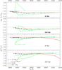 |
Fig. 7 Lithium and iron surface abundance isochrones at 12 Gyr and 13.5 Gyr for models with and without mass loss as well as the T6.09 models with turbulence but no mass loss. The straight line segments link models (dots) calculated with the same physics. The horizontal dotted line at A(7Li) = 2.27 indicates the initial lithium abundance for all models. The model masses are not the same for every isochrone. |
Figure 7 shows lithium and iron isochrones for the diffusion only model, for models with mass loss rates of 10-12 M⊙ yr-1 and 5 × 10-13 M⊙ yr-1, as well as for T6.09 models9 at 12 Gyr and 13.5 Gyr. To simplify the discussion only the effect of mass loss is considered in this section. The T6.09 isochrones that are from Richard et al. (2002b) are discussed in Sect. 5 and where the effects of mass loss and turbulence are compared and the meaning of T6.09 is briefly described.
In the diffusion only model, large Fe and Li anomalies are obtained around turnoff: lithium decreases by a factor of up to 10 at 12 Gyr, while Fe becomes overabundant by a factor of 5. For the mass loss rate of 5 × 10-13 M⊙ yr-1, the maximum lithium underabundance is reduced to −0.35 dex, whereas Fe overabundances are transformed into underabundances by factors below −0.25 dex. For the 10-12 M⊙ yr-1 model, the maximum amplitudes are further reduced. While the anomalies in the diffusion only model near turnoff are much smaller at 13.5 Gyr than at 12 Gyr, this effect is not as important for lithium, and is unnoticeable for both models with mass loss.
Below ~6000 K, the lithium isochrones with and without mass loss differ only slightly for preturnoff stars – with lithium depletions between − 0.12 and − 0.14 dex near Teff = 5400 K – since the SCZ is too deep for mass loss to have an effect. Though all three isochrones have decreasing lithium abundances for models hotter than ~6000 K, the underabundance amplitude decreases as the mass loss rate increases. At 12 Gyr, the lithium abundance begins increasing again near 6200 K and 6400 K for the models with 10-12 M⊙ yr-1 and 5 × 10-13 M⊙ yr-1 respectively. This is due to SCZ retraction, which exposes layers for which vwind is dominant.
The diffusion only lithium isochrones do not exhibit plateau-like behavior. On the other hand, the mass loss isochrones are much flatter: the 5 × 10-13 M⊙ yr-1 model has a scatter of about ~0.1 dex and the 10-12 M⊙ yr-1 model has a scatter of about ~0.05 dex with respective plateau average values of about −0.3 dex and −0.2 dex below the initial 7Li abundance.
4. Comparison to previous calculations with mass loss
 |
Fig. 8 (Left panel) Internal lithium profiles for 0.75 M⊙ models with and without mass loss. Three models of different masses were added (colored curves) in order to verify the solution for the 0.75W1E-12 model. (Right panel) A comparison of diffusion (dotted and solid lines) and wind velocities (dashed lines identified in the figure) for the 0.75 M⊙ models. The vertical solid line identifies the bottom of the surface convection zone. All models are shown at 10 Gyr. The left panel can be compared to Fig. 4 of Vauclair & Charbonnel (1995). |
In previous evolutionary calculations for Population II stars with mass loss, Vauclair & Charbonnel (1995, VC95) found that both mass loss rates of 10-12.5 (≃3 × 10-13) and 10-12 M⊙ yr-1 lead to lithium abundances that increase monotonously (by at most 0.5 dex for the lower mass loss rate) with Teff for six models ranging from 0.60 to 0.80 M⊙. They suggested that the higher mass loss rate completely wipes out the effects of atomic diffusion, and leads to a primordial lithium abundance of A(Li) = 2.5 ± 0.1, which they determined from the surface abundance of their hottest model.
Unfortunately, a detailed comparison to their results is impossible, since, even without mass loss, the stellar models are too different. These differences include Y0, Z0, αMLT, the surface boundary condition, and the diffusion of metals. As a result, the SCZ evolution is very different. For instance, by comparing the internal lithium profile of the diffusion only model in Fig. 8 with the one from Fig. 4 of Vauclair & Charbonnel (1995), one sees that at 10 Gyr, the SCZ (i.e. the flat part of the profile for both solutions) is about four times more massive in their models. Furthermore, their 0.75 M⊙ models are still on the MS (with their Teff still increasing) at 18 Gyr, while our 0.75 M⊙ models have already evolved toward the subgiant branch at 15 Gyr. The difference in Y0 is not large enough to explain this significant discrepancy10.
That being said, some general results can still be compared. For instance, at 10 Gyr, VC95 found that the surface lithium abundance for the 10-12.5 M⊙ yr-1 model was 0.12 dex larger than in the 10-12 M⊙ yr-1 model, since the stronger mass loss rate reaches into the lithium burning layers. Our models also suggest that the strongest wind drags some material from the lithium depleted layers outward. Indeed, from Fig. 8, the wind velocity for the 10-12 M⊙ yr-1 model at 10 Gyr dominates the settling velocity down to log ΔM/M∗ = −1, the point of separation, which is well into the burning layers. However, at 10 Gyr, this has not yet reached the surface since at 1010 yr, a mass loss rate of 10-12 M⊙ yr-1 has only exposed to the surface layers which are above ~10-2 M∗. In the same way, mass loss advected all mass above the point of separation, thus explaining the difference in the depths at which Li falls to zero in the diffusion only and 10-12 M⊙ yr-1 models.
Furthermore, the shape of the internal solutions in both sets of models is very different; for 10-12 M⊙ yr-1, VC95 obtain a nearly flat solution from the BSCZ down to Li–burning layers (see their Fig. 4), whereas our solution suggests an important atomic diffusion–induced gradient below the SCZ (see Fig. 8). In order to verify that the difference was not simply due to differences between SCZ masses during evolution, this result was compared to smaller mass models with the same mass loss rate (the 0.73W1E-12, 0.70W1E-12 and 0.68W1E-12 models). Even in models with more massive SCZs, the abundance gradient remains, since it is formed below log ΔM/M∗ ~ − 2, the point above which the wind has imposed the conservation of flux. The reason for these differences between the two calculations is not evident.
The Li profiles in the left panel of Fig. 8 are understood using the right panel and the assumption of unseparated mass loss from the surface. In the 0.75 M⊙ diffusion only model, the gradient between log ΔM/M∗ = −1.8 and –2.7 is determined mainly by the increasing settling time scale as log ΔM/M∗ increases, that is closer to stellar center. In the 0.75W1E-13 model the wind only shifts 10-3 of a solar mass in 1010 years which only very slightly modifies the profile around log ΔM/M∗ ~ −2. In the 0.75W1E-12.5 model the effect is slightly more pronounced as the mass loss velocity becomes a little larger, in magnitude, than the diffusion velocity as seen in the right panel. In the 0.75W1E-12 model however the mass loss velocity is larger than the diffusion velocity by a factor of up to six, and flux conservation determines the Li abundance between log ΔM/M∗ = −1.8 and − 2.7 as discussed in detail in Sect. 5.1.1 of Vick et al. (2010). Since the mass loss from the surface in unseparated and the outgoing Li concentration is the Li concentration in the convection zone, this implies no separation in the convection zone and the Li mass loss flux is X(Li)ρvwind. It is as if the diffusion velocity were zero there. Below the convection zone the Li flux is ~X(Li)ρ(vwind − vD). Element conservation at the BSCZ forces a strong gradient just below11. It is seen mainly in the 0.75W1E-12 and 0.73W1E-12 models. Because the wind velocity hardly exceeds the diffusion velocity below the bottom of the SCZ in the 0.68 M⊙ model, the gradient is less abrupt in that model.
 |
Fig. 9 Evolution of the surface abundances of Li, Fe, and Ca as a function of Teff for two models with turbulence and two with mass loss identified in the figure. The chosen scale emphasizes the behavior on the subgiant and bottom of the giant branch. All models start (pre-main-sequence) to the right of the upper horizontal line and evolve to the left until they reach the main sequence at Teff ~ 6100 K. Then, diffusion starts being effective and the Li abundance, for instance, is reduced by 0.2 to 0.4 dex as the star approaches turnoff, at Teff ~ 6600 K. The models then move to the subgiant and giant branches where dilution further reduces the surface Li abundance by a factor of ~10. For Ca and Fe the radiative acceleration complicates the surface abundance evolution in the mass loss cases. |
Finally, while VC95 obtain no effects of chemical separation in all models with 10-12 M⊙ yr-1 (see the caption of their Fig. 4), lithium settling leads to ~0.15 dex surface abundance reductions (at 12 Gyr) in all our models (see Fig. 7). In terms of isochrone shape, VC95 obtain a monotonous linear increase from the cooler stars to the hotter ones (Figs. 5 and 6 of VC95), while our isochrones dip in the interval 6400 K ≥ Teff ≥ 6000 K (Fig. 7).
Some of the differences are related to the difference in models, namely the ΔMBSCZ evolution. Other differences could include the way the boundary condition below the SCZ was written and the fact that the wind term in their diffusion equation does not include the often overlooked flux factor (mr/M∗) which is required in evolutionary models (see Eq. (6) of Paper I). This factor changes vwind by 1% at log ΔM/M∗ = −2 and by 10% at log ΔM/M∗ = −1. Given that wind and diffusion velocities are comparable for many elements near log ΔM/M∗ = −1 (see Figs. 3 and 4), this term modifies central concentrations. For instance, in the 0.779 M⊙ model with a mass loss rate of 5 × 10-13 M⊙ yr-1, the central hydrogen concentration decreases below 10-3, ~1.3 Gyr earlier when the correction term is included. The effect on surface concentrations is, however, very small.
5. Comparison to models with turbulence
Along with describing the effects of mass loss on Population II evolutionary models with mass loss, this paper’s main objective is to contrast models with mass loss to the ones with turbulence presented in Richard et al. (2002b). In particular, one goal is to see if a specific mass loss rate can reproduce the surface abundances exhibited in the T6.09 models9 around turnoff, which are compatible with the Spite plateau (Richard et al. 2005).
In Fig. 6, the surface abundances of the 0.80T6.09 and 0.80W1E-12 models are shown to be very similar. Abundances of 4He and 7Li are about 0.02 dex smaller in the model with turbulence, whereas elements with Z > 12 are on average about 0.03–0.04 dex smaller (with a maximum of about 0.05 dex for Ar). The differences in surface abundances of elements from Be to Mg are smaller than the line width.
In terms of lithium and iron isochrones, as shown in Fig. 7, the differences are just as small. Both types of models lead to nearly flat abundances (above Teff = 5800 K), and their plateau value is nearly the same. At 12 Gyr, the maximum difference in Fe abundance, which occurs near Teff ≃ 6100 K, is about 0.07 dex, though this could be due to the absence of turbulent models in this region. Similarly, for models hotter than Teff = 5800 K, the maximum difference in 7Li abundances, which occurs at Teff ≃ 6200 K, is 0.1 dex, and could again be explained by the T6.09 isochrone’s poor resolution. Below Teff = 5800 K, larger differences appear for lithium, likely due to lithium destruction in the model with turbulence. The discrepancy is greater than 0.3 dex, although again, the resolution is not sufficient to quantify precisely the difference.
Whereas the surface behavior is quite similar for most models with T6.09 and 10-12 M⊙ yr-1, the internal solutions are a little more different. By comparing Fig. 3 with Fig. 8 of Richard et al. (2002b), one notes that in the 0.80W1E-12 model, abundances change gradually from the bottom of the SCZ down to about log ΔM/M∗ = −1, with most variations between 0.1 and 0.15 dex. However, in the 0.80T6.09 model at turnoff, abundances are constant from the surface down to just below log ΔM/M∗ = −2. Even though in the mass loss models the abundance variations are relatively small, and the corresponding changes in opacity are likely to be small as well, this could potentially be tested by asteroseismic observations.
6. Subgiant and giant branches
The evolution of the surface abundances of Li, Fe, and Ca are shown in Fig. 9 for 0.779 M⊙ models with Z0 = 0.0002712. It is shown as a function of Teff in order to facilitate comparison with stars on the subgiant and giant branches. At turnoff, the T6.25 model has approximately the same Li abundance as the 5 × 10-13 M⊙ yr-1 model and the T6.09 model approximately the same as the 10-12 M⊙ yr-1 model. Past turnoff, the surface Li abundance first increases in both models with mass loss (with a maximum at Teff ~ 5800 K) as the peak in Li abundance seen at log ΔM/M∗ ~ −2 in the left panel of Fig. 8 is mixed to the surface. In the models with turbulence, this Li peak is either reduced (T6.09 model) or eliminated (T6.25 model) as may be seen in Fig. 7 of Richard et al. (2005). In the latter model, the Li abundance decreases continuously past turnoff to ~−1.5 on the giant branch (Teff < 5000 K). More Li has been destroyed by turbulence in the T6.25 model than carried away by a mass loss rate of 10-12 M⊙ yr-1 since the Li abundance on the giant branch is smaller in the T6.25 model than in the mass loss one. This implies that turbulence leads to a 0.2 dex additional destruction of Li in the T6.25 model when compared to models with atomic diffusion alone.
These results may be compared to the calculations and observations of Mucciarelli et al. (2011) and of Nordlander et al. (2012). The T6.25 model leads to an additional 0.2 dex destruction of Li as appears required for the observations of Li in lower red giant branch stars (Mucciarelli et al. 2011) to be compatible with WMAP measurements. Neither of the mass loss models leads to as large a reduction of surface Li on the giant branch as the T6.25 model, so that the RGB observations favor the turbulent T6.25 model. However, one may also compare our results to the Li observations in Figs. 2 and 5 of Nordlander et al. (2012) where isochrones of Li abundance are compared to observations of NGC 6397. While we do not have isochrones, a comparison is possible using evolutionary variations of Li abundance since the same turbulent models were used in our calculations and for their Figs. 2 and 5. If one compares the 10-12 M⊙ yr-1 results, to the T6.0 preferred by Nordlander et al. (2012), one notes similar agreement at turnoff, but better agreement on the subgiant branch since maxima in our Fig. 9 appear at a slightly higher Teff and are more pronounced for the 10-12 M⊙ yr-1 model than for the two turbulent cases. The agreement is also better for the bRGB and RGB observations since the 10-12 M⊙ yr-1 curve is lower than even the T6.09 curve in our Fig. 9. It then appears that models with mass loss lead to at least as good agreement with Li observations as do models with turbulence.
For Ca and Fe, the radiative accelerations complicate the evolution in the mass loss cases. For instance, the large Ca abundance close to the surface for the 11.664 Gyr curve for Ca on Fig. 3 is caused by the grad(Ca) minimum as discussed in relation to that figure. In turn it appears as the abundance maximum at Teff ~ 6500 K in Fig. 9. The Fe local maximum at Teff ~ 6000 K in Fig. 9 is similarly caused by the grad(Fe) minimum for the 11.664 Gyr curve at log ΔM/M∗ ~ −3 in Fig. 3. These properties affect the comparison to observations for the mass loss models. The comparison is shown for the turbulent models in Fig. 2 of Nordlander et al. (2012). If one assumes the abundance shifts just discussed, the agreement with observations would be poorer with the mass loss models for both Fe and Ca at Teff ~ 6400 K while at Teff ~ 6000 K, it would be poorer for Fe and unchanged for Ca.
Given the difficulty justifying such a high mass loss rate we did not push the comparison with observations further.
7. Conclusion
Evolutionary models with atomic diffusion and unseparated mass loss explain some characteristics observed in galactic halo dwarfs. A mass loss rate of 5 × 10-13 M⊙ yr-1 leads to surface lithium isochrones that exhibit plateau-like behavior with a maximum scatter of about 0.1 dex around an average value that is − 0.3 dex below the initial lithium abundance (Fig. 7). For models with mass loss rates of 10-12 M⊙ yr-1, the lithium isochrones are even flatter with a scatter of about 0.05 dex around an average value about − 0.2 dex lower than the initial abundance.
While mass loss does not have a significant impact on a star’s structural properties, its effects on abundances, both in the interior and on the surface, can be important. In the interior, abundance profiles are either dominated by atomic diffusion – and reflect local variations in grad – or are dominated by the wind – and adjust in order to conserve the flux coming from below (Sect. 3.1). A mass loss rate of 10-13 M⊙ yr-1 reduces both internal and surface anomalies by up to a factor of 6–7, while a mass loss rate of 10-12 M⊙ yr-1 reduces all anomalies to below 0.2 dex (Fig. 4 and 6). While the 10-12 M⊙ yr-1 models lead to generalized underabundances for all elements, lower mass loss rates allow for overabundances to develop at the surface.
The mass loss models presented in this paper differ significantly from those presented in Vauclair & Charbonnel (1995) (Fig. 8). Although some of this difference can be attributed to differences in input parameters, other discrepancies are more difficult to explain (Sect. 4). In one critical aspect however, the results are robust: both calculations conclude that below 10-14 M⊙ yr-1 mass loss has virtually no effect while above 10-12 M⊙ yr-1 it eliminates all effects of atomic diffusion from the surface.
With respect to the T6.09 models from Richard et al. (2002b), the models with a mass loss rate of 10-12 M⊙ yr-1 are very similar above Teff = 5800 K (Figs. 6 and 7). Below this temperature, turbulence leads to greater lithium destruction. Because of differences in the internal distribution of elements (Sect. 5), asteroseismology could perhaps distinguish between the two scenarios.
Unfortunately, even for mass loss rates of 10-12 M⊙ yr-1, the implied stellar winds are barely detectable through direct observation. Furthermore, considering that acceleration processes for these types of winds are unknown, it is difficult to justify mass loss rates that are 50 times higher than the solar mass loss rate (~2 × 10-14 M⊙ yr-1). It is unlikely that winds in Population II stars are driven by radiation; therefore, if these stars host solar-like winds, one could hope to observe solar-like coronae and/or X-ray emission.
A signature of a chromosphere has recently been observed in Pop II dwarfs: the He line 10 830 A is present in almost all dwarfs with [Fe/H] = −0.5 to −3.7 (Takeda & Takada-Hidai 2011). Signs of chromospheres had earlier been reported in these stars by Peterson & Schrijver (2001). On the other hand, Cranmer & Saar (2011) have recently evaluated mass loss rates in various types of stars. According to their Fig. 13, mass loss rates of ~10-12 M⊙ yr-1 are to be expected in dwarf stars of Teff ~ 6000 K of solar metallicity that have rotation periods of around six days. They do not give equivalent values for lower metallicity stars. The most critical factor is, however, the rotation rate. Pop II dwarfs are believed to rotate slowly. However, there are observations (reviewed in Fig. 6 of Takeda & Takada-Hidai 2011) suggesting that many rotate at vesini ~ 5 km s-1. It would seem important to confirm both the rotation rate observations and expected mass loss rates for low metallicity stars. In the meantime it seems premature to disregard mass loss as a process competing with atomic diffusion in Pop II stars.
As a next step, these models could be extended to the He flash in order to further constrain the effects of mass loss in Population II giants, for which mass loss has extensively been observed and studied (Origlia et al. 2007). It would also be interesting to see if such mass loss rates would affect, or even eliminate, the effects of atomic diffusion (Michaud et al. 2010) and/or of thermohaline mixing (Charbonnel & Zahn 2007; Traxler et al. 2011).
Online material
Appendix A: Version of Figs. 3 and 4 with all atomic species included in the calculations
 |
Fig. A.1 Radiative accelerations and gravity at four different ages in a 0.8 M⊙ model with Ṁ = 10-12 M⊙ yr-1. The vertical lines indicate the position of the bottom of the SCZ. The ages are identified in the figure. |
 |
Fig. A.2 Abundance profiles at four different ages in a 0.8 M⊙ model with Ṁ = 10-12 M⊙ yr-1 and an initial metallicty of Z0 = 0.00017. The vertical lines indicate the position of the bottom of the SCZ. The ages are identified in the figure. |
 |
Fig. A.3 Abundance profiles for the model without mass loss and for mass loss rates, from Ṁ = 10-14 M⊙ yr-1 to Ṁ = 10-12 M⊙ yr-1 in a 0.8 M⊙ model and an initial metallicty of Z0 = 0.00017. The internal concentration profiles are shown just before turnoff near 11.5 Gyr. The vertical lines indicate the position of the bottom of the SCZ. The mass loss rates are identified in the figure. |
 |
Fig. A.4 Evolution of surface abundances for the model without mass loss (dotted line) and for mass loss rates, from Ṁ = 10-15 M⊙ yr-1, to Ṁ = 10-12 M⊙ yr-1 in a 0.8 M⊙ model and an initial metallicty of Z0 = 0.00017. One cannot distinguish the curves for the model without mass loss from those for the model with Ṁ = 10-15 M⊙ yr-1. The mass loss rates are identified in the figure. |
From the Wilkinson Microwave Anisotropic Background (WMAP), see Spergel et al. (2007).
A(Li) = log [N(Li)/N(H) + 12].
In this context, unseparated refers to the abundances in the wind being the same as in the photosphere.
0.80W1E-12 refers to a 0.80 M⊙ model with a mass loss rate of 1 × 10-12 M⊙ yr-1.
This mass was chosen to facilitate comparison with the models and figures from Richard et al. (2002b).
The mass loss rate also has little to no effect on grad for this same reason, and because its effects on the structure are very small (see Fig. 2).
To be more precise, in the stellar core, these elements arrive at an equilibrium between multiple ionization states, including the hydrogenic one.
We have verified that the 10-15 M⊙ yr-1 model is the same as the no-mass-loss model. See Fig. 2.
The parameters specifying turbulent transport coefficients are indicated in the name assigned to the model. For instance, in the T6.09D400-3 model, the turbulent diffusion coefficient, DT, is 400 times greater than the He atomic diffusion coefficient at log T0 = 6.09 and varying as ρ-3, or
![Mathematical equation: \begin{equation} \label{eq:DTT} \Dturb=400 D_{\mathrm{He}}(T_0)\left[\frac{\rho}{\rho(T_0)}\right]^{-3}\cdot \end{equation}](/articles/aa/full_html/2013/04/aa20726-12/aa20726-12-eq76.png) (1)
To simplify writing, T6.09 is also used instead of T6.09D400-3 since all models discussed in this paper have the D400-3 parametrization. The 0.80T6.09 model is a 0.80 M⊙ model with T6.09 turbulence.
(1)
To simplify writing, T6.09 is also used instead of T6.09D400-3 since all models discussed in this paper have the D400-3 parametrization. The 0.80T6.09 model is a 0.80 M⊙ model with T6.09 turbulence.
Though not shown, this was verified by evolving models with Y0 = 0.2484, whose lower H mass fraction in the core led to their passing turnoff only 1 Gyr earlier than models with Y0 = 0.2352. The models from Vauclair & Charbonnel (1995) have Y0 = 0.2403.
More technically, the diffusion term in vD must compensate for the decrease in X(Li) as one approaches the convection zone. Except where there is a strong X(Li) gradient, only the advective part of vD plays a significant role. Numerical accuracy required some one hundred zones in the small region of the strong gradient.
Acknowledgments
M. Vick would like to thank the Département de physique de l’Université de Montréal for financial support, along with everyone at the GRAAL in Montpellier for their amazing hospitality. We acknowledge the financial support of Programme National de Physique Stellaire (PNPS) of CNRS/INSU, France. This research was partially supported by NSERC at the Université de Montréal. Finally, we thank Calcul Québec for providing us with the computational resources required for this work. We thank an anonymous referee for useful comments.
References
- Aoki, W., Barklem, P. S., Beers, T. C., et al. 2009, ApJ, 698, 1803 [NASA ADS] [CrossRef] [Google Scholar]
- Asplund, M., Lambert, D. L., Nissen, P. E., Primas, F., & Smith, V. V. 2006, ApJ, 644, 229 [NASA ADS] [CrossRef] [Google Scholar]
- Böhm-Vitense, E. 1992, Introduction to Stellar Astrophysics (Cambridge, UK: Cambridge University Press), 3 [Google Scholar]
- Bonifacio, P. 2002, A&A, 395, 515 [NASA ADS] [CrossRef] [EDP Sciences] [Google Scholar]
- Bonifacio, P., Molaro, P., Sivarani, T., et al. 2007, A&A, 462, 851 [NASA ADS] [CrossRef] [EDP Sciences] [Google Scholar]
- Cayrel, R., Steffen, M., Chand, H., et al. 2007, A&A, 473, L37 [NASA ADS] [CrossRef] [EDP Sciences] [Google Scholar]
- Charbonnel, C., & Primas, F. 2005, A&A, 442, 961 [NASA ADS] [CrossRef] [EDP Sciences] [Google Scholar]
- Charbonnel, C., & Talon, S. 2005, Science, 309, 2189 [NASA ADS] [CrossRef] [PubMed] [Google Scholar]
- Charbonnel, C., & Zahn, J. 2007, A&A, 467, L15 [NASA ADS] [CrossRef] [EDP Sciences] [Google Scholar]
- Charbonnel, C., Vauclair, S., & Zahn, J. 1992, A&A, 255, 191 [NASA ADS] [Google Scholar]
- Coc, A., Vangioni-Flam, E., Descouvemont, P., Adahchour, A., & Angulo, C. 2004, ApJ, 600, 544 [NASA ADS] [CrossRef] [Google Scholar]
- Cranmer, S. R., & Saar, S. H. 2011, ApJ, 741, 54 [NASA ADS] [CrossRef] [Google Scholar]
- Cumberbatch, D., Ichikawa, K., Kawasaki, M., et al. 2007, Phys. Rev. D, 76, 123005 [NASA ADS] [CrossRef] [Google Scholar]
- Cyburt, R. H., Fields, B. D., & Olive, K. A. 2003, Phys. Lett. B, 567, 227 [NASA ADS] [CrossRef] [Google Scholar]
- Cyburt, R. H., Fields, B. D., & Olive, K. A. 2008, J. Cosmol. Astro-Part. Phys., 11, 12 [Google Scholar]
- Deliyannis, C. P., Demarque, P., & Kawaler, S. D. 1990, ApJS, 73, 21 [NASA ADS] [CrossRef] [Google Scholar]
- Gonzalez, J.-F., LeBlanc, F., Artru, M.-C., & Michaud, G. 1995, ApJ, 297, 223 [Google Scholar]
- González Hernández, J. I., Bonifacio, P., Caffau, E., et al. 2009, A&A, 505, L13 [NASA ADS] [CrossRef] [EDP Sciences] [Google Scholar]
- Ichikawa, K., Kawasaki, M., & Takahashi, F. 2004, Phys. Lett. B, 597, 1 [NASA ADS] [CrossRef] [Google Scholar]
- Iglesias, C. A., & Rogers, F. 1996, ApJ, 464, 943 [NASA ADS] [CrossRef] [Google Scholar]
- Korn, A. J., Grundahl, F., Richard, O., et al. 2006, Nat, 442, 657 [NASA ADS] [CrossRef] [Google Scholar]
- Korn, A. J., Grundahl, F., Richard, O., et al. 2007, ApJ, 671, 402 [NASA ADS] [CrossRef] [Google Scholar]
- Krishna-Swamy, K. S. 1966, ApJ, 145, 176 [Google Scholar]
- LeBlanc, F., Michaud, G., & Richer, J. 2000, ApJ, 538, 876 [NASA ADS] [CrossRef] [Google Scholar]
- Lind, K., Primas, F., Charbonnel, C., Grundahl, F., & Asplund, M. 2009, A&A, 503, 545 [NASA ADS] [CrossRef] [EDP Sciences] [MathSciNet] [Google Scholar]
- Lind, K., Asplund, M., Collet, R., & Meléndez, J. 2012, Mem. Soc. Astron. It. Supp., 22, 142 [Google Scholar]
- Meléndez, J., & Ramírez, I. 2004, ApJ, 615, L33 [NASA ADS] [CrossRef] [Google Scholar]
- Meléndez, J., Casagrande, L., Ramírez, I., Asplund, M., & Schuster, W. J. 2010, A&A, 515, L3 [NASA ADS] [CrossRef] [EDP Sciences] [Google Scholar]
- Michaud, G., Fontaine, G., & Beaudet, G. 1984, ApJ, 282, 206 [NASA ADS] [CrossRef] [Google Scholar]
- Michaud, G., Richer, J., & Richard, O. 2007, ApJ, 670, 1178 [NASA ADS] [CrossRef] [Google Scholar]
- Michaud, G., Richer, J., & Richard, O. 2008, ApJ, 675, 1223 [NASA ADS] [CrossRef] [Google Scholar]
- Michaud, G., Richer, J., & Richard, O. 2010, A&A, 510, A104 [NASA ADS] [CrossRef] [EDP Sciences] [Google Scholar]
- Michaud, G., Richer, J., & Vick, M. 2011, A&A, 534, A18 [NASA ADS] [CrossRef] [EDP Sciences] [Google Scholar]
- Mucciarelli, A., Salaris, M., Lovisi, L., et al. 2011, MNRAS, 412, 81 [NASA ADS] [CrossRef] [Google Scholar]
- Nordlander, T., Korn, A. J., Richard, O., & Lind, K. 2012, ApJ, 753, 48 [NASA ADS] [CrossRef] [Google Scholar]
- Origlia, L., Rood, R. T., Fabbri, S., et al. 2007, ApJ, 667, L85 [NASA ADS] [CrossRef] [Google Scholar]
- Peterson, R. C. & Schrijver, C. J. 2001, in 11th Cambridge Workshop on Cool Stars, Stellar Systems and the Sun, eds. R. J. Garcia Lopez, R. Rebolo, & M. R. Zapaterio Osorio, ASP Conf. Ser., 223, 300 [Google Scholar]
- Piau, L., Beers, T. C., Balsara, D. S., et al. 2006, ApJ, 653, 300 [NASA ADS] [CrossRef] [Google Scholar]
- Pinsonneault, M. H., Walker, T. P., Steigman, G., & Narayanan, V. K. 1999, ApJ, 527, 180 [NASA ADS] [CrossRef] [Google Scholar]
- Profitt, C. R., & Michaud, G. 1991, ApJ, 371, 584 [NASA ADS] [CrossRef] [Google Scholar]
- Regis, M., & Clarkson, C. 2012, Gen. Relativ. Grav., 44, 567 [Google Scholar]
- Richard, O., Michaud, G., & Richer, J. 2001, ApJ, 558, 377 [NASA ADS] [CrossRef] [Google Scholar]
- Richard, O., Michaud, G., & Richer, J. 2002a, ApJ, 580, 1100 [NASA ADS] [CrossRef] [Google Scholar]
- Richard, O., Michaud, G., Richer, J., et al. 2002b, ApJ, 568, 979 [Google Scholar]
- Richard, O., Michaud, G., & Richer, J. 2005, ApJ, 619, 538 [NASA ADS] [CrossRef] [Google Scholar]
- Richer, J., Michaud, G., Rogers, F., Turcotte, S., & Iglesias, C. A. 1998, ApJ, 492, 833 [NASA ADS] [CrossRef] [Google Scholar]
- Richer, J., Michaud, G., & Turcotte, S. 2000, ApJ, 529, 338 [NASA ADS] [CrossRef] [Google Scholar]
- Ryan, S. G., Norris, J. E., & Beers, T. C. 1999, ApJ, 523, 654 [NASA ADS] [CrossRef] [Google Scholar]
- Salaris, M., Groenewegen, M. A. T., & Weiss, A. 2000, A&A, 355, 299 [NASA ADS] [Google Scholar]
- Sbordone, L., Bonifacio, P., Caffau, E., et al. 2010, A&A, 522, A26 [NASA ADS] [CrossRef] [EDP Sciences] [Google Scholar]
- Sbordone, L., Bonifacio, P., & Caffau, E. 2012, Mem. Soc. Astron. It. Supp., 22, 29 [Google Scholar]
- Spergel, D. N., Bean, R., Doré, O., et al. 2007, ApJS, 170, 377 [NASA ADS] [CrossRef] [Google Scholar]
- Spite, F., & Spite, M. 1982, A&A, 115, 357 [NASA ADS] [Google Scholar]
- Spite, M., Spite, F., & Maillard, J. P. 1984, A&A, 141, 56 [NASA ADS] [Google Scholar]
- Steigman, G. 2007, Ann. Rev. Nucl. Part. Sci., 57, 463 [Google Scholar]
- Takeda, Y., & Takada-Hidai, M. 2011, PASJ, 63, 547 [NASA ADS] [Google Scholar]
- Talon, S., & Charbonnel, C. 2004, A&A, 418, 1051 [NASA ADS] [CrossRef] [EDP Sciences] [Google Scholar]
- Traxler, A., Garaud, P., & Stellmach, S. 2011, ApJ, 728, L29 [NASA ADS] [CrossRef] [Google Scholar]
- Turcotte, S., Richer, J., Michaud, G., Iglesias, C. A., & Rogers, F. 1998, ApJ, 504, 539 [NASA ADS] [CrossRef] [Google Scholar]
- VandenBerg, D. A., Bolte, M., & Stetsson, P. B. 1996, ARA&A, 34, 461 [NASA ADS] [CrossRef] [Google Scholar]
- VandenBerg, D. A., Swenson, F. J., Rogers, F. J., Iglesias, C. A., & Alexander, D. R. 2000, ApJ, 532, 430 [NASA ADS] [CrossRef] [Google Scholar]
- VandenBerg, D. A., Richard, O., Michaud, G., & Richer, J. 2002, ApJ, 571, 487 [NASA ADS] [CrossRef] [EDP Sciences] [Google Scholar]
- VandenBerg, D. A., Edvardsson, B., Eriksson, K., & Gustafsson, B. 2008, ApJ, 675, 746 [NASA ADS] [CrossRef] [Google Scholar]
- Vauclair, S. 1988, ApJ, 335, 971 [NASA ADS] [CrossRef] [Google Scholar]
- Vauclair, S., & Charbonnel, C. 1995, A&A, 295, 715 [NASA ADS] [Google Scholar]
- Vick, M., Michaud, G., Richer, J., & Richard, O. 2010, A&A, 521, A62 [NASA ADS] [CrossRef] [EDP Sciences] [Google Scholar]
- Vick, M., Michaud, G., Richer, J., & Richard, O. 2011, A&A, 526, A37 [NASA ADS] [CrossRef] [EDP Sciences] [Google Scholar]
All Figures
|
Fig. 1 The Hertzprung-Russel diagram, as well as the evolution of Teff, log g, the temperature at the base of the SCZ (TBSCZ), the outer mass at the base of the SCZ (ΔMBSCZ), and the mass fraction of hydrogen in the core (Xc) for stars of 0.6 − 0.8 M⊙ with Z0 = 0.00017 and Ṁ = 10-12 M⊙ yr-1. |
| In the text | |
|
Fig. 2 The impact of mass loss on the evolution of the depth (in temperature and mass) of the SCZ in 0.8 M⊙ models with atomic diffusion only, and with mass loss rates from 10-15 M⊙ yr-1 to 10-12 M⊙ yr-1. Upper row: HR diagram and the He and Fe surface abundances. Lower row: zoom on the Teff, and on the mass and temperature at the bottom of the SCZ. |
| In the text | |
|
Fig. 3 Upper row: radiative accelerations (solid lines) and gravity (dotted lines); center row: wind velocities (dashed lines) and diffusion velocities toward the exterior (solid lines) and toward the interior (dotted lines); lower row: interior concentrations as a fraction of original ones. These quantities are shown at four different ages for a 0.8 M⊙ model with Ṁ = 10-12 M⊙ yr-1. The vertical lines indicate the position of the bottom of the SCZ. The ages are identified in the figure. |
| In the text | |
|
Fig. 4 The impact of mass loss rate on internal abundance profiles for 0.80 M⊙ models. A model without mass loss and models with five mass loss rates from 10-14 M⊙ yr-1 to 10-12 M⊙ yr-1 are shown and are identified in the figure. The internal concentration profiles are shown just before turnoff near 11.5 Gyr. Atomic diffusion affects mainly the outer 10-2 of the stellar mass. Conventions are similar to those of Fig. 3. |
| In the text | |
|
Fig. 5 Evolution of surface abundance anomalies for selected stellar masses and elements with a mass loss rate of 10-12 M⊙ yr-1. |
| In the text | |
|
Fig. 6 Surface abundance anomalies for 0.8 M⊙ models with and without mass loss as well as with the T6.09 turbulent parametrization. At 11.5 Gyr, these models are just before turnoff. |
| In the text | |
|
Fig. 7 Lithium and iron surface abundance isochrones at 12 Gyr and 13.5 Gyr for models with and without mass loss as well as the T6.09 models with turbulence but no mass loss. The straight line segments link models (dots) calculated with the same physics. The horizontal dotted line at A(7Li) = 2.27 indicates the initial lithium abundance for all models. The model masses are not the same for every isochrone. |
| In the text | |
|
Fig. 8 (Left panel) Internal lithium profiles for 0.75 M⊙ models with and without mass loss. Three models of different masses were added (colored curves) in order to verify the solution for the 0.75W1E-12 model. (Right panel) A comparison of diffusion (dotted and solid lines) and wind velocities (dashed lines identified in the figure) for the 0.75 M⊙ models. The vertical solid line identifies the bottom of the surface convection zone. All models are shown at 10 Gyr. The left panel can be compared to Fig. 4 of Vauclair & Charbonnel (1995). |
| In the text | |
|
Fig. 9 Evolution of the surface abundances of Li, Fe, and Ca as a function of Teff for two models with turbulence and two with mass loss identified in the figure. The chosen scale emphasizes the behavior on the subgiant and bottom of the giant branch. All models start (pre-main-sequence) to the right of the upper horizontal line and evolve to the left until they reach the main sequence at Teff ~ 6100 K. Then, diffusion starts being effective and the Li abundance, for instance, is reduced by 0.2 to 0.4 dex as the star approaches turnoff, at Teff ~ 6600 K. The models then move to the subgiant and giant branches where dilution further reduces the surface Li abundance by a factor of ~10. For Ca and Fe the radiative acceleration complicates the surface abundance evolution in the mass loss cases. |
| In the text | |
|
Fig. A.1 Radiative accelerations and gravity at four different ages in a 0.8 M⊙ model with Ṁ = 10-12 M⊙ yr-1. The vertical lines indicate the position of the bottom of the SCZ. The ages are identified in the figure. |
| In the text | |
|
Fig. A.2 Abundance profiles at four different ages in a 0.8 M⊙ model with Ṁ = 10-12 M⊙ yr-1 and an initial metallicty of Z0 = 0.00017. The vertical lines indicate the position of the bottom of the SCZ. The ages are identified in the figure. |
| In the text | |
|
Fig. A.3 Abundance profiles for the model without mass loss and for mass loss rates, from Ṁ = 10-14 M⊙ yr-1 to Ṁ = 10-12 M⊙ yr-1 in a 0.8 M⊙ model and an initial metallicty of Z0 = 0.00017. The internal concentration profiles are shown just before turnoff near 11.5 Gyr. The vertical lines indicate the position of the bottom of the SCZ. The mass loss rates are identified in the figure. |
| In the text | |
|
Fig. A.4 Evolution of surface abundances for the model without mass loss (dotted line) and for mass loss rates, from Ṁ = 10-15 M⊙ yr-1, to Ṁ = 10-12 M⊙ yr-1 in a 0.8 M⊙ model and an initial metallicty of Z0 = 0.00017. One cannot distinguish the curves for the model without mass loss from those for the model with Ṁ = 10-15 M⊙ yr-1. The mass loss rates are identified in the figure. |
| In the text | |
Current usage metrics show cumulative count of Article Views (full-text article views including HTML views, PDF and ePub downloads, according to the available data) and Abstracts Views on Vision4Press platform.
Data correspond to usage on the plateform after 2015. The current usage metrics is available 48-96 hours after online publication and is updated daily on week days.
Initial download of the metrics may take a while.