| Issue |
A&A
Volume 552, April 2013
|
|
|---|---|---|
| Article Number | A50 | |
| Number of page(s) | 11 | |
| Section | The Sun | |
| DOI | https://doi.org/10.1051/0004-6361/201220427 | |
| Published online | 21 March 2013 | |
Longitudinal magnetic field and velocity gradients in the photosphere inferred from THEMIS multiline observations
LESIA, Observatoire de Paris, CNRS-INSU-UMR 8109, UPMC Univ. Paris 6,
Université Paris Diderot-Paris 7,
5 place Jules Janssen,
92190
Meudon,
France
e-mail:
This email address is being protected from spambots. You need JavaScript enabled to view it.
Received:
21
September
2012
Accepted:
8
February
2013
Abstract
We present multiline observations taken with the French-Italian telescope THEMIS operated by CNRS and CNR on the island of Tenerife. Several spectral lines are observed simultaneously to study magnetic phenomena at different altitudes of line formation, comprising the Fe i 5250.65 Å, Cr i 5247.57 Å, Fe i 5250.22 Å, Fe i 6301.51 Å, Fe i 6302.50 Å, and Fe i 6151.62 Å lines. The observations were analyzed using Milne-Eddington inversion algorithms modified to allow for non-normal Zeeman triplet lines, and to take additionally into account the vertical velocity gradient. We show the self-consistency of the solutions found from the inversion and those obtained from the quantitative bisector method. Results from the different lines observed simultaneously yield the height dependence of the magnetic field strength. From modeling the line formation heights applied on selected points with a longitudinal magnetic field between 200 and 1000 G, we determine the gradient of the vertical component (absolute value) of the magnetic field to be − 1.18 G/km.
Key words: Sun: photosphere / line: profiles / magnetic fields / instrumentation: polarimeters
In memory of our friend and colleague Jean Rayrole.
© ESO, 2013
1. Introduction
Convective motions and atmospheric inhomogeneities leave distinct fingerprints on the spectral lines, which can be used to decipher the conditions produced by convection in the line-forming layers. Line strengths of weak lines are predominantly determined by the average atmospheric temperature structure, while the line widths reflect the amplitude of the Doppler shifts introduced by the velocity fields. Line shifts and bisectors are created by the correlation between temperature and velocity as well as horizontal velocities that might contribute through a geometrical projection effect. Convection plays a dominant role in addition to energy transport mixing of magnetic activity, chromospheric heating, and solar pulsations (Asplund et al. 2000), and leaves distinct signatures in the spectral lines in the form of line asymmetries (Dravins & Nordlund 1990). Bisectors of unblended lines have a characteristic C-shape, which results from the Doppler shifts between up-and downflows. Weak lines normally only show the upper part of the C-shape and have convective blueshift (Asplund et al. 2000). The cores of stronger lines are formed in or above the convective overshoot layers and therefore have a lower or non-existent blueshift (Allende Prieto & Garcia López 1998). Asymmetries in the line profile can be produced by gradients of the velocity along the line of sight, resulting in the familiar C-shape of the line bisector that can be corrected for in the phase measurements by cross-spectral analysis (Grec et al. 2007).
A number of observations have shown that asymmetries in the Stokes V profiles do exist (Grigorjev & Katz 1972, and references therein). Observations of the Stokes V asymmetry in sunspots were first reported by Illing et al. (1974), and were followed by Henson & Kemp (1984) and Makita & Ohki (1986). Observations by Stenflo et al. (1984) and Solanki & Stenflo (1984; 1985) provide evidence of asymmetries in Stokes V profiles in plage regions. Attempts to explain the cause of the asymmetries have been based upon polarized radiative transfer synthesis of Stokes V profiles in the presence of gradients, in both velocity and magnetic fields, using gradients in velocity or magnetic field alone, or atomic orientation (Auer & Heasley 1978; Landman & Finn 1979; Makita 1980; Landi Degl’Innocenti & Landolfi 1982; Ribes et al. 1985; Balasubramaniam et al. 1997; Khomenko et al. 2005). The net circular polarization has been defined as the Stokes V signal integrated over a spectral line. This parameter is null in a perfectly anti-symmetric Stokes V profile, because the area of the blue lobe compensates for the area of the red lobe. The net circular polarization is null if there is no velocity gradient along the line-of-sight. Sanchéz Almeida & Lites (1992) and Landolfi & Landi Degl’Innocenti (1996) showed that a gradient in any of the three components of the magnetic field vector will also enhance the amount of the net circular polarization. Martinez-Pillet (2000) presented observations and properties of the net circular polarization. Müller et al. (2006) showed that the corresponding net circular polarization maps reproduce the general symmetry properties.
More sophisticated methods must be applied, for instance the inversion technique, which allows one to fit the line asymmetry (Khomenko & Collados 2007). A Milne-Eddington inversion assumes that the physical parameters are constant with optical depth and, therefore, it always produces anti-symmetric Stokes V profiles, thereby failing to properly fit the highly asymmetric observed circular polarization signals. We studied the relationship between the C-shape and the Stokes V asymmetries, and explored the possibility that these asymmetric Stokes V profiles imply a strong velocity (and magnetic field) gradient along the line-of-sight (Molodij et al. 2011). We extended the Unno-Rachkovsky solution to provide the theoretical profiles that are derived for a Milne-Eddington atmosphere embedded in a magnetic field, and taking into account a vertical velocity gradient. Thus, the theoretical profiles may display asymmetries in the same way as the observed profiles, which facilitates the inversion based on the Unno-Rachkovsky theory, and leads to the additional determination of the vertical velocity gradient. The resulting line shape, shifts, and asymmetries compare very satisfactorily with the observations, which clearly shows the realism of the modeling.
Recently, Balthasar & Demidov (2012) have investigated the quiet-Sun magnetic field using fifteen spectral lines with different properties to perform magnetic inversions with a spatial resolution that was about 10 arcsec but with a very high polarimetric sensitivity. They observed spectral lines with different Landé factor, i.e., different magnetic sensitivity to the Zeeman effect. In this paper, we present simultaneous observations of Fe i 5250.65 Å, Cr i 5247.57 Å, Fe i 5250.22 Å, Fe i 6301.51 Å, Fe i 6302.50 Å, and Fe i 6151.62 Å of the active region AR 8668 observed with THEMIS from 15 to 20 August 1999 with a spatial resolution of about 0.4 arcsec. The spectropolarimetric data were analyzed using the UNNOFIT and UNNOFIT2 inversion algorithms, UNNOFIT2 was modified to allow for non-normal Zeeman triplet lines, and both algorithms were modified to additionally take into account the vertical velocity gradient. The objective was to determine the magnetic field at different heights in the solar atmosphere by using several spectral lines that are formed at different optical depths.
The plan of the paper is as follows: we shortly recall in Sect. 2 the modified Unno theory for velocity gradients. In Sect. 3. UNNOFIT and UNNOFIT2 inversions, as well as the bisector method, are applied to spectropolarimetric observations performed on an active region of the Sun. Measurements of velocity gradients from the UNNOFIT/UNNOFIT2 method are compared with the Doppler shift derived from the bisector method. Measurements of the magnetic field vertical gradient are displayed under the simple assumption of a decreasing field strength with height, and are compared with models of formation heights applied on selected points with a magnetic flux density between 200 and 1000 G of the lines of interest.
 |
Fig. 1 UNNOFIT2 inversion code applied for ions Fe i 6301.5 Å, Fe i 5250.65 Å, and Fe i 6151.62 Å, which are anomalous Zeeman triplet, and the UNNOFIT inversion code applied on ions Cr i 5247.57 Å, Fe i 5250.22 Å, and Fe i 6302.50 Å, which are the normal triplet on the sunspot observed on 17 August 1999 08:53 NOAA 8668 with THEMIS. The longitudinal magnetic field component αBz is displayed in color (Gauss). The field of view is 160 × 110 arcsec2. The long-slit spectrograph gives a spectrum per acquisition. The entire observation from THEMIS consists of several successive steps of slit-scanning along a direction perpendicular to it, and results in a two-dimensional spatial map (100 scaning steps of the 0.4 arcsec × 100 arcsec slit). The interspace between two steps is 0.8 arcsec and the exposure time per frame is 0.3 s. A scan of the region (160 × 110 arcsec2) took 35 minutes for the six spectral domains. |
2. UNNOFIT/UNNOFIT2 inversion
The UNNOFIT/UNNOFIT2 inversion code is based on the Marquardt algorithm to reach the lowest theory/observation discrepancy with the theoretical profiles derived with the Unno-Rachkovsky solution. This solution provides the theoretical polarization profile that emerges from a Milne-Eddington atmosphere embedded in a constant magnetic field. The Milne-Eddington approximation assumes a linear dependence of the source function S on the line optical depth τ, S = S0(1 + βτ), so that the atmosphere is represented by the single β parameter in reduced units. Initially derived for a normal Zeeman triplet line by Unno (1956), the theory was later complemented by the Rachkovsky (1962, 1967) solution which includes the magneto-optical effects as introduced by Landolfi & Landi Degl’Innocenti (1982). Following Auer et al. (1977), who introduced the Marquardt algorithm to build an inversion procedure from this theory, Skumanich & Lites (1987) developed an inversion code that was customized for SOLIS data with the MERLIN version, for HINODE/SOT/SP data with the MELANIE version. Orozco Suárez et al. (2007) applied the MELANIE code to infer the magnetic field from quiet-Sun spectropolarimetric data of HINODE/SOT/SP. In addition, Landolfi et al. (1984) developed the UNNOFIT code from the basic principles, and also created the version UNNOFIT2 that allows for non-normal Zeeman triplet lines. Very recently, Borrero et al. (2010) developed the VFISV Milne-Eddington inversion code to be applied to SDO/HMI data.
As described by its authors (Landolfi et al. 1984), UNNOFIT can simultaneously determine eight free parameters by fitting the four Stokes profiles. The eight free parameters are 1) the line strength η0; 2) the Zeeman splitting ΔλB which provides the magnetic field strength; 3) the Doppler width ΔνD of the absorption profile; 4) the γ damping parameter of the Voigt function; 5) one single b parameter that describes the Milne Eddington τ dependence along the atmosphere vertically by b = μS1/S0, where S0 and S1 are the usual parameters of the Milne Eddington atmosphere, and μ is the cosine of the line-of-sight inclination angle; 6) the line central wavelength (which provides thus the Doppler shift) and; 7) and 8) are the magnetic field inclination and azimuth angles.
The size of the magnetic concentrations is much smaller than the spatial-resolution capability of modern spectro-polarimeter instruments. It was soon obvious that we needed to introduce a ninth parameter to take into account the unresolved magnetic field structure. The thin flux tubes were revealed by Stenflo (1973). The unresolved structure can be schematized as a fraction of the pixel filled with the magnetic field B, whereas the complementary fraction (1-α) remains void of any magnetic field. From line polarization ratios Stenflo (1973) derived α on the order of 1−2% with B on the order of 1−2 kG in the solar network. Lites & Skumanich (1990) modeled the filling factor in their code similarly to a stray-light contamination. They derived the unpolarized stray-light intensity profile, i.e., the non-magnetic profile, by averaging observations: they used either the whole map, or the less active part of the map, or the eight pixels surrounding each pixel in quiet-Sun observations (as in Orozco Suárez et al. 2007). The VFISV code developed by Borrero et al. (2010) introduces α in the same way. Bommier et al. (2007) introduced α in UNNOFIT in a different manner. Bommier et al. (2007) added a ninth free parameter, the filling factor α, assuming that the received radiation is the sum of the magnetic component radiation, weighted α, and of the non-magnetic component one, weighted 1−α. This non-magnetic component is assumed to depend on the same physical parameters as the magnetic one, except for the magnetic field vector. All parameters contribute to determining the theoretical fitting profile. With this approach, Bommier et al. (2009) and Bommier (2011) derived kG fields associated to α of the order on 1−2% in the internetwork from observations with the ZIMPOL and THEMIS polarimeters mounted on the THEMIS telescope. The UNNOFIT inversion code was improved by introducing the velocity gradient parameter (Molodij et al. 2011). The test run showed that the inversion successfully reproduces asymmetries modeled with the velocity-gradient assumption.
3. Simultaneous multi-wavelength observations
We observed spectral lines with a different Landé factor, i.e., a different magnetic sensitivity to the Zeeman effect. The observational setup is presented in Table B.2 of Appendix B and combines the lines that show a different sensitivity to the physical parameters. We investigated several spectral lines that originate from different atmospheric layers. We used Milne-Eddington inversion algorithms modified to allow for non-normal Zeeman triplet lines, where the usual theory is generalized to the Fe i 6301.5 Å, Fe i 5250.65 Å, and Fe i 6151.62 Å lines, which are the anomalous Zeeman triplet lines like Cr i 5247.57 Å, Fe i 5250.22 Å, and Fe i 6302.50 Å.
Deriving magnetic gradients from the inversion code might be misleading for
discontinuities, as discussed by Martínez Pillet (2000). We avoided this problem by inverting the lines individually, assuming a
constant magnetic field for the height range from which each line originates. We inverted a
spectropolarimetric scan of the sunspot region AR 8668 observed with THEMIS on 17 August
1999. This active region was located at the equatorial coordinates after
P0 correction (10 37,
674) off the disk
center. As indicated by Khomenko & Collados (2007), the value of the magnetic field strength depends on the treatment of
gradients of the magnetic field and the line-of-sight velocity. A Milne-Eddington inversion
assumes that the physical parameters are constant with optical depth, but by introducing a
velocity gradient, highly asymmetric profiles are properly fitted. Figure 1 displays the longitudinal magnetic field solutions of the
inversion procedure. As a comparison, Fig. 2 provides
the spatial scales of the area of interest observed in the continuum of Fe i 6301.5
Å in Hα from Big Bear Solar Observatory.
37,
674) off the disk
center. As indicated by Khomenko & Collados (2007), the value of the magnetic field strength depends on the treatment of
gradients of the magnetic field and the line-of-sight velocity. A Milne-Eddington inversion
assumes that the physical parameters are constant with optical depth, but by introducing a
velocity gradient, highly asymmetric profiles are properly fitted. Figure 1 displays the longitudinal magnetic field solutions of the
inversion procedure. As a comparison, Fig. 2 provides
the spatial scales of the area of interest observed in the continuum of Fe i 6301.5
Å in Hα from Big Bear Solar Observatory.
 |
Fig. 2 Same field of view of interest (160 × 110 arcsec2) of NOAA 8668
observed in the continuum of Fe i 6301.5 Å using a bandwidth slit of 18 m Å
with THEMIS (left) and observed in Hα
with the Big Bear Solar Observatory (right) on 17 August 1999 17:49
UT. The AR coordinates are E 507 |
 |
Fig. 3 Velocity differences derived from Stokes inversion analysis with the UNNOFIT/UNNOFIT2 code applied on a sunspot observed 17 August 1999 08:53 NOAA 8668 with THEMIS for ions Fe i 6301.5 Å, Fe i 5250.65 Å, Fe i 6151.62 Å, Cr i 5247.57 Å, Fe i 5250.22 Å, and Fe i 6302.50 Å. The additional determination of the vertical velocity differences is displayed and expressed in km s-1. The measurement of the different velocities that correspond to different formation heights (see Appendix A) allows to determine the velocity gradient. The field of view is 160 × 110 arcsec2. |
3.1. Velocity gradients
We modified the absorption coefficients by adding the Unno-Rachkovsky formalism to derive the theoretical profiles (Molodij et al. 2011). The theoretical profiles display asymmetries, which facilitates the inversion based on the Unno-Rachkovsky theory, and leads to the additional determination of the line-of-sight velocity difference between the line center and the continuum formation depths. Measuring the different velocities corresponding to different formation heights allows one to determine the so-called macroscopic gradient (Appendix A). Figure 3 shows the vertical velocity difference derived from the inversion based on the Unno-Rachkovsky theory. As a comparison, Fig. 4a displays the Doppler shift (vlos) of Fe i 6302 derived with the bisector method.
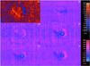 |
Fig. 4 a) Doppler shift (vlos) of Fe i 6302 derived with the bisector method. b) to f): differential line-of-sight velocities (as a comparison to 6302). b) 6302-6151. c) 6302-5250. d) 6302-5251. e) 6302-5248. f) 6302-6301. Top color scale refers to the a map. Bottom color scale refers to the b, f maps. The field-of-view is 160 × 110 arcsec2, observed on 17 August 1999 08:53 NOAA 8668. |
The Evershed flow (Evershed 1909) is a horizontal motion of photospheric gas. Many of spectroscopic observations have reported the vertical component of the flow in the penumbra (Johannesson 1993; Schlichenmaier & Schmidt 2000). Bellot Rubio et al. (2003) have demonstrated that the Evershed flow is aligned with the magnetic field in the penumbra of a sunspot, confirming that the field is frozen in the plasma.The inclination of the magnetic field has been found to be slightly higher than in the mean umbral background (Barthi et al. 2009). An outstanding puzzle about the Evershed flow is the relation between the velocity vector and the magnetic field vector in the penumbra. Because the averaged magnetic field vector in the penumbra has a significant vertical component, with an angle with respect to the normal vector on the solar surface between 40−80 degrees, and because the Evershed flow is apparently horizontal, this would mean that the flow moves across the magnetic field. Sánchez Almeida & Lites (1992) have already presented Stokes profile asymmetry observations from the part of the penumbra closest to the disk center (center side) in a sunspot that shows a smaller amplitude in the blue than in the red component. Müller et al. (2006) compared the net circular polarization maps to observations to show that a radial dependence on the limb-side is clearly reproduced.
We observed a vertical gradient of the horizontal component of the Evershed flow that would be compatible with a velocity vector parallel to the magnetic field. Figure 3 shows the distinct distribution of positive and negative gradients depending on the difference in the formation heights of these lines.
3.2. Differential Doppler shift
We investigate the self-consistency of the measurements obtained from inversion and bisector methods presented in Appendix C. We first defined the differential Doppler shift as the difference of the Doppler shift between two different lines derived from the quantitative bisector method. Figure 4 displays the differential line-of-sight velocity maps, i.e., the difference of the Doppler shift with respect to the Fe i 6302 Å line. The self-consistency of the modeling appears when comparing the gradient maps (derived from the inversion method) to the differential Doppler shift maps (obtained from the bisector method). Particularly, the measured differential map of the line-of-sight velocity (6301 minus 6302) from Doppler shift is highly correlated with the gradient map derived from the inversion. The patterns presented by the differential velocity and by the gradient maps show an opposite sign distribution between the disk center-side and the limb-side penumbra (Figs. 3 and 4). This result is consistent with the idea that a vertical component in the velocity vector in the penumbra is superposed to the Evershed flow, which is mainly horizontal. The Doppler shift distribution (vlos) of other lines (not represented in Fig. 4) is very similar to the velocities. The small bright blue patches in the umbra, especially for Fe i 5250.65 Å and Cr i 5247.57 Å, are caused by molecular lines that lead to wrong derivations from the measured profiles. There is almost no difference between the Doppler shifts, except when one derives the differential.
We followed the active region AR 8668 from 15 to 20 August to observe the evolution of the asymmetric distribution between the disk center-side and limb-side penumbra. We observed no twist or azimuthal rotation along the line-of-sight with respect to the sunspot center but only a geometrical projection of the line-of-sight direction along the AR motion on the solar disk.
 |
Fig. 5 Differential Doppler shift (vlos) of Fe i
6302−Fe i 6301 of the active region observed from 15 to 20 August 1999.
No twist or azimuthal rotation along the line-of-sight with respect to the sunspot
center is observed. The field-of-view is 160 × 110 arcsec2. The AR
coordinates are (15th (E 797 |
3.3. Vertical gradient of the magnetic field
In the following, we focus on selected points with a longitudinal magnetic field between 200 and 1000 Gauss, selected on the Fe i 6302.50 Å line map, and related to points lying in the network and the penumbra. Figure 6 depicts these regions. The network patches and the penumbra correspond to values of the magnetic field where a linear behavior correlation is determined between the magnetic field of the different lines. Moreover, we assumed a monotone strength decrease with height and considered the result of inverting each spectral line separately. Results from the different lines indicated in Fig. 7 yield the height dependence of the magnetic field. Balthasar & Gömöry (2008) have presented small features with a strong magnetic field that would expand rapidly with height. The canopy effect would be a possible explanation for magnetic fields that increase with height, as were also found by Socas-Navarro (2011). Most investigations find a decrease of the magnetic field strength with height (Orozco Suárez et al. 2005; Jurcàk et al. 2006). The magnetic field height gradient is mostly negative in the quiet Sun. As indicated by Fig. 7, except for the Cr i 5247.57 Å, we found an ordering similar to what was determined from the modeling of the formation heights in atmospheres of very bright network elements described in Appendix A (Vernazza et al. 1981).
Figure 9 shows the scatter plots obtained from a comparison with the Fe i 6302.50 Å line. Mean values of the longitudinal magnetic field of the lines of interest were calculated for intervals of 100 G of the corresponding longitudinal magnetic field of the Fe i 6302.50 Å line. The correlation breaks down for the weaker field for the longitudinal field below ~200 G. Below this limit our diagnosis is probably not sufficiently robust. If the field decreases with height, the Fe i line at 6151.6 Å is the lowest-formed one.
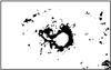 |
Fig. 6 Region delimited (in black) by magnetic field values from 200 to 1000 G on the map of the line Fe i 6302.50 Å. The field of view is 160 × 110 arcsec2. |
 |
Fig. 7 Mean longitudinal field strengths determined from inverting the different lines (abscissa). A regular decrease of the longitudinal magnetic field is found when ordering the following ions: Fe i 6151.62 Å, Fe i 5250.22 Å, Fe i 6302.50 Å, Cr i 5247.57 Å, Fe i 5250.65, and Fe i 6301.5 Å. The average is taken on a region delimited by magnetic field values from 200 to 1000 G on the map of the line Fe i 6302.50 Å, as indicated in Fig. 6. |
 |
Fig. 8 Formation heights (derived from the VAL F model) versus the mean longitudinal field strengths determined from inverting the different lines. A regular monotone decrease of the longitudinal magnetic field is found, corresponding to the ordering of the ions as indicated in Table 1. A vertical component gradient (absolute value) of the magnetic field of − 1.18 G/km is determined from the linear relationship. The average is taken on a region delimited by magnetic field values from 200 to 1000 G on the map of the line Fe i 6302.50 Å, as indicated in Fig. 6. Standard errors for the regression coefficients are 179.3 and 0.25 for the linear fit 1043.85 and − 1.11. |
The Fe i 5250.22 Å, and Fe i 6302.50 Å lines were observed simultaneoulsy by Socas-Navarro et al. (2008) to find a reliable indicator for the intrinsic field strength. In agreement with Socas-Navarro et al. (2008), we found that the 5250 and 6302 inversions are relatively similar. Nevertheless, we found that for points of medium magnetic field strength (200 to 1200 Gauss), the Fe i 6302.50 Å line is formed higher than the 5250.22 Å line, in agreement with the modeling of the formation heights in atmospheres of the quiet Sun and spot umbra (Appendix A). If the field strength decreases with height, one would expect to retrieve a slightly lower field strength for Fe i 6302.50 Å. Nevertheless, in the top scatter plot of Fig. 9, corresponding to the comparison between Fe i 6302.50 Å and 5250.22 Å, the points do not lie systematically above the diagonal of the plot, especially for points with a magnetic field exceeding 1200 G. In that case, the Fe i 5250.22 Å line is formed higher than 6302.50 Å one.
 |
Fig. 9 Scatter plots of the mean value of the longitudinal magnetic field of the different lines (ordinates) calculated for intervals of 100 G of the longitudinal field of Fe i 6302.50 Å (abscissa). Top to bottom left in ordinates: Fe i 5250.22 Å, Cr i 5247.57 Å, Fe i 5250.65 Å. Top to bottom right in ordinates: Fe i 6301.5 Å, and Fe i 6151.62 Å. A linear regime is determined for magnetic field values laying from 200 to 1200 G. |
All green lines, i.e., Fe i 5250.22 Å, Cr i 5247.57 Å, and Fe i 5250.65 Å, show a peculiar regime for strong fields related to bright and dark penumbral filaments, as indicated in Fig. 9. This behavior is likely related with their low-excitation potential. The lines become stronger and therefore come from higher layers in cool dark stuctures.
From modeling the line formation heights, we determined a vertical component gradient (absolute value) of the magnetic field of − 1.18 G/km as indicated in Fig. 8. By comparison, with the Tenerife Infrared Polarimeter (TIP) mounted on the VTT, Balthasar (2006) observed three Fe i lines at 15 648, 15 452, and 10 896 Å in eight spots. The spots were not all close to disk center, but the results were corrected for 3D effects. Balthasar applied the SIR inversion (Ruiz Cobo & del Toro Iniesta 1992) and determined the horizontal derivatives of the magnetic field and derived from them the vertical derivative (via div B = 0). He obtained a value of 0.5 G/km in the umbra. Measurements of the full Stokes vector were obtained with the two different spectral lines Fe i 10783 and Si i 10786 Å observed simultaneously by Balthasar & Gömöry (2008). These authors also applied the difference method, which yielded a different result. They found penumbral values varying between 1−2 G/km (Balthasar & Gömöry 2008). Westendorp Plaza et al. (2001) used the SIR inversion code to invert spectropolarimetric data of the same Fe i 6301.5 and 6302.5 Å photospheric lines observed with the Advanced Stokes Polarimeter. The SIR inversion code computed the line response functions so that the line formation depth was also derived. Westendorp Plaza et al. (2001) reported 1.5−2 G/km. With the Gregory-Coudé Telescope (GCT) at Tenerife, Pahlke & Wiehr (1990) observed the circular polarization of six lines in a spot umbra, Si i 6142.9 Å, Zr i 6143.2 Å, Fe ii 6149.2 Å, Ti i 6149.7 Å, Fe i 6151.6 Å, and Na i 6154.2 Å. These authors used a refined model of the circular polarization, which was applied with a magnetic field vertical gradient, and the best agreement between the six lines was a gradient of 2 G/km.
Formation heights in the model atmosphere of a very bright network element for the spectral lines of interest in the paper of the VAL F model.
4. Conclusion
We proposed an extension of the Unno-Rachkovsky solution assuming that asymmetries in Stokes polarization spectral line profiles can be attributed to gradients in the velocity (and magnetic field) over the line-forming region. We found our results in agreement with the modeling of height formation (Vernazza et al. 1981) for field strengths of approximately 0.2 kG up to 1.2 kG.
We obtained results with the inversion method (Bommier et al. 2007) as well as the quantitative bisector method (Rayrole 1967; Bommier et al. 2005) to show the self-consistency of the modeling. We applied the bisector method accurately for a stronger field, as has been intuited by Semel (1967). The first application would be to develop quick-look processing data codes able to operate during observations. A tomography of the 3D shape of the magnetic field depending on the formation height of the different lines of the solar atmosphere can then derived. Most observational studies of active-region magnetism are based on photospheric measurements that are used to infer the coronal field (Démoulin et al. 1997). To derive the magnitude and the time duration of the magnetic field, we propose to determine the free magnetic energy of the active region using maps of the vector magnetic field and inversion codes (Bommier et al. 2007; Molodij et al. 2011), and to measure the horizontal photospheric motions with local correlation tracking (Molodij et al. 2010) from high spatial resolution observations obtained from space- and ground-based observations using adaptive optics. A combination of vector magnetograms and Hα data would be of great interest to predict ejections of coronal mass in the interplanetary medium (Schmieder et al. 2011). Prospective projects are to study the evolution of the three components of the magnetic field in the corona and analyze the emerging flux derived from vector magnetograms where the azimuth ambiguity is solved in the photospheric vector magnetic field measurements from observations of 6301 and 6302 Å spectral lines.
Acknowledgments
We would like to thank the referees for the valuable remarks. Many thanks to Egidio Landi Degl’Innocenti for providing constructive comments. Special thanks to N. Globus for her wise advice. Based on observations made with the French-Italian telescope THEMIS operated by CNRS and CNR on the island of Tenerife in the Spanish Observatorio del Teide of the Instituto de Astrofísica de Canarias.
References
- Allende Prieto, C., & Garcia López, R. J. 1998, A&AS, 131, 431 [NASA ADS] [CrossRef] [EDP Sciences] [Google Scholar]
- Arnaud, J., & Faurobert, M. 2003, A&A, 412, 555 [NASA ADS] [CrossRef] [EDP Sciences] [Google Scholar]
- Asplund, M., Nordlund, A., Trampedach, R., Prieto, C. A., & Stein, R. F. 2000, A&A, 359, 729 [NASA ADS] [Google Scholar]
- Auer, L. H., & Heasley, J. N. 1978, A&A, 64, 67 [NASA ADS] [Google Scholar]
- Auer, L. H., Heasley, J. N., & House, L. L. 1977, Sol. Phys., 55, 44 [Google Scholar]
- Balasubramaniam, K. S., Keil, S. L., & Tomczyk, S. 1997, ApJ, 482, 1065 [NASA ADS] [CrossRef] [Google Scholar]
- Balthasar, H. 2006, A&A, 449, 1169 [NASA ADS] [CrossRef] [EDP Sciences] [Google Scholar]
- Balthasar, H., & Gömöry, P. 2008, A&A, 488, 1085 [NASA ADS] [CrossRef] [EDP Sciences] [Google Scholar]
- Balthasar, H., & Demidov, M. L. 2012, Sol. Phys., 280, 355 [NASA ADS] [CrossRef] [Google Scholar]
- Barthi, L., Joshi, C., Jaaffrey, S. N. A., & Jain, R. 2009, MNRAS, 393, 65 [NASA ADS] [CrossRef] [Google Scholar]
- Beckers, J. M. 1971, IAU Symp. 43 (Paris Reidel Publishing Co), 3 [Google Scholar]
- Beckers, J. M., & Schröter, E. H. 1969, Sol. Phys., 10, 384 [NASA ADS] [CrossRef] [Google Scholar]
- Bellot Rubio, L. R., Balthasar, H., Collados, M., & Schlichenmaier, R. 2003, A&A, 403, 47 [Google Scholar]
- Bommier, V. 2011, A&A, 530, A51 [NASA ADS] [CrossRef] [EDP Sciences] [Google Scholar]
- Bommier, V., & Molodij, G. 2002, A&A, 381, 241 [NASA ADS] [CrossRef] [EDP Sciences] [Google Scholar]
- Bommier, V., & Rayrole, J. 2002, A&A, 381, 227 [NASA ADS] [CrossRef] [EDP Sciences] [Google Scholar]
- Bommier, V., Rayrole, J., & Eff-Darwich, A. 2005, A&A, 435, 1125 [Google Scholar]
- Bommier, V., Landi Degl’ Innocenti, E., Landolfi, M., & Molodij, G. 2007, A&A, 464, 323 [NASA ADS] [CrossRef] [EDP Sciences] [Google Scholar]
- Bommier, V., Martínez González, Bianda, M., et al. 2009, A&A, 506, 1415 [NASA ADS] [CrossRef] [EDP Sciences] [Google Scholar]
- Borrero, J. M., & Ichimoto, K. 2011, Liv. Rev. Sol. Phys., 8, 4 [Google Scholar]
- Borrero, J. M., Tomczyk, S., Kubo, M., et al. 2010, Sol. Phys., 273, 267 [Google Scholar]
- Bruls, J. H. M. J., Lites, B. W., & Murphy, G. A. 1991, Proc. Eleventh NSO/Sac. Peak Summer Workshop, Solar Polarimetry, 27−31 August 1990, ed. L. J. November, 444 [Google Scholar]
- Démoulin, P., Bagala, L. G., Mandrini, C. H., Hénoux, J. C., & Rovira, M. G. 1997, A&A, 325, 305 [NASA ADS] [Google Scholar]
- Dravins, D., & Nordlund, A. 1990, A&A, 228, 184 [NASA ADS] [Google Scholar]
- Evershed, J. 1909, MNRAS, 69, 454 [NASA ADS] [CrossRef] [Google Scholar]
- Grec, C., Aime, C., Faurobert, M., Ricort, G., & Paletou, F. 2007, A&A, 463, 1125 [NASA ADS] [CrossRef] [EDP Sciences] [Google Scholar]
- Grigorjev, V. M., & Katz, J. M. 1972, Sol. Phys., 22, 119 [NASA ADS] [CrossRef] [Google Scholar]
- Henson, G. D., & Kemp, J. C. 1984, Sol. Phys., 93, 289 [NASA ADS] [CrossRef] [Google Scholar]
- Illing, R. M. E., Landman, D. A., & Mickey, D. L. 1974, A&A, 37, 97 [NASA ADS] [Google Scholar]
- Johannesson, A. 1993, A&A, 273, 633 [NASA ADS] [Google Scholar]
- Jurcàk, J., Martínez PIllet, V., & Sobotka, M. 2006, A&A, 453, 1079 [NASA ADS] [CrossRef] [EDP Sciences] [Google Scholar]
- Khomenko, E., & Collados, M. 2007, ApJ, 659, 1726 [NASA ADS] [CrossRef] [Google Scholar]
- Khomenko, E. V., Shelyag, S., Solanki, S. K., & Vogler, A. 2005, A&A, 442, 1059 [NASA ADS] [CrossRef] [EDP Sciences] [Google Scholar]
- Landi Degl’Innocenti, E., 1976, A&AS, 25 379 [NASA ADS] [Google Scholar]
- Landi Degl’ Innocenti, E., & Landolfi, M. 1982, Sol. Phys., 87, 221 [Google Scholar]
- Landman, D. A., & Finn, G. D. 1979, Sol. Phys., 63, 221 [NASA ADS] [Google Scholar]
- Landolfi, M., & Landi Degl’ Innocenti, E. 1982, Sol. Phys., 78, 355 [NASA ADS] [CrossRef] [Google Scholar]
- Landolfi, M., & Landi Degl’ Innocenti, E. 1996, Sol. Phys., 164, 191 [NASA ADS] [CrossRef] [Google Scholar]
- Landolfi, M., Landi Degl’ Innocenti, E., & Arena, P. 1984, Sol. Phys., 93, 269 [NASA ADS] [CrossRef] [Google Scholar]
- Lites, B. W., & Skumanich, A. 1990, ApJ, 348, 747 [NASA ADS] [CrossRef] [Google Scholar]
- Makita, M. 1980, in Proc. Japanese-France Seminar on Solar Physis, eds. F., Moriyama, & J. C. Hénoux, 99 [Google Scholar]
- Makita, M., & Ohki, Y. 1986, Ann. Tokyo Obs., 21, 1 [Google Scholar]
- Martínez PIllet, V. 2000, A&A, 453, 1079 [Google Scholar]
- Molodij, G., & Aulanier, G. 2012, Sol. Phys., 276, 451 [NASA ADS] [CrossRef] [Google Scholar]
- Molodij, G., & Rayrole, J. 2006, Solar Polarization 4, 19−23 Sept., 2005, Boulder, Colorado, eds. R. Casini, & B. W. Lites, ASP Conf. Ser., 358, 132 [Google Scholar]
- Molodij, G., Rayrole, J., Madec, P. Y., & Colson, F. 1994, A&AS, 118, 169 [NASA ADS] [CrossRef] [EDP Sciences] [Google Scholar]
- Molodij, G., Keil, S., Roudier, T., Meunier, N., & Rondi, S. 2010, JOSA.A, 27, 11, 2451 [CrossRef] [Google Scholar]
- Molodij, G., Bommier, V., & Rayrole, J. 2011, A&A, 531, A139 [NASA ADS] [CrossRef] [EDP Sciences] [Google Scholar]
- Moore, C. E. 1945, Contributions from the Princeton University Observatory, 20, 1 [Google Scholar]
- Müller, D. A. N., Schlichenmaier, R., Fritz, G., & Beck, C. 2006, A&A, 460, 925 [NASA ADS] [CrossRef] [EDP Sciences] [Google Scholar]
- Orozco Suárez, D., Lagg, A., & Solanki, S. K. 2005, in Chromospheric and Coronal Magnetic Fields, eds. D. E. Innes, A. Lagg, & S. K. Solanki (Germany: Katlenburg-Lindau), ESA SP, 596, 59 [Google Scholar]
- Orozco Suárez, D., Bellot Rubio, L. R., del Toro Iniesta, J. C., et al. 2007, ApJ, 670, 61 [Google Scholar]
- Pahlke, K.-D., & Wiehr, E. 1990, A&A, 228, 246 [Google Scholar]
- Paletou, F., Lopez Ariste, A., Bommier, V., & Semel, M. 2001, A&A, 375, 39 [Google Scholar]
- Rachkovsky, D. N. 1962, Izv. Crim. Astrphys. Obs., 25, 277 [Google Scholar]
- Rachkovsky, D. N. 1967, Izv. Crim. Astrphys. Obs., 37, 56 [Google Scholar]
- Rayrole, J. 1967, Ann. Astrophys., 30, 257 [NASA ADS] [Google Scholar]
- Rayrole J. 1971, IAU Symp. 43 (Paris: Reidel Publishing Co), 181 [Google Scholar]
- Ribes, E., Rees, D. E., & Fang, C. 1985, ApJ, 296, 268 [NASA ADS] [CrossRef] [Google Scholar]
- Roddier, C., & Roddier, F. 1993, Appl. Opt., 32, 16 [CrossRef] [Google Scholar]
- Ruiz Cobo, B., & del Toro Iniesta, J. C. 1992, ApJ, 398, 375 [NASA ADS] [CrossRef] [Google Scholar]
- Sánchez Almeida, J., & Lites, B. 1992, A&A, 398, 359 [Google Scholar]
- Schlichenmaier, R., & Schmidt, W., 2000, 358, 1122 [Google Scholar]
- Schmieder, B., Démoulin, P., Pariat, E., et al. 2011, Adv. Space Res., 47, 2081 [NASA ADS] [CrossRef] [Google Scholar]
- Semel, M. 1967, Ann. Astrophysique, 30, 513 [Google Scholar]
- Seykora, E. J. 1993, Sol. Phys., 145, 389 [NASA ADS] [CrossRef] [Google Scholar]
- Skumanich, A., & Lites, B. W. 1987, ApJ, 322, 473 [Google Scholar]
- Socas Navarro, H. 2011, A&A, 529, A37 [NASA ADS] [CrossRef] [EDP Sciences] [Google Scholar]
- Socas-Navarro, H., Borrero, J. M., Asensio Ramos, A., et al. 2008, ApJ, 674, 606 [Google Scholar]
- Solanki, S. K. 1985, A&A, 148, 123 [NASA ADS] [Google Scholar]
- Solanki, S. K., & Stenflo, J. O. 1984, A&A, 140, 185 [NASA ADS] [Google Scholar]
- Stenflo, J. O. 1971, IAU Symp. 43 (Paris Reidel Publishing Co), 101 [Google Scholar]
- Stenflo, J. O. 1973, Sol. Phys., 32, 41 [NASA ADS] [CrossRef] [Google Scholar]
- Stenflo, J. O., & Keller, C. U. 1996, Nature, 382, 588 [NASA ADS] [CrossRef] [Google Scholar]
- Stenflo, J. O., & Keller, C. U. 1997, A&A, 321, 927 [NASA ADS] [Google Scholar]
- Stenflo, J. O., Harvey, J. W., Brault, J. W., & Solanki, S. K. 1984, A&A, 131, 133 [NASA ADS] [Google Scholar]
- Trujillo Bueno, J., Collados, M., Paletou, F., & Molodij G. 2001, ASP Conf. Ser. 236, 11−15 Sept. 2000, ed. Sigmarth [Google Scholar]
- Uitenbroek, H. 2003, ApJ, 592, 1225 [NASA ADS] [CrossRef] [Google Scholar]
- Unno, W. 1956, Publ. Astr. Soc. Japan, 8, 108 [Google Scholar]
- Vernazza, J. E., Avrett, E. H., & Loeser, R. 1981, ApJS, 45, 635 [NASA ADS] [CrossRef] [Google Scholar]
- Westendorp Plaza, C., del Toro Iniesta, J. C., Ruiz Cobo, B., et al. 2001, ApJ, 547, 1130 [NASA ADS] [CrossRef] [Google Scholar]
- Wiese, W. L., 2012, http://www.nist.gov/pml/data/asd.cfm [Google Scholar]
- Wittmann, A. 1974, Sol. Phys., 35, 11 [NASA ADS] [CrossRef] [EDP Sciences] [Google Scholar]
Appendix A: Formation height models
Table 1 lists the formation heights in model atmospheres of very bright network elements for the spectral lines of interest from the VAL F model (Vernazza et al. 1981). To compute the line formation depth, we used the temperature, electron pressure and gas pressure from the atmospheric model. The continuum absorption coefficient was evaluated as in the MALIP code of (Landi Degl’Innocenti 1976), i.e., by including H− bound-free, H− free-free, neutral hydrogen atom opacity, Rayleigh scattering on H atoms, and Thompson scattering on free electrons. The line absorption coefficient was derived from the Boltzmann and Saha equilibrium laws, taking the first two ions of iron into account. The atomic data were taken from Wiese (2012) or Moore (1945) and the partition functions from Wittmann (1974). The iron abundance was assumed to be 7.60, and the chromium abundance 5.67 (in the usual logarithmic scale where the hydrogen abundance is 12). A depth-independent microturbulent velocity field of 1 km s-1 was introduced. Finally, for layers above τ5000 = 0.1, departures from LTE in the ionization equilibrium were simulated by applying Saha’s law with a constant “radiation temperature” of 5100 K instead of the electron temperature provided by the atmospheric model. To obtain the result, the line center optical depth grid was scaled to the continuum using the respective absorption coefficients. The continuum optical depth grid was the one provided with the atmospheric model and the transfer equation was not explicitly solved again. The formation height of the line center was then determined as follows. Given the grid of line center optical depths, the formation height of the line center is the height for which the optical depth along the line of sight is unity (Eddington-Barbier approximation), i.e., the height for which τ/μ = 1, where τ is the line center optical depth along the vertical, and μ the cosine of the heliocentric angle θ (here assumed to be 0). As can be seen in Fig. 5 of Bruls et al. (1991), this conveniently represents the depth where the contribution function has its maximum.
Appendix B: Observational setup
Spectroscopic performances and spatial resolution for three magnifying factors of the last transfer optics.
To obtain realistic measurements of the magnetic field simultaneously with determining the thermal and dynamic state of the solar atmosphere, we observed one region of the Sun simultaneously at different wavelength, as suggested by Rayrole (1967; 1971). To do this, Rayrole designed a telescope able to measure the physical parameters of the solar atmosphere quantitatively. During the campaign, we observed six different spectral lines indicated in Table B.2, i.e., a total of seven detectors (including the slit-field camera at 460.7 nm) were running perfectly synchronized. Table B.1 gives the spectral pixel, the spatial pixel, and the corresponding field of view for three magnifying factors of the optical setup. The instrumental configuration during the 1999 THEMIS campaign telescope has previously been described in detail (Molodij et al. 1996).
Appendix B.1: Polarimeter
The polarimeter is located at the telescope prime focus, before any oblique reflection in the optical path, and makes THEMIS a “polarization-free” telescope. The quarter wave plates are achromatic over a 400−700 nm spectral range; hence the phase of each of the plate is 90 ± 4deg in this range. In the 1999 instrumental setting configuration, the plates can be independently oriented at three different discrete angular positions across a 45 deg range of steps of 22.5deg. Depending on the quarter-wave plates orientation, the three Stokes parameter combinations are obtained successively. The entire scan of the region (160 × 110 arcsec2) took 35 min for ten spectral domains and the Stokes sequence (Q,U,V). Studies have previously been published to analyze the noise polarimetric sensitivity level for the non-magnetic FeI 5576 Å line (Bommier & Rayrole 2002). Since first light in 1998, interesting measurements such as quiet-Sun center-to-limb variations of the scattering polarization have been carried out, eventually modified by the Hanle effect (Stenflo & Keller 1996; Stenflo 1997). Typically, weak polarization was obtained at the limb with a sensitivity of Q/I ≃ 10-4 related to the so-called second solar spectrum (Trujillo-Bueno et al. 2001; Bommier & Molodij 2002; Arnaud & Faurobert 2003). The large photon collector and the high quality of the optical surfaces in combination with unique full-Stokes spectropolarimetry multiline capability improved our knowledge of the prominences in the magnetic field as indicated in Paletou et al. (2001).
Atomic parameters of lines observed during the 1999 campaign.
Appendix B.2: Spectral resolution
The two dispersers were used in additive mode (i.e., adding the grating dispersions) operating in its spectropolarimetric MTR (MultTi-Raies) mode. With the adapted slit masks in the predisperser focus plane (SP1) one can simultaneously select a number of spectral lines. The size of the spectral pixel, of the spatial pixel, and the observed field are defined when selecting the dispersion orders of the predisperser and the echelle spectrograph, and the magnification of the last transfer optics before the detectors. Three different gratings can be exchanged in the spectrograph when selecting the first disperser. Two of them (150 grooves/mm and 1200 grooves/mm) are commonly used for spectropolarimetry observations. The second spectrograph is a large camera mirror echelle grating (79 grooves/mm) that produces high dispersion-spectra of the domains selected by the masks in the focus plane (SP1). Table B.1 lists the spectral pixel, the spatial pixel, and the corresponding field-of-view after the last transfer optics when using the 150 grooves spectrograph with 384 pixels along the wavelength dispersion. The spectral resolution of the entire spectrograph and detector system was verified during this observational campaign. The system delivers a dispersion depending on the wavelength for the selected magnifying factor of the optics.
Appendix B.3: Spatial resolution
A testing method based on wavefront-curvature sensing (Roddier & Roddier 1993) has been applied to determine the permanent aberrations of the telescope and the transfer optics (up to 80 optical surfaces). The analysis has shown a wavefront dominated by astigmatisms coming principally from the entrance window and mechanical constraints on the primary mirror M1 of the telescope. The highest spatial resolution values were estimated at 0.3 up to 0.4 arcsec (λ = 0.5 μm). In this MTR configuration, the telescope system delivers a pixel resolution of 0.39 arcsec on the detector, i.e., an image resolution of 0.8 arcsec (≅4.5 times its diffraction limit). These performances were compared with space observations (Molodij & Aulanier 2012) and were verified by night time observations of stellar images using a curvature-wavefront analysis, from determining the temperature contrast analyzed via the intensity difference between the granule center and the intergranular lane, i.e., when determining statistically the root mean square of the intensity fluctuations expressed in units of the mean intensity of the granulation images at 4307 Å, and with a calibrated scintillometer (Seykora 1993).
Appendix B.4: Instrumental setup
The basic configuration of the MTR mode originally included twenty Thomson TH 7863 CMOS cameras (288 × 384 pixels 23 μm size), which were necessary to simultaneously record ten spectral domains in two Stokes parameters along 384 points. The high-speed data acquisition system can record one full CCD image per second and per camera. It is also possible to record subrasters of the field of view. The analogical digital converters are 12 bit-coded and cooled by Peltier cells refreshed by water circulation. The frame-reading time is about 236 ms and the acquisition-time setting from 2 ms up to 20 s. The frame-readings of all cameras are simultaneous while the digital conversion is sequential, so that the highest acquisition rate of the whole data acquisition system can record up to 14 acquisitions per second at the same time (3.1 Mo per second). In spite of a large full-well (106 charges), we report a limitation by the shot noise in the spot umbra for the exposure time (around 300 ms). The polarimetric resolution of 2 × 10⁻³ is currently achieved in one record on one pixel whose optimal size is set at 0.4 arcsec, the spectral resolution being lower than of 20 mÅ for the entire accessible spectral domain.
Appendix C: Quantitative bisector method
The different methods based on the Zeeman effect to measure the solar magnetic field have
been described and discussed by Beckers (1971). The
Zeeman effect refers to the splitting of spectral lines in the presence of a magnetic
field. This splitting is proportional to the field strength. The splitting pattern depends
on the atomic transition and on the magnetic field strength. The intensity of the Zeeman
components depends on the direction of the magnetic field. For strong fields and favorable
lines, the splitting is large enough to be directly measurable. In that case, it is rather
simple to measure both the strength and direction of the magnetic field (Rayrole 1967; Beckers 1969). But in solar physics, the Zeeman splitting
ΔλB is usually much smaller than the line
width. However, in that case, the splitting manifests itself through a polarization
variation along the line profile. This relation has been discussed in detail by Stenflo
(1971). The method used to measure all
interesting physical parameters requires determining a relative
displacement as precisely as possible. We used the method described in detail by
Bommier & Rayrole (2002) that was developed
by Rayrole (1967), in which the parameter to be
determined is not the line minimum (whose precise determination in discrete data may be
difficult), nor the line center of gravity, but the line bisector position at a given
depth in the profile (this depth is determined by the parameter
ng introduced below). A profile is given, for instance, by a
row of pixels of the image. To reduce the noise in the data that could disturb the
subsequent analysis, the first step is to perform a convolution of this data vector with a
normalized stepwise function of width ns pixels
 (C.1)The
width of the stepwise function ns is called the “slit width”
(as if the signal was entering a theoretical slit of width
ns). The result of the convolution is a smoothed profile
p(i). The second step is to derive the differences
between the convolved function values p(i) taken at
pixels separated by a quantity ng, which we
call the “slit gap” (as if two theoretical slits were placed at positions
i and i + ng). We compute
(C.1)The
width of the stepwise function ns is called the “slit width”
(as if the signal was entering a theoretical slit of width
ns). The result of the convolution is a smoothed profile
p(i). The second step is to derive the differences
between the convolved function values p(i) taken at
pixels separated by a quantity ng, which we
call the “slit gap” (as if two theoretical slits were placed at positions
i and i + ng). We compute
 (C.2)The abscissa of
the zero value of this last d(i) function is then
searched for, in terms of fractional pixels. A linear interpolation between two pixels
where d(i) takes values with opposite signs is
performed. Since the zero of d(i) falls near an
inflexion point of d(i), the linear interpolation is
accurate to the second order. The (generally fractional) i-value thus
obtained is taken as the line position. This method is very sensitive, reliable, and
precise as demonstrated in Bommier & Rayrole (2002).
(C.2)The abscissa of
the zero value of this last d(i) function is then
searched for, in terms of fractional pixels. A linear interpolation between two pixels
where d(i) takes values with opposite signs is
performed. Since the zero of d(i) falls near an
inflexion point of d(i), the linear interpolation is
accurate to the second order. The (generally fractional) i-value thus
obtained is taken as the line position. This method is very sensitive, reliable, and
precise as demonstrated in Bommier & Rayrole (2002).
Behaviors of magnetic and dynamic structures of the solar atmosphere are derived from the bisector method, which measures the shift of the two polarized spectral lines. Mass motions shift the two polarized spectral lines I + V and I − V in the same direction, whereas the magnetic field shifts the two lines in opposite spectral direction. The subtraction and the addition of the two opposite polarized spectra positions are related, to the line-of-sight magnetic field and the line-of-sight velocity respectively.
The longitudinal magnetic field component is determined from the difference between line positions determined with the bisector method in I + V and I − V spectra, denoted as Δλ (+ or −).
From the Zeeman effect law, associated to geometrical consideration, it can be shown that
(Semel 1967)
 (C.3)where
Δλ is expressed in mÅ, the wavelength λ in
μm. B is the field strength in Gauss,
ψ the angle between the magnetic field vector and the line-of-sight.
(C.3)where
Δλ is expressed in mÅ, the wavelength λ in
μm. B is the field strength in Gauss,
ψ the angle between the magnetic field vector and the line-of-sight.
 is the effective Landé factor given, for instance, by Bommier et al. (2005)
  (C.4)where
 (C.5)and
![Mathematical equation: \appendix \setcounter{section}{3} \begin{equation} \left\{ \begin{array}{c} J_{\rm s} = [J_{\rm u}(J_{\rm u}+1) + J_{\rm l}(J_{\rm l} + 1)] \\ J_{\rm d} = [J_{\rm u}(J_{\rm u}+1) - J_{\rm l}(J_{\rm l} + 1)] , \end{array} \right.\vspace{-2mm} \end{equation}](/articles/aa/full_html/2013/04/aa20427-12/aa20427-12-eq83.png) (C.6)where
u and l denote the upper and lower levels
respectively, and g is the Landé factor of a level of total kinetic
momemtum J.
(C.6)where
u and l denote the upper and lower levels
respectively, and g is the Landé factor of a level of total kinetic
momemtum J.
It is important to remark that no weak field approximation was performed, so that the law remains valid even for strong fields (Semel 1967).
The analytic relation between the wavelength fluctuations Δλ and the
velocity field v is
 (C.7)where v
is expressed in m s-1.
(C.7)where v
is expressed in m s-1.
The zero offset mean velocity is determined from the large field of view of 2 arcmin, invoking the velocity uniformity on large field of view. Therefore, the relative measurement is not affected by the line shift due to solar or earth rotations.
Clearly, to determine the field strength, one needs to know the thermodynamic state associated with the magnetic field. Thermal properties appear in the calibration of magnetographs, and the polarization profiles of spectrally resolved Stokes measurements provide not only vector field information, but also thermal and dynamic information. The absorption coefficient maps characterize the local thermodynamic parameters in which the magnetic field appears as a perturbation. This peculiar behavior is visible when observing the line depression map of Fe i 5576 Å, which is insensitive to the Zeeman effect, but nonetheless displays spatial variations generated by the magnetic field, as shown in Molodij & Rayrole (2006). This behavior is a direct consequence of the coupling between the thermodynamic state and the magnetic field. For the center-of-gravity method, a suggestion would be to separate the magnetic structure from the thermodynamic structure by simultaneous observations of magnetically sensitive and insensitive lines.
Nevertheless, the bisector method yields line position shifts that agree with the theoretical values derived from the computed theoretical profiles with the Unno (1956) and Rachkovsky (1962) models. The center-of-gravity method appears to be reliable for measuring velocities in the lower half of these formation heights and for measuring field strengths across the whole range of heights, for fields up to intermediate strength (Uitenbroek 2003).
All Tables
Formation heights in the model atmosphere of a very bright network element for the spectral lines of interest in the paper of the VAL F model.
Spectroscopic performances and spatial resolution for three magnifying factors of the last transfer optics.
All Figures
|
Fig. 1 UNNOFIT2 inversion code applied for ions Fe i 6301.5 Å, Fe i 5250.65 Å, and Fe i 6151.62 Å, which are anomalous Zeeman triplet, and the UNNOFIT inversion code applied on ions Cr i 5247.57 Å, Fe i 5250.22 Å, and Fe i 6302.50 Å, which are the normal triplet on the sunspot observed on 17 August 1999 08:53 NOAA 8668 with THEMIS. The longitudinal magnetic field component αBz is displayed in color (Gauss). The field of view is 160 × 110 arcsec2. The long-slit spectrograph gives a spectrum per acquisition. The entire observation from THEMIS consists of several successive steps of slit-scanning along a direction perpendicular to it, and results in a two-dimensional spatial map (100 scaning steps of the 0.4 arcsec × 100 arcsec slit). The interspace between two steps is 0.8 arcsec and the exposure time per frame is 0.3 s. A scan of the region (160 × 110 arcsec2) took 35 minutes for the six spectral domains. |
| In the text | |
|
Fig. 2 Same field of view of interest (160 × 110 arcsec2) of NOAA 8668
observed in the continuum of Fe i 6301.5 Å using a bandwidth slit of 18 m Å
with THEMIS (left) and observed in Hα
with the Big Bear Solar Observatory (right) on 17 August 1999 17:49
UT. The AR coordinates are E 507 |
| In the text | |
|
Fig. 3 Velocity differences derived from Stokes inversion analysis with the UNNOFIT/UNNOFIT2 code applied on a sunspot observed 17 August 1999 08:53 NOAA 8668 with THEMIS for ions Fe i 6301.5 Å, Fe i 5250.65 Å, Fe i 6151.62 Å, Cr i 5247.57 Å, Fe i 5250.22 Å, and Fe i 6302.50 Å. The additional determination of the vertical velocity differences is displayed and expressed in km s-1. The measurement of the different velocities that correspond to different formation heights (see Appendix A) allows to determine the velocity gradient. The field of view is 160 × 110 arcsec2. |
| In the text | |
|
Fig. 4 a) Doppler shift (vlos) of Fe i 6302 derived with the bisector method. b) to f): differential line-of-sight velocities (as a comparison to 6302). b) 6302-6151. c) 6302-5250. d) 6302-5251. e) 6302-5248. f) 6302-6301. Top color scale refers to the a map. Bottom color scale refers to the b, f maps. The field-of-view is 160 × 110 arcsec2, observed on 17 August 1999 08:53 NOAA 8668. |
| In the text | |
|
Fig. 5 Differential Doppler shift (vlos) of Fe i
6302−Fe i 6301 of the active region observed from 15 to 20 August 1999.
No twist or azimuthal rotation along the line-of-sight with respect to the sunspot
center is observed. The field-of-view is 160 × 110 arcsec2. The AR
coordinates are (15th (E 797 |
| In the text | |
|
Fig. 6 Region delimited (in black) by magnetic field values from 200 to 1000 G on the map of the line Fe i 6302.50 Å. The field of view is 160 × 110 arcsec2. |
| In the text | |
|
Fig. 7 Mean longitudinal field strengths determined from inverting the different lines (abscissa). A regular decrease of the longitudinal magnetic field is found when ordering the following ions: Fe i 6151.62 Å, Fe i 5250.22 Å, Fe i 6302.50 Å, Cr i 5247.57 Å, Fe i 5250.65, and Fe i 6301.5 Å. The average is taken on a region delimited by magnetic field values from 200 to 1000 G on the map of the line Fe i 6302.50 Å, as indicated in Fig. 6. |
| In the text | |
|
Fig. 8 Formation heights (derived from the VAL F model) versus the mean longitudinal field strengths determined from inverting the different lines. A regular monotone decrease of the longitudinal magnetic field is found, corresponding to the ordering of the ions as indicated in Table 1. A vertical component gradient (absolute value) of the magnetic field of − 1.18 G/km is determined from the linear relationship. The average is taken on a region delimited by magnetic field values from 200 to 1000 G on the map of the line Fe i 6302.50 Å, as indicated in Fig. 6. Standard errors for the regression coefficients are 179.3 and 0.25 for the linear fit 1043.85 and − 1.11. |
| In the text | |
|
Fig. 9 Scatter plots of the mean value of the longitudinal magnetic field of the different lines (ordinates) calculated for intervals of 100 G of the longitudinal field of Fe i 6302.50 Å (abscissa). Top to bottom left in ordinates: Fe i 5250.22 Å, Cr i 5247.57 Å, Fe i 5250.65 Å. Top to bottom right in ordinates: Fe i 6301.5 Å, and Fe i 6151.62 Å. A linear regime is determined for magnetic field values laying from 200 to 1200 G. |
| In the text | |
Current usage metrics show cumulative count of Article Views (full-text article views including HTML views, PDF and ePub downloads, according to the available data) and Abstracts Views on Vision4Press platform.
Data correspond to usage on the plateform after 2015. The current usage metrics is available 48-96 hours after online publication and is updated daily on week days.
Initial download of the metrics may take a while.